Simulation of the quantum dynamics of indistinguishable bosons with the method of coupled coherent states

(1)

bosons with the method of coupled coherent states

.

White Rose Research Online URL for this paper:

http://eprints.whiterose.ac.uk/147211/

Version: Accepted Version

Article:

Green, JA orcid.org/0000-0002-5036-3104 and Shalashilin, DV

orcid.org/0000-0001-6104-1277 (2019) Simulation of the quantum dynamics of

indistinguishable bosons with the method of coupled coherent states. Physical Review A,

100 (1). 013607. ISSN 2469-9926

https://doi.org/10.1103/PhysRevA.100.013607

©2019 American Physical Society. This is an author produced version of an article

accepted for publication in Physical Review A. Uploaded in accordance with the publisher's

self-archiving policy.

eprints@whiterose.ac.uk https://eprints.whiterose.ac.uk/ Reuse

Items deposited in White Rose Research Online are protected by copyright, with all rights reserved unless indicated otherwise. They may be downloaded and/or printed for private study, or other acts as permitted by national copyright laws. The publisher or other rights holders may allow further reproduction and re-use of the full text version. This is indicated by the licence information on the White Rose Research Online record for the item.

Takedown

If you consider content in White Rose Research Online to be in breach of UK law, please notify us by

(2)

Coherent States Method

James A. Green1, 2,∗ _{and Dmitrii V. Shalashilin}1,†

1_{School of Chemistry, University of Leeds, Leeds LS2 9JT, United Kingdom} 2_{Consiglio Nazionale delle Ricerche, Istituto di Biostrutture e Bioimmagini (CNR-IBB),}

via Mezzocannone 16, 80136, Napoli, Italy (Current Address) (Dated: June 9, 2019)

Computer simulations of many-body quantum dynamics of indistinguishable particles is a chal-lenging task for computational physics. In this paper we demonstrate that the method of coupled coherent states (CCS) developed previously for multidimensional quantum dynamics of distinguish-able particles can be used to study indistinguishdistinguish-able bosons in the second quantisation formalism. To prove its validity, the technique termed here coupled coherent states for indistinguishable bosons (CCSB) is tested on two model problems. The first is a system-bath problem consisting of a tunnelling mode coupled to a harmonic bath, previously studied by CCS and other methods in distinguishable representation in 20 dimensions. The harmonic bath is comprised of identical oscil-lators, and may be second quantised for use with CCSB, so that this problem may be thought of as a bosonic bath with an impurity. The cross-correlation function for the dynamics of the system and Fourier transform spectrum compare extremely well with a benchmark calculation, which none of the prior methods of studying the problem achieved. The second model problem involves 100 bosons in a shifted harmonic trap. Breathing oscillations in the 1-body density are calculated and shown to compare favourably to a multiconfigurational time-dependent Hartree for bosons calcu-lation, demonstrating the applicability of the method as a new formally exact way to study the quantum dynamics of Bose-Einstein condensates.

I. INTRODUCTION

In the past two decades there has been significant inter-est in systems of indistinguishable bosons, due to exper-imentally produced Bose-Einstein condensates of ultra-cold alkali metal atoms [1–3]. These condensates, first posited by the eponymous Bose and Einstein in 1924-25, have permitted macroscopic observations of quan-tum phenomena and lead to a wealth of experimental re-search in areas such as atomic interferometry [4], bosonic Josephson junctions [5, 6], quantum vortices [7, 8] and the generation of solitons [9,10].

From the theoretician’s point of view, the Gross-Pitaevskii equation (GPE) [11, 12] has been the pre-dominant method used to study Bose-Einstein conden-sates, see for example Refs. [13–18] and the review ar-ticles [19, 20]. However the GPE is a mean-field the-ory and as such cannot describe many-body effects in condensates. It also assumes that all bosons occupy a single state at all times, which is not the case dur-ing fragmentation. In recent years, the multiconfigura-tional time-dependent Hartree method for bosons (MCT-DHB) [21, 22] has been used to treat indistinguishable bosons from the standpoint of exact quantum mechan-ics [23–33]. A multi-layer version of MCTDHB has also been developed (ML-MCTDHB) [34,35] that exploits the multi-layer structure to study mixed bosonic systems (for example impurities in Bose-Einstein condensates [36–40],

∗_{j.a.green1@leeds.ac.uk} †_{d.shalashilin@leeds.ac.uk}

binary mixtures of Bose-Einstein condensates [41], and solitons [40,42–44]) and bosonic systems where different degrees of freedom may be separated (for example differ-ent spatial locations when bosons are residing in optical lattices [45–52]).

Before being used to treat indistinguishable bosons, standard MCTDH [53] and ML-MCTDH [54, 55] have been well established theories for treating distinguish-able particles. They are distinguish-able to solve the time-dependent Schr¨odinger equation (TDSE) exactly for multiple de-grees of freedom, albeit with basis sets that grow expo-nentially with increased dimensionality. Our own coupled coherent states (CCS) method has also demonstrated its propensity at solving the TDSE for distinguishable par-ticles, with basis sets that scale more favourably with di-mensionality [56,57]. This is achieved by using randomly sampled trajectory guided coherent states as basis func-tions, although the trade-off for this favourable scaling is that random noise and slow convergence may be present. Noise can cause a decay in auto/cross-correlation func-tions and may be reduced by increasing the number of configurations, or applying a filter diagonalisation tech-nique to extract frequencies [58]. Importance sampling of coherent state basis set initial conditions is also key to the accuracy and efficiency of the CCS approach [59].

(3)

the basis in CCSB is guided by classical-like trajectories, suggest that the method will be particularly suited to such systems. Indeed, recent semiclassical coherent state work with the Herman-Kluk method on indistinguishable bosons demonstrates this hypothesis [60, 61]. CCSB is fully quantum however, as with standard CCS, and it has previously been shown that a local quadratic approxima-tion of the Hamiltonian into the CCS equaapproxima-tions yields the coherent state matrix of the Herman-Kluk propa-gator [62]. We anticipate that the CCSB method will provide a description of many-body dynamics over and above the mean-field Gross-Pitaevskii approach. Fur-thermore, as CCS has previously shown to be able to pro-vide a similar numerical picture to MCTDH with lower computational scaling with dimensionality [63], we antic-ipate that CCSB may be able to do the same with respect to MCTDHB.

To illustrate the suitability of CCSB to problems in-volving indistinguishable bosons, we apply the method to two model problems. The first model problem con-sists of a bosonic bath with an impurity, demonstrating that the method is capable of studying multi-component bosonic systems and opening up the possibility of study-ing multi-atomic Bose-Einstein condensates [64], spinor Bose-Einstein condensates [65], dark-bright solitons [66], and Bose-polarons [67]. The second model problem con-sists of a collection of indistinguishable bosons in a har-monic trap, demonstrating the propensity of the method to study systems of bosons in optical lattices [68], for example with the Bose-Hubbard model [60, 61,69], and the possibility to study bosons in a single well that is deformed into a double well, such as that in Ref. [22], and observed in experimental bosonic Josephson junc-tions [70,71].

II. NUMERICAL DETAILS

The CCSB method relies on the machinery of the CCS method, which has been derived and presented previously when treating distinguishable particles [56, 57]. A de-scription of the CCS method will be presented below, before a discussion on how the method is modified to treat indistinguishable bosons in the second quantisation representation in CCSB.

A. Coupled Coherent States Working Equations

In the CCS method, the wavefunction is represented as a basis set of trajectory guided coherent states,|zi. The coordinate representation of a coherent state is given by

hx|zi=γ

π

1/4

exp

−γ₂(x−q)2+ i

~p(x−q) +

ipq

2~

,

(1) where q and pare the position and momentum centres of the coherent state, γ is the width parameter of the

coherent state, given byγ=mω/~_{, with} _m_{mass and}_ω frequency. In atomic units (which are used throughout the paper)m=ω =~_{= 1, thus}_γ_{= 1. Coherent states} are eigenstates of the creation and annihilation operators respectively

hz|ˆa†=hz|z∗ (2a) ˆ

a|zi=z|zi, (2b)

where the creation and annihilation operators are given by

ˆ

a†= √1

2(ˆq−ipˆ) (3a)

ˆ

a= √1

2(ˆq+ipˆ). (3b) The eigenvalues of Eqs.2aand2b,z∗ _and_z_{, can be used} to label a coherent state, and from Eqs.3aand3bit can be seen they are given by

z∗=√1

2(q−ip) (4a)

z=√1

2(q+ip). (4b) An important consequence of the above is that one may write a Hamiltonian in terms of creation and annihila-tion operators rather than posiannihila-tion and momentum op-erators. A normal ordered Hamiltonian may then be ob-tained when the creation operators precede the annihila-tion ones

ˆ

H(ˆq,pˆ) = ˆH(â,â†) =Hord(â†,â). (5)

From this, matrix elements of the Hamiltonian are simple to calculate in a coherent state basis

hz′|Hord(ˆa†,aˆ)|zi=hz′|ziHord(z′∗, z), (6)

where the overlaphz′_|_z_i_{is given by}

hz′|zi= exp

z′∗z−z

′∗_z′

2 −

z∗_z 2

. (7)

The wavefunction ansatz in CCS is given by

|Ψ(t)i=

K

X

k=1

Dk(t)eiSk(t)|zk(t)i, (8)

where the sum is over K configurations, Dk is a time

dependent amplitude andSk is the classical action. The

classical action in coherent state notation is given by

Sk=

Z _i

2(z ∗

kz˙k−z˙k∗zk)−Hord(zk∗, zk)

dt. (9)

The wavefunction is propagated via the time-dependence of the coherent state basis vectors, amplitudes and ac-tion. The coherent states are guided by classical trajec-tories, and evolve according to Hamilton’s equation

˙

zk=−i

∂Hord(z∗k, zk)

∂z∗

k

(4)

The time-dependence of the amplitudes may be found via substitution of Eq.8into the time-dependent Schr¨odinger equation and closing with a coherent state basis bra:

K

X

l=1

hzk|zlieiSl

dDl

dt =−i

K

X

l=1

hzk|zlieiSlDlδ2Hord(zk∗, zl),

(11) where theδ2Hord′ (zk∗, zl) term is

δ2Hord′ (zk∗, zl) =Hord(z∗k, zl)−Hord(zl∗, zl)−iz˙l(z∗k−zl∗).

(12) Finally, the time-dependence of the classical action is straightforwardly calculated from Eq.9.

B. Second Quantisation and CCSB

CCS works for Hamiltonians that can be expressed via creation and annihilation operators in the normal ordered form as illustrated in Eq. 6. As in second quantisation the Hamiltonian of a system of bosons has exactly such form no modifications of the working equations are re-quired for treating indistinguishable bosons with CCSB. The only difference is that the coherent state basis func-tions are used to represent particle number occupafunc-tions of quantum states in the second quantisation formalism, as opposed to individual particles in the distinguishable first quantisation representation.

In the second quantisation representation, multiparti-cle states are described in terms of an occupation number

n(α) _{that describes the number of particles belonging to}

a particular quantum state |αi. A Fock state describes the set of occupation number states

|n_i=

Ω

Y

α=0

|n(α)_i₌_|_n(0)_{, n}(1)_{, . . . , n}(Ω)_i_, ₍₁₃₎

and may be generated by successive application of cre-ation operators on the vacuum state|0i

|n(0), n(1), . . . , n(Ω)i= ˆ

a(0)†n(0)

√ n(0)_!

ˆ

a(1)†n(1)

√

n(1)_! . . .

ˆ

a(Ω)†n(Ω)

√

n(Ω)_! |0

(0)_,₀(1)_{, . . . ,}₀(Ω)

i.

(14)

In CCSB, the multidimensional version of the CCS wave-function representation is used as a basis set expansion for Fock states

|n_i=

K

X

k=1

Dk(t)eiSk(t)|zk(t)i, (15)

which is exactly analogous to Eq.8. The only difference is the multidimensional coherent state|zkiis a product of

coherent states that describe occupations of each quan-tum state|αi

|zki= Ω

Y

α=0

|z(α)i. (16)

Therefore any wavefunction in the basis of Fock states can be equivalently represented in the basis of coherent states. The Hamiltonian of a system of indistinguishable bosons can be second quantised and presented in terms of 1-body ˆh(Q), 2-body ˆW(Q,Q′), and creation and an-nihilation operators as

ˆ

H =X

α,β

hα|ˆh|βiˆa(α)†_ˆ_a(β)

+1 2

X

α,β,γ,ζ

hα, β|Wˆ|γ, ζiˆa(α)†aˆ(β)†ˆa(ζ)aˆ(γ),

(17)

where|αi,|βi,|γi, and|ζiare quantum states. This con-veniently gives a second quantised Hamiltonian in normal ordered form, which is required by CCSB. In the follow-ing sections CCSB is applied to two model problems to illustrate its ability to study fully quantum bosonic prob-lems and compare to numerically exact results.

III. APPLICATION 1: DOUBLE WELL

TUNNELLING PROBLEM

The first application of CCSB is to an M-dimensional model Hamiltonian that consists of an (M − 1)-dimensional harmonic bath, coupled to a 1-1)-dimensional tunnelling mode governed by an asymmetric double well potential. This a system-bath problem, which may also be thought of as a bosonic bath with an impurity, previ-ously studied in distinguishable representation with lin-ear coupling of the bath to the system by matching pur-suit split-operator Fourier transform (MP/SOFT) [72], standard CCS [73], a trajectory guided configuration in-teraction (CI) expansion of the wavefunction [74], an adaptive trajectory guided (aTG) scheme [75], Gaus-sian process regression (GPR) [76], and a basis expan-sion leaping multi-configuration Gaussian (BEL MCG) method [77]. It has also been studied with quadratic coupling of the bath to the system by MP/SOFT [72], standard CCS [73], trajectory guided CI [74], aTG [75] and a 2-layer version of CCS (2L-CCS) [78]. A bench-mark calculation for the quadratic coupling case has also been proposed in recent work [79], using a relatively sim-ple wavefunction expansion in terms of particle in a box wavefunctions for the tunnelling mode, and harmonic os-cillator wavefunctions for the harmonic bath. The size of the calculation in Ref. [79] was greatly reduced by exploiting the indistinguishability of the bath configu-rations, the first time this had been considered, and a well converged result was achieved, prompting the idea of CCSB. The quadratic coupling case is the one we con-sider in this application.

The Hamiltonian is given in distinguishable represen-tation by

ˆ

H =pˆ

(1)2

2 −

ˆ

q(1)2

2 +

ˆ

q(1)4

16η +

ˆ P2

2 +

1 +λqˆ(1)_ˆ

Q2

(5)

where (ˆq(1)_,_p_ˆ(1)_{) are the position and momentum}

op-erators of the 1-dimensional system tunnelling mode, and ( ˆQ,P) are the position and momentum operatorsˆ of the (M −1)-dimensional harmonic bath modes, with

ˆ Q=PM

m=2qˆ(m)and ˆP=

PM

m=2pˆ(m). The coupling

be-tween system and bath is given by the constantλ, whilst

η determines the well depth.

In previous work [72–75, 78, 79], the parameters λ= 0.1 and η = 1.3544 have been used in a 20-dimensional (M = 20) problem, which we also consider. The ini-tial wavefunction|Ψ(0)iis a multidimensional Gaussian wavepacket, with initial position and momentum centres for the tunnelling mode ˆq(1)_{(0) =}₋₂_._{5 and ˆ}_p(1)_{(0) = 0}_._0,

and for the bath modes ˆq(m)_{(0) = 0}_._{0 and ˆ}_p(m)_{(0) = 0}_.₀

∀m.

As the bath oscillators have the same initial

condi-tions and the same frequency, they can be thought of as indistinguishable, and the bath part of the Hamilto-nian may be second quantised for use with CCSB. As the tunnelling mode is not part of this indistinguishable system, the portion of the Hamiltonian that describes it will not be second quantised. However, this will not pose a problem as the dynamical equations are identical for CCS and CCSB, the only subtlety is the interpreta-tion of the coherent state basis vectors|z_ias will be dis-cussed below. Using the definition of a second quantised Hamiltonian in Eq. 17, and the definition of coherent states as eigenstates of the creation and annihilation op-erators, Eq.18may be written in normal-ordered form as

Hord(ˆa†,aˆ), for which the coherent state matrix element

hzk|Hord(ˆa†,aˆ)|zli=hzk|zliHord(z∗k,zl), where

Hord(z∗k,zl) =−

1 2

z_k(m=1)∗2+z(m=1)_l 2+ 1 64η

z_k(m=1)∗4+z(m=1)_l 4+ 4z_k(m=1)∗3z_l(m=1)+ 4z_k(m=1)∗z(m=1)_l 3

+6z(m=1)k ∗2z (m=1)2

l + 12z (m=1)∗

k z

(m=1) l + 6z

(m=1)∗2

k + 6z (m=1)2

l + 3

+

Ω

X

α=0

zk(2α)∗z (2α) l ǫ(2α)+

λ

2

Ω

X

α,β=0

zk(2α)∗z (2β)

l Q(2α,2β)

2

zk(m=1)∗+z (m=1) l

.

(19)

The quantum states |αi and |βi in Eq. 19 are those of the harmonic oscillator withαandβ numbers of quanta,

ǫ(α) _{is the eigenvalue for}_|_α_i_{, and the position and}

mo-mentum operators of the tunnelling mode have explic-itly been labelled with (m = 1) to distinguish them from theαlabelling scheme of the second quantised bath modes. A full derivation of this, alongside evaluation of the Q(2α,2β)2 _{matrix element is shown in Appendix} _A_.

Note that only even harmonic oscillator levels are re-quired due to all bath modes initially residing in the ground level, as previously assumed [79], and the bath having quadratic coupling to the system meaning only even harmonic oscillator levels will be occupied.

The multidimensional coherent state basis vector|z_iis represented as

|z_i=|z(m=1)i ×

Ω

Y

α=0

|z(2α)i, (20)

where|z(m=1)_i_{is a basis function for the tunnelling mode}

and |z(2α)_i _{is a basis function for the second quantised}

bath modes. The determination of initial conditions for these coherent state basis functions, as well as the values of the initial amplitudes is shown in the following section.

A. Initial Conditions for Application 1

The initial coherent state basis functions for the tun-nelling mode are sampled from a Gaussian distribution

centered around the initial tunnelling mode coordinates and momenta, as in previous works [73,78]

f(z(m=1))∝exp

−σ(m=1) z

(m=1)

−z(m=1)(0)

2

,

(21) whereσ(m=1) _{is a parameter governing the width of the}

distribution.

Sampling the initial coherent states for the bath can be performed by obtaining a probability distribution from the square of the coherent state representation of the initial bath Fock state. The initial bath Fock state is equal to

|n_i=

Ω

Y

α=0

|n(2α)_i

=|n(2α=0)_{, n}(2α=2)_{, . . . , n}(2α=2Ω)_i

=|(M−1),0, . . . ,0i,

(22)

where there areM−1 bath oscillators all in the ground harmonic oscillator state. Using the representation of a coherent state in a basis of Fock states

|zi= e−|

z|2

2 X

n(α) zn(α)

p

n(α)_!)|n (α)

i (23)

the following may be obtained

| hz(2α)|n(2α)i |2= e −|z(2α)_|2

|z(2α)|2n(2 α)

(6)

where the value ofπhas appeared to enforce normalisa-tion. This resembles a Poissonian distribution, however

|z(2α)_|2 _{is continuous so a gamma distribution is used}

instead

f(|z(2α)|2)∝ |z

(2α)_|2n(2 α)

e−|

z(2α)|2 σ(2α)

Γ(n(2α)_{+ 1)} _σ(2α)n(2α)+1, (25)

where σ(2α) _{is a compression parameter controlling the}

width of the distribution, and Γ is the gamma function that is calculated usingn(2α)+ 1 because Γ(n) = (n−1)!. The gamma distribution will be centred around

σ(2α)_n(2α)_{, however} _{| h}_z(2α)_|_n(2α)_{i |}2 _{should be centred}

around|z(2α)_|2₌_n(2α)_{as its maximum is found by}

d| hz(2α)_|_n(2α)_{i |}2

d|z(2α)_|2 =

1

πn(2α)_!

−e−|z(2α)|2|z(2α)|2n (2α)

+n(2α)e−|z(2α)|2|z(2α)|2n (2α)

−1

= 0. (26)

Fortunately, this is not an issue, as when n(2α) _{= 0}

for states 2α > 0, the distribution will be centred around 0 irrespective of the compression parameter, and for n(2α=0)₌_M₋_{1 a compression parameter of}

σ(2α=0)_{= 1}_._{0 is used. As we are not constrained by a}

choice of compression parameter σ(2α>0) _{for the states}

2α > 0, we are free to alter it to influence the accuracy of the calculation, and the final result presented in the following section usesσ(2α>0)_{= 100. The affect of}

alter-ing this parameter is discussed in Sec.III C.

The initial amplitudes are calculated by projection of the initial basis onto the initial wavefunction with the action set to zero

hzk(0)|Ψ(0)i= K

X

l=1

Dl(0)hzk(0)|zl(0)i. (27)

The overlap of the initial coherent state basis with the initial wavefunction can be decomposed to

hzk(0)|Ψ(0)i=hz(m=1)k (0)|Ψ

(m=1)₍₀₎

i h

Ω

Y

α=0

z_k(2α)(0)|n)i.

(28) The coherent state overlap with initial tunnelling mode wavefunction hz_k(m=1)(0)|Ψ(m=1)₍₀₎_i _{can be calculated}

via a Gaussian overlap, Eq.7, using the initial positions and momenta for the tunnelling mode ˆq(m=1)_{(0) =}₋₂_.₅

and ˆp(m=1)_{(0) = 0}_._{0. The coherent state overlap with}

initial bath Fock state can be calculated by once more using the coherent state representation in a basis of Fock states, Eq.23

h

Ω

Y

α=0

z(2α)_k (0)|n)i=

" Ω

Y

α=0

e−|z

(2α)

k (0)|

2

#

(z(2α=0)_k ∗(0))M−1

p

(M−1)! . (29)

B. Results and Comparison to Other Methods

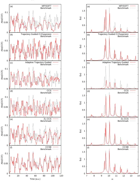
The quantity of interest used to assess the performance of CCSB and compare it to previous methods of study-ing the problem [72–75, 78, 79] is the cross-correlation function (CCF). This is the overlap between the wave-function at time t and the mirror image of the initial wavepacket, |Ψ(0)¯ i, i.e. hΨ(0)¯ |Ψ(t)i. The mirror im-age of the initial state has coordinates for the tunnelling mode of ¯q(1)(0) = +2.5 and ¯p(1)(0) = 0.0, with bath modes in the ground harmonic level. It is located in the upper well of the asymmetric double well tunnelling potential, therefore non-zero values of the CCF are in-dicative of tunnelling. The spectrum of the CCF is also presented via a Fourier transform (FT) of the real part of the CCF.

(7)

(i)

0 0.05 0.1

0 20 40 60 80 100 120 (f)

Abs(CCF)

Time (a.u.)

BenchmarkCCSB 0

0.05 0.1

(e)

Abs(CCF)

Benchmark 2L-CCS 0

0.05 0.1

(d)

Abs(CCF)

Benchmark CCS 0

0.05 0.1

(c)

Abs(CCF)

Benchmark Adaptive Trajectory Guided 0

0.05 0.1

(b)

Abs(CCF)

Benchmark Trajectory Guided CI Expansion 0

0.05 0.1

(a)

Abs(CCF)

Benchmark MP/SOFT

(ii)

0 0.5 1 1.5

7 8 9 10 11 12 13 14 (f)

I

(

ω

)

ω

BenchmarkCCSB 0

0.5 1 1.5

(e)

I

(

ω

)

Benchmark 2L-CCS 0

0.5 1 1.5

(d)

I

(

ω

)

Benchmark CCS 0

0.5 1 1.5

(c)

I

(

ω

)

Benchmark Adaptive Trajectory Guided 0

0.5 1 1.5

(b)

I

(

ω

)

Benchmark Trajectory Guided CI Expansion 0

0.5 1 1.5

(a)

I

(

ω

)

[image:7.612.81.529.70.647.2]

Benchmark MP/SOFT

FIG. 1: Comparison of (i) absolute values of the cross-correlation functions and (ii) Fourier transforms of the real part of the cross-correlation functions for different methods (red, solid) of studying Eq.18withM = 20. λ= 0.1

(8)

is achieved in CCSB by taking account of the symmetry of the Hamiltonian.

The CCSB calculation uses K = 4000 configurations and Ω = 5 even harmonic oscillator levels in the bath basis. The dimensionality of this problem has therefore been reduced from 20 to 6. The influence on the CCSB calculation of altering these parameters, as well as the compression parameter chosen ofσ(2α>0)_{= 100 is shown}

in the following section.

C. Numerical Accuracy and Convergence

Using an approach first presented in Ref. [78] to illus-trate the accuracy and convergence of a method studying Application 1 with respect to the benchmark calculation, we define an error parameterχas

χ=

Z

|Abs(hΨ(0)¯ |Ψ(t)i)bench

−Abs(hΨ(0)¯ |Ψ(t)i)CCSB|dt,

(30)

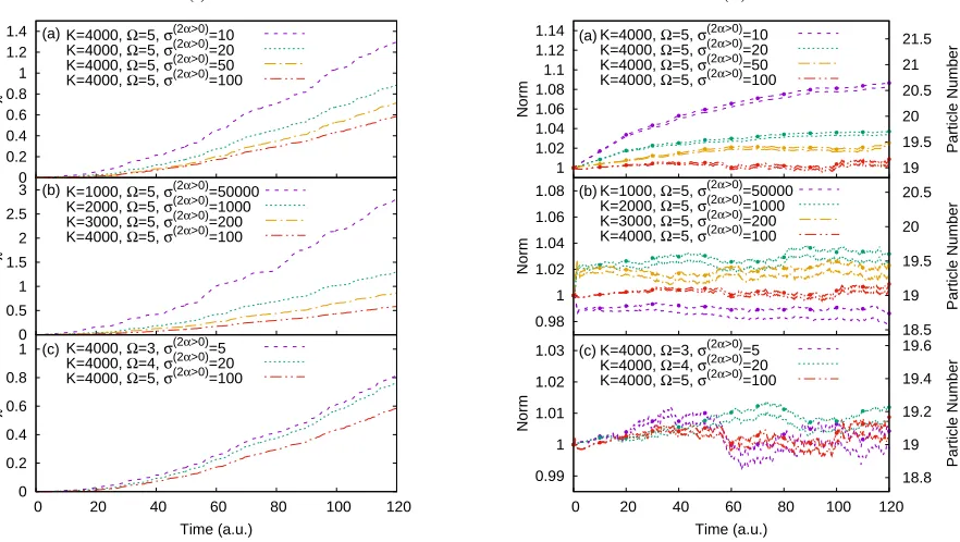
which indicates the cumulative error of the absolute value of the cross-correlation function of the CCSB method compared to the benchmark. This is shown in Fig.2(i) for different values of σ(2α>0)_, _K _{and Ω, in panels (a),}

(b) and (c).

As with CCS, the CCSB method does not conserve the normhΨ(t)|Ψ(t)iby default due to the use of a basis consisting of a superposition of coherent states [57]. How-ever, this can be a useful property as the extent of norm conservation can be used to determine the accuracy and reliability of a propagation. Another important quantity for CCSB to conserve is the total particle number

N=hΨ(t)|

Ω

X

α=0

ˆ

a(α)†ˆa(α)|Ψ(t)i

=

K

X

k,l=1 Ω

X

α=0

D∗

kDlei(Sl−Sk)hzk|zliz(α)k ∗z (β) l ,

(31)

which for Application 1 amounts to the number of os-cillators in the bath, N = (M −1) = 19. Plots of the norm and particle number conservation for different val-ues of σ(2α>0)_, _K_{, and Ω, (as in Fig.} _2(i)_{), are shown}

in Fig. 2(ii), with the value of the norm given by the dashed/dotted lines without circles and the particle num-ber by the dashed/dotted lines with circles. It can be seen that the values of the norm and particle number follow each other closely for all calculations, and we will discuss the specific cases in the following.

Firstly, considering panel (a) in Figs. 2(i) and 2(ii), both K and Ω are held fixed whilst σ(2α>0) _{is varied.}

It can be seen that the quality of the calculation with respect to the error term χ, and the conservation of the norm and particle number improves with increasing

σ(2α>0)_{. Further increase of}_σ(2α>0)_{results in a}

numeri-cally unstable propagation, as the value of the norm and

particle number explodes as the basis is overcompressed. This suggests that appropriate choice ofσ(2α>0) _is

nec-essary for the initial sampling of the coherent states, as a value that is too small leads to errors due to the co-herent states spreading too quickly, whilst a value that is too large leads to numerical instability.

Secondly, considering panel (b) in Figs. 2(i)and 2(ii), the value ofK is varied whilst Ω is held constant. The value of σ(2α>0) _{was chosen based on the criteria}

pre-sented in the previous paragraph, with larger values of

σ(2α>0) for smaller values of K. This phenomenon has been noted in previous studies with CCS, where larger compression parameters are necessary for basis sets with fewer configurations, see Ref. [59] for further details. The error χ decreases with increasing K, as Monte-Carlo noise causing decay of the cross-correlation function de-creases with increasing number of configurations. How-ever,χdoes not remain at 0 for the duration of the calcu-lation, and theK= 4000 propagation is only equivalent to theK= 3000 calculation for the first 30 a.u. This in-dicates the slow convergence of the method as mentioned in the introduction. However, we can regard the accuracy of theK= 4000 calculation as sufficient for this applica-tion as we are able to obtain an accurate FT spectrum with correct frequencies, alongside the good conservation of norm and particle number compared to the other cal-culations with fewer configurations.

Finally, considering panel (c) in Figs.2(i)and2(ii), the value of Ω is varied whilstK is held constant. The value of σ(2α>0) _{was again chosen based on the criteria}

pre-sented in the first paragraph, with larger values possible with increased Ω. It can be seen that altering the value of Ω has a small effect on the accuracy of the calculation (note the difference in y axis values for χ compared to panels (a) and (b)), and the value Ω = 5 was deemed to result in a stable enough propagation.

IV. APPLICATION 2: INDISTINGUISHABLE

BOSONS IN A DISPLACED HARMONIC TRAP

The second application of CCSB is to a system com-posed purely of indistinguishable bosons, withN inter-acting bosons placed in a harmonic trap displaced from the origin, with N = 100 used in the present applica-tion. The oscillations in the density are calculated and compared to MCTDHB [21, 22] calculations (performed by the authors, using the MCTDHB package [80]). The Hamiltonian (in dimensionless units and distinguishable representation) for this problem consists of a shifted har-monic potential and a 2-body interaction term

ˆ

H =Pˆ

2

2 +

( ˆQ₋ξ)2

2 + ˆW(Q,Q

′₎_, ₍₃₂₎

(9)

(i)

0 0.2 0.4 0.6 0.8 1

0 20 40 60 80 100 120 (c)

χ

Time (a.u.) K=4000, Ω=3, σ(2α>0)=5 K=4000, Ω=4, σ(2α>0)=20 K=4000, Ω=5, σ(2α>0)=100 0

0.5 1 1.5 2 2.5

3 (b)

χ

K=1000, Ω=5, σ(2α>0)=50000 K=2000, Ω=5, σ(2α>0)=1000 K=3000, Ω=5, σ(2α>0)=200 K=4000, Ω=5, σ(2α>0)=100 0

0.2 0.4 0.6 0.8 1 1.2 1.4 (a)

χ

K=4000, Ω=5, σ(2α>0)=10 K=4000, Ω=5, σ(2α>0)=20 K=4000, Ω=5, σ(2α>0)=50 K=4000, Ω=5, σ(2α>0)=100

(ii)

0.99 1 1.01 1.02 1.03

0 20 40 60 80 100 120 18.8 19 19.2 19.4 19.6 (c)

Norm

Particle Number

Time (a.u.) K=4000, Ω=3, σ(2α>0)=5 K=4000, Ω=4, σ(2α>0)=20 K=4000, Ω=5, σ(2α>0)=100 0.98

1 1.02 1.04 1.06 1.08

18.5 19 19.5 20 20.5 (b)

Norm

Particle Number

K=1000, Ω=5, σ(2α>0)=50000 K=2000, Ω=5, σ(2α>0)=1000 K=3000, Ω=5, σ(2α>0)=200 K=4000, Ω=5, σ(2α>0)=100 1

1.02 1.04 1.06 1.08 1.1 1.12 1.14

19 19.5 20 20.5 21 21.5 (a)

Norm

Particle Number

K=4000, Ω=5, σ(2α>0)=10 K=4000, Ω=5, σ(2α>0)=20 K=4000, Ω=5, σ(2α>0)=50 K=4000, Ω=5, σ(2α>0)=100

FIG. 2: (i) Cumulative errorχ(defined in Eq.30) of the CCSB method with respect to the benchmark [79] for different values of: (a) compression parameter for coherent state sampling of the bath basis levels with zero initial

occupationσ(2α>0)_{, (b) configurations}_K_{, and (c) even harmonic oscillator levels in bath basis Ω . (ii) Norm}

(dashed/dotted lines without circles) and particle number (dashed/dotted lines with circles) of CCSB calculations with different values of: (a)σ(2α>0)_{, (b)}_K_{, and (c) Ω. Note that in panels (b) and (c) for both (i) and (ii) the value}

ofσ(2α>0)_{changes as well as}_K _{and Ω. This is addressed in the text.}

2-body interaction, given by the contact interaction

ˆ

W(Q,Q′) =λ0δ(Q−Q′). (33)

The constant λ0 controls the strength of the

interac-tion, with values of λ0 = 0.001 and λ0 = 0.01 used in

the present application, whilst δ(Q−Q′) is the Dirac delta function. As with Application 1, the Hamiltonian in Eq.32 must be second quantised and normal-ordered before it can be used with CCSB, with

Hord(z∗k,zl) = Ω

X

α=0

ǫ(α)z_k(α)∗z(α)_l −

Ω

X

α,β=0

ξQ(α,β)z_k(α)∗z_l(β)+

Ω

X

α=0

ξ2

2z

(α)∗

k z (α) l +

1 2

Ω

X

α,β,γ,ζ=0

λ0δ(α,β,γ,ζ)zk(α)∗z (β)∗

k z (ζ) l z

(γ) l .

(34)

The derivation of the above, and evaluation of the matrix elements Q(α,β) _and _δ(α,β,γ,ζ) _{is shown in Appendix} _B_.

The initial sampling of the coherent states and ampli-tudes is performed in a similar manner to the second quantised bath of Application 1, and is shown in the fol-lowing section.

A. Initial Conditions for Application 2

The initial Fock state for the system includes all bosons in the ground harmonic state

|n_i=

Ω

Y

α=0

|n(α)i=|n(0), n(1), . . . , n(Ω)i=|100,0, . . . ,0i.

(35) As with the second quantised bath of Application 1, the coherent states are sampled via a gamma distribution like in Eq.25. The ground state with initial occupation

[image:9.612.94.535.60.309.2]

(10)

σ(α=0)_{= 1}_._{0 to ensure the distribution is centred in the}

correct place, whilst once more we are free to choose the compression parameter for the excited states with initial occupationn(α>0)_{= 0. Values of}_σ(α>0)_{= 10}9 _for_λ

0=

0.001 and σ(α>0) _{= 10}7 _for _λ

0 = 0.01 are used, with

full details for the determination of these compression parameters shown in the following section.

Initial amplitudes are calculated by projecting the ba-sis onto the initial Fock state in Eq.35

hzk(0)|ni= K

X

l=1

Dl(0)hzk(0)|zl(0)i, (36)

where

hzk(0)|ni=h Ω

Y

α=0

z_k(α)(0)|n)i

=

" Ω

Y

α=0

e−

|z(α) k (0)|2

2

#

(z_k(α=0)∗(0))100

√

100! . (37)

For the MCTDHB calculations, the initial orbitals were constructed from eigenfunctions of the unshifted trap (ξ= 0), with the coefficient of one of the orbitals set to 1, whilst the rest were set to 0. This was chosen for the initial conditions of the MCTDHB calculations rather than propagation in imaginary time to obtain the initial orbitals and coefficients of the ground state [21,22], as we currently do not have an analogous procedure for CCSB due to the instability of trajectories when propagating in imaginary time [81]. This way we ensure the initial conditions for both methods are the same, and we are testing the propagation accuracy of both methods. In future work we will look at the effect of initial conditions on CCSB, and its comparison to MCTDHB.

B. Results and Comparison to MCTDHB

The dynamics are followed by observing the evolution of the density matrix over the course of the calculation, which in CCSB can be evaluated as

ρ(α,β)=hΨ|ˆa(α)†ˆa(β)|Ψi

=

K

X

k,l=1

Dk∗Dlei(Sl−Sk)hzk|zlizk(α)∗z (β) l .

(38)

As the creation and annihilation operators have different interpretations in CCSB and MCTDHB (acting on quan-tum states vs orbitals), the density matrix in this form also has a different interpretation. Therefore, to compare the two methods on the same footing, the 1-body density is evaluated as a function of position, which for CCSB in

this application can be calculated by the following

ρ(Q) =hα|ρ(α,β)|βi

=

Ω

X

α,β=0

1

√

2α_α_!

₁

π

1/4

e−Q2/2_He

α(Q)ρ(α,β)

×p1

2β_β_!

1

π

1/4

e−Q2/2Heβ(Q).

(39)

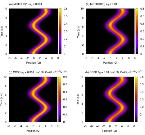
This 1-body density is shown as a function of position and time in Fig. 3 for interaction strengths λ0 = 0.001

in (i) and λ0 = 0.01 in (ii), with the MCTDHB

cal-culations in panel (a) and CCSB calcal-culations in panel (b). The MCTDHB calculations use 1 orbital for the

λ0 = 0.001 case, and 3 orbitals for the λ0 = 0.01 case,

labelled as MCTDHB(1) and MCTDHB(3), respectively. The CCSB calculations use K = 150 configurations for both theλ0 = 0.001 and λ0 = 0.01 cases, with Ω = 26

harmonic oscillator levels for the λ0 = 0.001 case and

Ω = 25 harmonic oscillator levels for theλ0= 0.01 case,

with the compression parametersσ(α>0)_{as mentioned in}

the previous section. It can be seen that the MCTDHB and CCSB calculations of the 1-body density compare well to one another, illustrating the oscillations in the bosonic cloud due to the trap displacement.

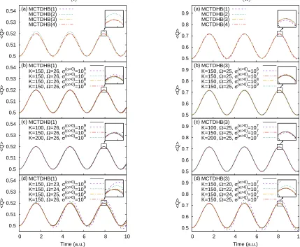
As well as the density being subject to oscillations as a function of the trap displacement, it also exhibits breath-ing oscillations, which may not be immediately apparent from Fig.3. To illustrate these, we plot the variance in the 1-body density as a function of time

hQi=

Z

Q2ρ(Q) dQ−

Z

Qρ(Q) dQ

2

, (40)

which is shown in Fig.4, with the interaction strengths

λ0 = 0.001 in (i) and λ0 = 0.01 in (ii). It can

immedi-ately be seen that the stronger interaction strength pro-duces larger breathing oscillations, which is not as easy to see in Fig.3. Furthermore, the breathing oscillations in Fig.4serve to determine the convergence of the meth-ods: MCTDHB with respect to the number of orbitals; and CCSB with respect toσ(α>0)_,_K_{, and Ω. A portion}

of the peak of the density variance at∼8 a.u. is high-lighted to clearly illustrate any discrepancies that may be difficult to distinguish. As with Application 1, the accuracy and convergence of the CCSB calculation may also be determined from the conservation of norm and particle number, which is shown in Fig.5.

Forλ0= 0.001, the MCTDHB calculations using 1, 3,

(11)

[image:11.612.77.544.66.503.2]

(i) (ii)

FIG. 3: Space-time representation of the evolution of the 1-body density for (a) MCTDHB and (b) CCSB calculations of Application 2 with interaction strengths (i)λ0= 0.001 and (ii) λ0= 0.01.

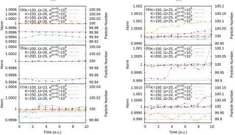
In panel (b) of Fig.4(i)we alter the value of the com-pression parameter σ(α>0)_{, whilst keeping the number}

of configurations fixed at K = 150, and the number of harmonic oscillator levels fixed at Ω = 26. There ap-pears to be little difference in the breathing oscillations for different values of σ(α>0)_{, although the highlighted}

peak at ∼8 .a.u. demonstrates small discrepancies be-tween the MCTDHB calculation and σ(α>0) _{= 10}6 _and

σ(α>0)_{= 10}7_{, whilst}_σ(α>0)_{= 10}8 _and_σ(α>0)_{= 10}9

su-perimpose on the MCTDHB result. The conservation of norm and particle number for different values ofσ(α>0)

is shown in panel (a) of Fig.5(i), whereσ(α>0)_{= 10}8_and

σ(α>0) _{= 10}9 _{superimpose upon a value of the norm of}

1, and particle number 100, as should be expected. We

keepσ(α>0)_{= 10}9_{for the remaining calculations. This is}

much larger than the compression parameter used in Ap-plication 1, however much fewer configurations are used in this application, and the compression parameter nec-essary also depends upon the problem studied, and how the dynamics affect the motion of the basis.

In panel (c) of Fig.4(i) we alter the value ofK whilst keeping σ(α>0) _{and Ω fixed. Altering the value of the}

compression parameter for different values ofK was not necessary like in Application 1, as a stable basis was able to be formed. We observe very little discrepancy between the different CCSB calculations and MCTDHB, and the norm and particle number conservation forK= 150 and

(12)

(i)

0.5 0.51 0.52 0.53 0.54

0 2 4 6 8 10

(d)

<Q>

Time (a.u.) MCTDHB(1)

K=150, Ω=23, σ(α>0)=109 K=150, Ω=24, σ(α>0)=109 K=150, Ω=25, σ(α>0)=109 K=150, Ω=26, σ(α>0)=109 0.5

0.51 0.52 0.53 0.54 (c)

<Q>

MCTDHB(1)

K=100, Ω=26, σ(α>0)=109 K=150, Ω=26, σ(α>0)=109 K=200, Ω=26, σ(α>0)=109 0.5

0.51 0.52 0.53 0.54 (b)

<Q>

MCTDHB(1)

0.51 0.52 0.53 0.54 (a)

<Q>

MCTDHB(1) MCTDHB(2) MCTDHB(3) MCTDHB(4)

(ii)

0.5 0.6 0.7 0.8 0.9

0 2 4 6 8 10

(d)

<Q>

Time (a.u.) MCTDHB(3)

0.6 0.7 0.8 0.9 (c)

<Q>

MCTDHB(3)

K=100, Ω=25, σ(α>0)=107 K=150, Ω=25, σ(α>0)=107 K=200, Ω=25, σ(α>0)=107 0.5

0.6 0.7 0.8 0.9 (b)

<Q>

MCTDHB(3)

0.6 0.7 0.8 0.9 (a)

<Q>

[image:12.612.79.508.58.411.2]

MCTDHB(1) MCTDHB(2) MCTDHB(3) MCTDHB(4)

FIG. 4: Variance of the 1-body densityhQifor Application 2 with two-body interaction strength (i)λ0= 0.001 and

(ii)λ0= 0.01. In the (a) panels MCTDHB calculations with different numbers of orbitals are shown, and the

converged result is used to compare to CCSB calculations with different values of (b) compression parameter for coherent state sampling of the harmonic oscillator levels with zero initial occupationσ(α>0)_{, (c) configurations}_K

and (d) harmonic oscillator levels in the basis Ω.

therefore regardK= 150 as being fully converged. In panel (d) of Fig. 4(i) we alter the value of Ω and keepKandσ(α>0)_{fixed. As with the above, altering the}

value ofσ(α>0) _{was not necessary as a stable basis was}

able to be formed each time. Larger discrepancies be-tween the CCSB calculations and the MCTDHB result are seen with in this panel, indicating that the choice of Ω has the largest influence on this calculation. The results for Ω = 25 and Ω = 26 superimpose, indicating that the calculation is converged by this point. The con-servation of norm and particle number for both of these calculations is also similar in panel (c) of Fig.5(i).

Turning to the larger interaction strength ofλ0= 0.01,

we follow the same approach as above in determining the accuracy and convergence of the calculations. Initially, in panel (a) of Fig.4(i) the MCTDHB calculations with 1 and 2 orbitals exhibit minor differences to those with 3 and 4 orbitals, shown in the highlighted portion of the figure, so we regard the MCTDHB(3) calculation as our

fully converged reference point. At this level of interac-tion strength, an above mean-field descripinterac-tion is therefore necessary. We admit that the discrepancy between these MCTDHB calculations is not very large, however a sim-ilar study in Ref. [31] also illustrated minor differences in breathing dynamics for MCTDHB calculations with different numbers of orbitals.

In panel (b) of Fig.4(ii)we alter the value of the com-pression parameter σ(α>0)_{, whilst keeping the number}

of configurations fixed at K = 150, and the number of harmonic oscillator levels fixed at Ω = 25. All the calcu-lations superimpose, and there is even less discrepancy than in theλ0= 0.001 case. For the remaining

calcula-tions we choose a compression parameter ofσ(α>0)_{= 10}7

as this demonstrates the best norm and particle number conservation in panel (a) of Fig.5(ii).

In panel (c) of Fig.4(ii)we alter the value ofKwhilst keepingσ(α>0) _{and Ω fixed. There are minor differences}

(13)

(i)

0.9998 1 1.0002 1.0004

0 2 4 6 8 10 99.98 100 100.02 100.04 (c)

Norm

Particle Number

Time (a.u.) K=150, Ω=23, σ(α>0)=109 K=150, Ω=24, σ(α>0)=109 K=150, Ω=25, σ(α>0)=109 K=150, Ω=26, σ(α>0)=109 0.9994

0.9996 0.9998 1 1.0002 1.0004

99.94 99.96 99.98 100 100.02 100.04 (b)

Norm

Particle Number

K=100, Ω=26, σ(α>0)=109 K=150, Ω=26, σ(α>0)=109 K=200, Ω=26, σ(α>0)=109 0.9992

0.9994 0.9996 0.9998 1 1.0002 1.0004 1.0006

99.92 99.94 99.96 99.98 100 100.02 100.04 100.06 (a)

Norm

Particle Number

K=150, Ω=26, σ(α>0)=106 K=150, Ω=26, σ(α>0)=107 K=150, Ω=26, σ(α>0)=108 K=150, Ω=26, σ(α>0)=109

(ii)

0.999 0.9995 1 1.0005 1.001 1.0015

0 2 4 6 8 10 99.9 99.95 100 100.05 100.1 100.15 (c)

Norm

Particle Number

Time (a.u.) K=150, Ω=20, σ(α>0)=107 K=150, Ω=22, σ(α>0)=107 K=150, Ω=24, σ(α>0)=107 K=150, Ω=25, σ(α>0)=107 0.999

0.9995 1 1.0005 1.001

99.9 99.95 100 100.05 100.1 (b)

Norm

Particle Number

K=100, Ω=25, σ(α>0)=107 K=150, Ω=25, σ(α>0)=107 K=200, Ω=25, σ(α>0)=107 0.9995

1 1.0005 1.001 1.0015 1.002

99.95 100 100.05 100.1 100.15 100.2 (a)

Norm

Particle Number

[image:13.612.80.542.58.323.2]

K=150, Ω=25, σ(α>0)=106 K=150, Ω=25, σ(α>0)=107 K=150, Ω=25, σ(α>0)=108 K=150, Ω=25, σ(α>0)=109

FIG. 5: Norm (dashed/dotted lines without circles) and particle number (dashed/dotted lines with circles) for CCSB calculations of Application 2 with two-body interaction strength (i)λ0= 0.001 and (ii)λ0= 0.01 with

different values of (a) compression parameter for coherent state sampling of the harmonic oscillator levels with zero initial occupation σ(α>0)_{, (b) configurations}_K _{and (c) harmonic oscillator levels in the basis Ω.}

K = 200 calculations, the latter of which superimpose on the MCTDHB result. The norm and particle number conservation of theK = 150 andK = 200 calculations are very similar in panel (b) of Fig. 5(ii), therefore we regard theK= 150 result as being fully converged.

In panel (d) of Fig. 4(ii) we alter the value of Ω and keep K and σ(α>0) _{fixed. As with the} _λ

0 = 0.001

cal-culations, this has the largest effect on the breathing os-cillations, with Ω = 20 and Ω = 22 being insufficient to describe them accurately, whilst the Ω = 24 and Ω = 25 cases superimpose upon the MCTDHB result. The norm and particle number conservation of the Ω = 24 result, shown in panel (c) of Fig. 5(ii) is not as good as the Ω = 25 result, which is why we choose the latter as our most accurate calculation.

The above demonstrates that CCSB is able to repro-duce MCTDHB calculations in both the mean field and multi orbital fully quantum regimes, with similar levels of theory for the CCSB calculations in each regime. We have also shown that the method converges appropriately with respect to theKand Ω parameters, this it is stable with respect to norm and particle number conservation, and that appropriate choice of the compression parame-terσ(α>0)_{for initial sampling of the coherent state basis}

is necessary, like in Application 1.

V. CONCLUSIONS

In this work the CCS method has been straight-forwardly applied to investigation of indistinguishable bosons, as MCTDH and ML-MCTDH have been, and the method dubbed CCSB. Instead of the coherent state basis functions being used to represent individual par-ticles like in the standard distinguishable representation of CCS, in CCSB they are used as a basis for number occupation of quantum states in the second quantisation Fock state formalism.

(14)

possibil-ity of the method studying multi-atomic Bose-Einstein condensates [64], spinor Bose-Einstein condensates [65], dark-bright solitons [66], and Bose-polarons [67]. The previously studied 20D, quadratic system-bath coupling with constant λ = 0.1 case [72–75, 78, 79] was investi-gated, and the second quantised bath required Ω = 5 harmonic oscillator levels in the basis, thus the dimen-sionality of the problem was reduced from 20 to 6. The CCSB calculation was in much better agreement with a benchmark result [79] on the system than all other meth-ods that have studied the problem.

In the second example, a model Hamiltonian for a sys-tem of 100 bosons in a shifted harmonic trap was stud-ied, the 1-body density has been calculated, as well as its variance, to demonstrate the breathing oscillations of the density. Matrix elements of 2-body operators had to be calculated, as is common for interacting conden-sates, and these may be computed analytically by CCSB. The density oscillations were calculated at two different two-body interaction strengths and compared to MCT-DHB benchmark calculations. The weaker interaction strength was able to be described by MCTDHB with 1 orbital, such that it was equivalent to the GPE mean-field theory, whilst the stronger interaction strength required MCTDHB with 3 orbitals, and was thus fully quantum, taking correlations into account and going beyond the mean-field approach. CCSB was able to reproduce both results with similar levels of theory, providing motivation for further study on more challenging Bose-Einstein con-densate systems. In particular, future avenues of research for CCSB in this vein include more complicated Bose-Einstein condensate problems, such as that in Ref. [22] of a condensate in a single well trap that is deformed into a double well, like that observed in experimental bosonic Josephson junctions [70, 71]. We also wish to consider condensates in multi-well traps, such as a multi-site

ver-sion of the Bose-Hubbard model studied in Ref. [61], and other interesting systems that have previously been stud-ied by ML-MCTDHB [45–52].

Both applications have demonstrated that the CCSB method converges with the number of configurationsK

and number of quantum states included in the basis Ω. We have also demonstrated that appropriate sampling of the initial coherent states via a compression parameter

σis necessary to ensure a reliable and accurate calcula-tion. Further developments of the method that we envis-age in future include development of methods to generate initial conditions, as imaginary time propagation is un-stable with trajectories; incorporation of SU(n) coherent states, as demonstrated in Ref. [83]; and the combination of the method with one to treat identical fermions [84] to study Bose-Fermi mixtures, as has been carried out by MCTDH [85] and ML-MCTDH [86] previously.

VI. ACKNOWLEDGEMENTS

J.A.G. has been supported by EPSRC grant EP/N007549/1, as well as the University Research Schol-arship from the University of Leeds, and funding from the School of Chemistry, University of Leeds. D.V.S acknowl-edges the support of the EPSRC, grant EP021123/1. J.A.G. would like to thank A. Streltsov for demonstra-tion of the use of the MCTDHB program, alongside helpful discussions. J.A.G would also like to thank L. Chen for reading through the manuscript and suggest-ing modifications. J.A.G. and D.V.S gratefully acknowl-edge V. Batista, S. Habershon, and M. Saller for pro-viding their data. This work was undertaken on ARC2 and ARC3, part of the High Performance Computing fa-cilities at the University of Leeds, UK. Data generated in this work that is shown in the figures may be found at https://doi.org/10.5518/595, along with the program code used to generate the data.

Appendix A: Second Quantisation and Normal Ordering of Hamiltonian for Application 1

Using the definition of a second quantised Hamiltonian in Eq.17in the main text, Eq.18may be written as

ˆ

H = pˆ

(m=1)2

2 −

ˆ

q(m=1)2

2 +

ˆ

q(m=1)4

16η +





Ω

X

α,β=0

hα|Pˆ

2

2 + ˆ Q2

2 |βiaˆ

(α)†_ˆ_a(β)



+

λqˆ(m=1)

2





Ω

X

α,β=0

hα|Qˆ2_|βiˆa(α)†_ˆ_a(β)





= pˆ

(m=1)2

2 −

ˆ

q(m=1)2

2 +

ˆ

q(m=1)4

16η +

" _Ω X

α=0

hα|Pˆ

2

2 + ˆ Q2

2 |αiˆa

(α)†_ˆ_a(α)

#

+λqˆ

(m=1)

2





Ω

X

α,β=0

Q(α,β)2ˆa(α)†ˆa(β)





= pˆ

(m=1)2

2 −

ˆ

q(m=1)2

2 +

ˆ

q(m=1)4

16η +

" _Ω X

α=0

ǫ(α)aˆ(α)†ˆa(α)

#

+λqˆ

(m=1)

2





Ω

X

α,β=0

Q(α,β)2ˆa(α)†ˆa(β)



.

(A1)

The quantum states|αiand|βiare those of the harmonic oscillator withαandβnumbers of quanta, and the equality on the second line for hα|Pˆ2

2 + ˆ

Q2

2 |βi follows because this is non-zero with eigenvalue ǫ(α) only when α= β. The

(15)

result is achieved. The position and momentum operators of the tunnelling mode have explicitly been labelled with (m= 1) to distinguish them from theαlabelling scheme of the second quantised bath modes.

The matrixQ(α,β)2

is evaluated as

hα|Qˆ2_|βi=

               1 2 p

(α+ 2)(α+ 1) ifα=β−2

1 2

p

α(α−1) ifα=β+ 2

ǫ(α) ifα=β

0 otherwise.

(A2)

As this matrix is non-zero only for quanta α=β andα=β±2, and we may say that all bath modes are initially in the ground harmonic oscillator level (α= 0) as they are at the origin in distinguishable representation (previously assumed in the benchmark calculation [79]), only harmonic oscillator levels with even numbers of quanta will be included and the bottom line of Eq.A1is written as

ˆ

H = pˆ

(m=1)2

2 −

ˆ

q(m=1)2

2 +

ˆ

q(m=1)4

16η +

" _Ω X

α=0

ǫ(2α)aˆ(2α)†aˆ(2α)

#

+λqˆ

(m=1) 2   Ω X α,β=0

Q(2α,2β)2aˆ(2α)†ˆa(2β)



. (A3)

The relationship between the creation and annihilation operators and ˆq and ˆpgiven in Eq. 3 may then be used in Eq.A3alongside the relationships in Eqs.2 and6to give Eq.19.

Appendix B: Second Quantisation of Hamiltonian for Application 2

Using the definition of a second quantised Hamiltonian in Eq.17in the main text, Eq.32may be written as

ˆ

H =

Ω

X

α,β=0

hα|Pˆ

2

2 + ˆ Q2

2 |βiˆa

(α)†_a_ˆ(β)

−

Ω

X

α,β=0

hα|ξQˆ_|βiˆa(α)†ˆa(β)+

Ω

X

α,β=0

hα|ξ

2

2 |βiaˆ

(α)†_ˆ_a(β)

+1 2

Ω

X

α,β,γ,ζ=0

hα, β|λ0δ(Q−Q′)|γ, ζiâ(α)†aˆ(β)†â(ζ)â(γ)

=

Ω

X

α=0

hα|Pˆ

2

2 + ˆ Q2

2 |αiˆa

(α)†_ˆ_a(α)

−

Ω

X

α,β=0

hα|ξQˆ_|βiˆa(α)†ˆa(β)+

Ω

X

α=0

hα|ξ

2

2 |αiˆa

(α)†_ˆ_a(α)

+1 2

Ω

X

α,β,γ,ζ=0

hα, β|λ0δ(Q−Q′)|γ, ζiâ(α)†aˆ(β)†â(ζ)â(γ)

=

Ω

X

α=0

ǫ(α)_a_ˆ(α)†_ˆ_a(α)₋ Ω

X

α,β=0

ξQ(α,β)_ˆ_a(α)†_ˆ_a(β)₊ Ω

X

α=0

ξ2

2aˆ

(α)†_ˆ_a(α)₊1

2

Ω

X

α,β,γ,ζ=0

λ0δ(α,β,γ,ζ)â(α)†aˆ(β)†â(ζ)â(γ).

(B1)

The relationships in Eqs. 2and 6may then be used with Eq. B1to give Eq.34. In Eq.B1,ǫ(α)_{is the eigenvalue of}

the harmonic oscillator for state|αi, and Q(α,β)_{is a matrix given by}

Q(α,β)=hα|Qˆ_|βi=

     pα

2 α=β+ 1

q

β

2 β =α+ 1

0 otherwise.

. (B2)

Evaluation of theδ(α,β,γ,ζ)_{matrix is slightly more involved, as it is required to solve the integral}

δ(α,β,γ,ζ)=hα, β|δ(Q₋Q′)|γ, ζi

=

Z +∞

−∞

Z +∞

−∞ 1

√

2α_α_!

₁

π

1/4

e−Q2/2He(α)(Q)p1

2β_β_!

₁

π

1/4

e−Q′2/2He(β)(Q′)

×δ(Q−Q′)√1

2γ_γ_!

₁

π

1/4

e−Q2/2_He(γ)_(Q) 1

p

2ζ_ζ_!

₁

π

1/4

e−Q′2/2_He(ζ)_(Q′_{) dQ}_dQ′

(16)

whereHe(α)(Q) is a Hermite polynomial of orderα. However, an analytic solution is possible, and the above may be simplified using the relationship

Z +∞

−∞

f(x′₎_δ₍_x₋_x′_{) d}_x′₌_f₍_x₎_, _(B4)

and like terms collated to obtain

δ(α,β,γ,ζ)= 1

πp2(α+β+γ+ζ)_α_!_β_!_γ_!_ζ_!

Z +∞

−∞

e−2Q2He(α)(Q)He(β)(Q)He(γ)(Q)He(ζ)(Q) dQ. (B5)

This will only be non-zero if the integrand is an even function, so the product of Hermite polynomials can only have even powers ofQ

δ(α,β,γ,ζ)= 1

πp2α+β+γ+ζ_α_!_β_!_γ_!_ζ_!

Z +∞

−∞ e−2Q2

(α+β+γ+ζ)/2

X

τ=0

c2τQ2τdQ (B6)

wherec2τ is a constant obtained from the product of Hermite polynomial coefficients. Using the following identity

Z +∞

−∞

x2ne−12ax 2

=

r

2π a

1

an(2n−1)!! forn >0 (B7)

combined with a Gaussian integral forτ= 0, Eq.B6can be evaluated as

δ(α,β,γ,ζ)= 1

πp2α+β+γ+ζ_α_!_β_!_γ_!_ζ_!



 r

π

2c0+

(α+β+γ+ζ)/2

X

τ=1

c2τ

r

π

2 1

4τ(2τ−1)!!



. (B8)

We note that an alternative method of calculating theδ(α,β,γ,ζ)_{matrix elements exists using Gauss-Hermite}

quadra-ture [87], however our approach was sufficiently efficient.

[1] M. H. Anderson, J. R. Ensher, M. R. Matthews, C. E. Wieman, and E. A. Cornell,Science269, 198 (1995). [2] C. C. Bradley, C. A. Sackett, J. J. Tollett, and R. G.

Hulet,Physical Review Letters75, 1687 (1995). [3] K. B. Davis, M. O. Mewes, M. R. Andrews, N. J. van

Druten, D. S. Durfee, D. M. Kurn, and W. Ketterle,

Physical Review Letters75, 3969 (1995).

[4] C. Orzel, A. K. Tuchman, M. L. Fenselau, M. Yasuda, and M. A. Kasevich, Science291, 2386 (2001).

[5] M. Albiez, R. Gati, J. F¨olling, S. Hunsmann, M. Cris-tiani, and M. K. Oberthaler, Physical Review Letters 95, 010402 (2005).

[6] S. Levy, E. Lahoud, I. Shomroni, and J. Steinhauer,

Nature449, 579 (2007).

[7] M. R. Matthews, B. P. Anderson, P. C. Haljan, D. S. Hall, C. E. Wieman, and E. A. Cornell,Physical Review Letters83, 2498 (1999).

[8] K. W. Madison, F. Chevy, W. Wohlleben, and J. Dal-ibard,Physical Review Letters84, 806 (2000).

[9] S. Burger, K. Bongs, S. Dettmer, W. Ertmer, K. Seng-stock, A. Sanpera, G. V. Shlyapnikov, and M. Lewen-stein,Physical Review Letters83, 5198 (1999).

[10] J. Denschlag, J. E. Simsarian, D. L. Feder, C. W. Clark, L. A. Collins, J. Cubizolles, L. Deng, E. W. Hagley,

K. Helmerson, W. P. Reinhardt, S. L. Rolston, B. I. Schneider, and W. D. Phillips,Science287, 97 (2000). [11] E. P. Gross,Nuovo Cimento20, 454 (1961).

[12] L. P. Pitaevskii, Soviet Physics JETP-USSR 13, 451 (1961).

[13] A. Smerzi, S. Fantoni, S. Giovanazzi, and S. R. Shenoy,

Physical Review Letters79, 4950 (1997).

[14] V. M. P´erez-Garc´ıa, H. Michinel, J. I. Cirac, M. Lewen-stein, and P. Zoller,Physical Review A56, 1424 (1997). [15] S. Raghavan, A. Smerzi, S. Fantoni, and S. R. Shenoy,

Physical Review A59, 620 (1999).

[16] W. Bao, D. Jaksch, and P. A. Markowich,Journal of Computational Physics187, 318 (2003).

[17] Z. X. Liang, Z. D. Zhang, and W. M. Liu, Physical Review Letters94, 050402 (2005).

[18] D. Ananikian and T. Bergeman,Physical Review A73, 013604 (2006).

[19] A. J. Leggett,Reviews of Modern Physics73, 307 (2001). [20] A. Minguzzi, S. Succi, F. Toschi, M. Tosi, and P. Vignolo,

Physics Reports395, 223 (2004).

[21] A. I. Streltsov, O. E. Alon, and L. S. Cederbaum, Phys-ical Review Letters99, 030402 (2007).

(17)

[24] A. I. Streltsov, O. E. Alon, and L. S. Cederbaum, Phys-ical Review A80, 043616 (2009).

[25] A. I. Streltsov, O. E. Alon, and L. S. Cederbaum,Journal of Physics B42, 091004 (2009).

[26] A. U. J. Lode, A. I. Streltsov, O. E. Alon, H.-D. Meyer, and L. S. Cederbaum, Journal of Physics B 42, 044018 (2009).

[27] K. Sakmann, A. I. Streltsov, O. E. Alon, and L. S. Ceder-baum,Physical Review Letters103, 220601 (2009). [28] K. Sakmann, A. I. Streltsov, O. E. Alon, and L. S.

Ceder-baum,Physical Review A82, 013620 (2010).

[30] A. I. Streltsov, K. Sakmann, O. E. Alon, and L. S. Ceder-baum,Physical Review A83, 043604 (2011).

[31] A. U. J. Lode, K. Sakmann, O. E. Alon, L. S. Cederbaum, and A. I. Streltsov,Physical Review A86, 063606 (2012). [32] A. I. Streltsov,Physical Review A88, 041602(R) (2013). [33] R. Beinke, S. Klaiman, L. S. Cederbaum, A. I. Streltsov, and O. E. Alon,Physical Review A92, 043627 (2015). [34] L. Cao, S. Kr¨onke, O. Vendrell, and P. Schmelcher,

Jour-nal of Chemical Physics139, 134103 (2013).

[35] S. Kr¨onke, L. Cao, O. Vendrell, and P. Schmelcher,New Journal of Physics15, 063018 (2013).

[36] J. M. Schurer, A. Negretti, and P. Schmelcher,Physical Review Letters119, 063001 (2017).

[37] K. Keiler and P. Schmelcher,New Journal of Physics20, 103042 (2018).

[38] S. I. Mistakidis, A. G. Volosniev, N. T. Zinner, and P. Schmelcher,ArXiv e-prints (2018), arXiv:1809.01889. [39] S. Mistakidis, G. Katsimiga, G. Koutentakis, T. Busch, and P. Schmelcher, ArXiv e-prints (2018), arXiv:1811.10702.

[40] G. C. Katsimiga, S. I. Mistakidis, G. M. Koutentakis, P. G. Kevrekidis, and P. Schmelcher,Physical Review A 98, 013632 (2018).

[41] S. I. Mistakidis, G. C. Katsimiga, P. G. Kevrekidis, and P. Schmelcher,New Journal of Physics20, 043052 (2018). [42] G. C. Katsimiga, G. M. Koutentakis, S. I. Mistakidis, P. G. Kevrekidis, and P. Schmelcher, New Journal of Physics19, 073004 (2017).

[43] S. Kr¨onke and P. Schmelcher, Physical Review A 91, 053614 (2015).

[44] G. C. Katsimiga, S. I. Mistakidis, G. M. Koutentakis, P. G. Kevrekidis, and P. Schmelcher, New Journal of Physics19, 123012 (2017).

[45] S. I. Mistakidis, L. Cao, and P. Schmelcher,Journal of Physics B: Atomic, Molecular and Optical Physics 47, 225303 (2014).

[46] S. I. Mistakidis, L. Cao, and P. Schmelcher, Physical Review A91, 033611 (2015).

[47] S. I. Mistakidis, T. Wulf, A. Negretti, and P. Schmelcher,

Journal of Physics B: Atomic, Molecular and Optical Physics48, 244004 (2015).

[48] S. I. Mistakidis and P. Schmelcher, Physical Review A 95, 013625 (2017).

[49] G. M. Koutentakis, S. I. Mistakidis, and P. Schmelcher,

Physical Review A95, 013617 (2017).

[50] J. Neuhaus-Steinmetz, S. I. Mistakidis, and P. Schmelcher,Physical Review A95, 053610 (2017). [51] S. Mistakidis, G. Koutentakis, and P. Schmelcher,

Chemical Physics509, 106 (2018).

[52] T. Plaßmann, S. I. Mistakidis, and P. Schmelcher, Jour-nal of Physics B: Atomic, Molecular and Optical Physics 51, 225001 (2018).

[53] H.-D. Meyer, U. Manthe, and L. Cederbaum,Chemical Physics Letters165, 73 (1990).

[54] H. Wang and M. Thoss,Journal of Chemical Physics119, 1289 (2003).

[55] U. Manthe, Journal of Chemical Physics 128, 164116 (2008).

[56] D. V. Shalashilin and M. S. Child,Journal of Chemical Physics113, 10028 (2000).

[57] D. V. Shalashilin and M. S. Child,Chemical Physics304, 103 (2004).

[60] L. Simon and W. T. Strunz, Physical Review A 89, 052112 (2014).

[61] S. Ray, P. Ostmann, L. Simon, F. Grossmann, and W. T. Strunz,Journal of Physics A: Mathematical and Theo-retical49, 165303 (2016).

[62] M. S. Child and D. V. Shalashilin,Journal of Chemical Physics118, 2061 (2003).

[64] G. Modugno, M. Modugno, F. Riboli, G. Roati, and M. Inguscio,Physical Review Letters89, 190404 (2002). [65] Y. Kawaguchi and M. Ueda,Physics Reports 520, 253

(2012).

[66] C. Becker, S. Stellmer, P. Soltan-Panahi, S. D¨orscher, M. Baumert, E.-M. Richter, J. Kronj¨ager, K. Bongs, and K. Sengstock,Nature Physics4, 496 (2008).

[67] M. Bruderer, A. Klein, S. R. Clark, and D. Jaksch, Phys-ical Review A76, 011605(R) (2007).

[68] M. Greiner, O. Mandel, T. Esslinger, T. W. H¨ansch, and I. Bloch,Nature415, 39 (2002).

[69] D. Jaksch and P. Zoller, Annals of Physics 315, 52 (2005).

[70] R. Gati, M. Albiez, J. F¨olling, B. Hemmerling, and M. Oberthaler,Applied Physics B82, 207 (2006). [71] R. Gati and M. K. Oberthaler, Journal of Physics B:

Atomic, Molecular and Optical Physics40, R61 (2007). [72] Y. Wu and V. S. Batista,Journal of Chemical Physics

121, 1676 (2004).

[73] P. A. J. Sherratt, D. V. Shalashilin, and M. S. Child,

Chemical Physics322, 127 (2006).

[74] S. Habershon,Journal of Chemical Physics136, 054109 (2012).

[75] M. A. C. Saller and S. Habershon,Journal of Chemical Theory and Computation13, 3085 (2017).

[76] J. P. Alborzpour, D. P. Tew, and S. Habershon,Journal of Chemical Physics145, 174112 (2016).

[77] T. Murakami and T. J. Frankcombe,Journal of Chemical Physics149, 134113 (2018).

[78] J. A. Green, A. Grigolo, M. Ronto, and D. V. Shalashilin,

Journal of Chemical Physics144, 024111 (2016). [79] J. A. Green and D. V. Shalashilin,Chemical Physics

Let-ters641, 173 (2015).

[80] A. I. e. a. Streltsov, “The multiconfigurational time-dependent hartree for bosons package,”

Http://mctdhb.org.

(18)

[82] K. Sakmann, A. I. Streltsov, O. E. Alon, and L. S. Ceder-baum,Physical Review A89, 023602 (2014).

[83] A. Grigolo, T. F. Viscondi, and M. A. M. de Aguiar,

Journal of Chemical Physics 144, 094106 (2016). [84] D. V. Shalashilin, Journal of Chemical Physics 148,

194109 (2018).

[85] O. E. Alon, A. I. Streltsov, and L. S. Cederbaum,Journal

of Chemical Physics127, 154103 (2007).

[86] L. Cao, V. Bolsinger, S. I. Mistakidis, G. M. Koutentakis, S. Kr¨onke, J. M. Schurer, and P. Schmelcher,Journal of Chemical Physics147, 044106 (2017).

[87] M. Edwards, R. J. Dodd, C. W. Clark, and K. Burnett,