Two-step semiparametric empirical likelihood inference

White Rose Research Online URL for this paper:

http://eprints.whiterose.ac.uk/138992/

Version: Accepted Version

Article:

Bravo, Francesco orcid.org/0000-0002-8034-334X, Escanciano, Juan Carlos and van

Keilegom, Ingrid (Accepted: 2018) Two-step semiparametric empirical likelihood inference.

Annals of Statistics. ISSN 0090-5364 (In Press)

eprints@whiterose.ac.uk https://eprints.whiterose.ac.uk/

Reuse

Items deposited in White Rose Research Online are protected by copyright, with all rights reserved unless indicated otherwise. They may be downloaded and/or printed for private study, or other acts as permitted by national copyright laws. The publisher or other rights holders may allow further reproduction and re-use of the full text version. This is indicated by the licence information on the White Rose Research Online record for the item.

Takedown

If you consider content in White Rose Research Online to be in breach of UK law, please notify us by

TWO-STEP SEMIPARAMETRIC EMPIRICAL LIKELIHOOD INFERENCE

By Francesco Bravo‡ , Juan Carlos Escanciano ∗,§ and Ingrid Van Keilegom †,¶

University of York‡, Universidad Carlos III de Madrid § and KU Leuven¶

In both parametric and certain nonparametric statistical mod-els, the empirical likelihood ratio satisfies a nonparametric version of Wilks’ theorem. For many semiparametric models, however, the com-monly used two-step (plug-in) empirical likelihood ratio is not asymp-totically distribution-free, that is, its asymptotic distribution contains unknown quantities and hence Wilks’ theorem breaks down. This ar-ticle suggests a general approach to restore Wilks’ phenomenon in two-step semiparametric empirical likelihood inferences. The main insight consists in using as the moment function in the estimating equation the influence function of the plug-in sample moment. The proposed method is general; it leads to a chi-squared limiting distribu-tion with known degrees of freedom; it is efficient; it does not require undersmoothing; and it is less sensitive to the first-step than alter-native methods, which is particularly appealing for high-dimensional settings. Several examples and simulation studies illustrate the gen-eral applicability of the procedure and its excellent finite sample per-formance relative to competing methods.

1. Introduction. Since its introduction as a nonparametric likelihood alternative to likelihood-type bootstrap methods for constructing confidence regions, Owen’s ([55,56,57]) empirical likelihood (EL henceforth) has been used extensively in both statistics and econometrics. Such popularity is jus-tified by the appealing theoretical properties of EL confidence regions: they tend to be more concentrated in places where the density of the parameter estimator is greatest; they can be Bartlett corrected ([22] for the so-called smooth function model, [10] for exactly identified estimating equations mod-els, [16] for exactly identified estimating equations models with nuisance pa-rameters and [17] for over-identified estimating equations models); they do

∗_{Juan Carlos Escanciano gratefully acknowledges support by the Ministerio Economia}

y Competitividad (Spain), ECO2017-86675-P & MDM 2014-0431, and by Comunidad de Madrid (Spain), MadEco-CM S2015/HUM-3444.

†_{Ingrid Van Keilegom acknowledges financial support from the European Research}

Council (2016-2021, Horizon 2020/ERC grant agreement No. 694409). MSC 2010 subject classifications:Primary 62M10; secondary 62G10

Keywords and phrases: Empirical likelihood, Semiparametric inference, High-dimensional parameters, Wilks’ phenomenon

not require estimation of scale (internal studentization) and skewness; and finally, they are range preserving and transformation respecting. Further-more, [21] show that in linear exponential families empirical and parametric likelihood surfaces are quite close in terms of their asymptotic distribution. Specifically, the chi-squared approximations to the distributions of the em-pirical and likelihood ratios, as well as the asymptotic normality of their signed squared root differ in terms of order O(n−1), wheren is the sample size. See [57] for a comprehensive review of these properties and a number of applications geared mainly towards finite-dimensional statistical models. More recently the EL method has been used in nonparametric and semi-parametric models. For nonsemi-parametric models [25] considered sieve empir-ical likelihood for testing nonparametric hypotheses about nonparametric functions, and showed that an appropriately rescaled sieve EL ratio test has an asymptotic chi-squared calibration, with the scaling constant and de-grees of freedom being independent of nuisance parameters, in other words the so-called Wilks’ phenomenon ([80]) (i.e. the likelihood ratio statistic is asymptotically distribution-free and converges to a chi-squared distribution) holds for the EL. In semiparametric models [7] has shown that Wilks’ The-orem also holds in certain “highly smooth” cases, see Remark 2.3 in [32] for discussion.

For semiparametric models the most popular method uses a two-step (plug-in) procedure in which the first-step estimator replaces the infinite-dimensional nuisance parameter, while in the second step the plug-in EL ratio is used to obtain inferences for the finite-dimensional parameter of interest. This two-step semiparametric EL approach has been considered by a number of authors, including [75] for partially linear models, [86] for single-index models, [89, 81, 30] for various censored regression problems, [77,78,79,76,74,70] for various missing data problems, and [7,48,49,12,

11] for other semiparametric problems. [18, 88] provide recent surveys on EL inference in the context of semiparametric regression models.

semiparametric model in each bootstrap iteration, and thus are computa-tionally very expensive. The second proposal consists in adjusting the EL by a scale factor such that the adjusted (or rescaled) EL ratio is asymptotically pivotal. [76] proposed a specific scale factor; more general adjustments have been proposed by [86, 84, 12]. Although sometimes effective, these adjust-ments typically involve explicit estimation of various covariance matrices, which can be very complicated to be carried out in practice. Furthermore the internal studentization property of EL is not exploited and this can neg-atively affect the finite sample performance of the resulting EL statistic. The third proposal exploits that in some specific cases it is possible to modify the original estimating equation in such a way that the effect of the first-step estimation is removed. This approach has been called in the EL literature “bias-reduced or bias-corrected EL”. A review of papers using this approach is provided in Section 2.3. As shown first by [91] in the context of a partially linear single-index model, this approach has the additional advantage of not requiring undersmoothing (the bias of the first-step going to zero faster than its standard deviation), much in contrast to bootstrap and adjusted based methods, but it is not clear how the method works, that is, how the modified estimating equations were obtained in the first place for the specific models considered, and how similar estimating equations could be built for other semiparametric models.

This leads us to the main contribution of this article, which is to propose a theoretical justification of “bias-corrected EL” methods in general semipara-metric models. This theoretical justification includes a general construction of the method, proving Wilks’ Theorem and establishing the efficiency of the procedure. The main insight consists in using as the moment function in the estimating equation the influence function of the plug-in sample moment. This entails correcting the original estimating equations based on the path-wise derivative with respect to the infinite-dimensional parameter. Pathpath-wise differentiation arises naturally in the context of semiparametric models, and has been used extensively both in the statistical and econometric literatures; see, e.g., [40,59,8,71,51]. Our method does not require bootstrap and pre-serves the internal studentization property of the EL ratio. Thus, confidence regions can be computed with critical values from a standard chi-squared distribution.

the modified test there is no need for undersmoothing, which means that, in contrast to alternative methods, the proposed inference method is asymptot-ically valid with a cross-validated bandwidth for the first-step. Confidence intervals based on the new method tend to have a more accurate coverage than alternative procedures, that is also less sensitive to bandwidths. These advantages of efficiency and robustness to high-dimensional first steps do not generally hold for alternative procedures without the correction (e.g. boot-strap methods). The theoretical results above are confirmed by two Monte Carlo simulations; one in the context of average treatment effects in obser-vational studies, and one in the context of nonlinear estimating equations with missing data.

The rest of the article is organized as follows: the next section introduces the statistical model, the method and provides some heuristic explanation as to why the proposed method works, while Section 3 presents the main results. The main results include establishing Wilks’ Theorem and the ef-ficiency for our modified estimating equation approach. Sections 4 and 5 contain, respectively, all the examples and the results of the simulations that are used to illustrate the theory and the finite sample performance of the proposed method. Section 6 is a discussion section. Section 7 contains the proofs of the main results. The Supplementary Material [13] consists of four appendices that are organized as follows. Appendix A gathers all the proofs for the examples. AppendixBproves the validity of a general numer-ical algorithm for estimating the pathwise derivative, Appendix C extends the main result of the paper to the case of over-identified models, and Ap-pendixDshows an auxiliary result regarding Donsker and Glivenko-Cantelli classes. All these results are of independent interest.

2. The Statistical Model and Method.

2.1. Two-step semiparametric inference. Let Z be a random vector de-fined on a probability space (Ω,B,P_{) and with values on SZ ⊆} Rdz_{, and}

let _{Zi}ni=1 be independent copies of Z. Assume Z satisfies the estimating

equations

(2.1) E_{[g(Z, θ0, η0)] = 0,}

where g(_·) :_SZ×Θ× E → Rp is a vector-valued measurable known

albeit it does also include models that can be estimated with semiparamet-ric maximum and quasi maximum likelihood methods, for which (2.1) may represent, respectively, the score and quasi score vector. We consider just-identified models for simplicity of notation, but our theory can be equally applied to over-identified models (i.e. number of equations larger than p,

thereby extending [61] to the semiparametric case, where possibly infinite-dimensional nuisance parametersη0∈ E are present in (2.1). Details can be

found in AppendixCin the Supplementary Material, Theorem C.1.) Under this setting, we aim to construct EL based tests or confidence regions for θ0 using the sample {Zi}ni=1. If η0 ∈ E is known, the standard

EL (1₋α)-confidence region is

θ_∈Θ :₋2 logELn(θ, η0)< χ2p,1−α ,

whereELn(θ, η0) is the likelihood ratio function

ELn(θ, η0) := max

( _n

Y

i=1

npi:pi>0, n X

i=1

pi= 1, n X

i=1

pig(Zi, θ, η0) = 0

)

,

and χ2

p,α is the α-quantile of the chi-squared distribution with p degrees

of freedom, α ∈ (0,1). In practice, η0 is unknown and the standard two-step (plug-in) approach defines confidence regions of the form {θ ∈ Θ :

−2 logELn(θ,bη) < c}, for a suitable constant c to be determined and a

first-step consistent estimator _bη for η0. [32] have investigated this two-step

method in a general setting, and have shown that if

1

√

n

n X

i=1

g(Zi, θ0,bη)→d U

(2.2)

1

n

n X

i=1

g(Zi, θ0,ηb)g′(Zi, θ0,ηb) P

→V,

(2.3)

for a non-singular matrixV (for any matrix A,A′ denotes the transpose of

A),then

(2.4) ₋2 logELn(θ0,ηb)→d U′V−1U,

between one-step and two-step settings, notice that a “functional” Taylor argument leads to the expansion

(2.5) √1

n

n X

i=1

g(Zi, θ0,bη) = √1

n

n X

i=1

{g(Zi, θ0, η0) +φ(Zi, θ0, h0)}+oP(1),

whereφ(Zi, θ0, h0) is the so–called pathwise derivative ofη→E[g(Zi, θ0, η)],

well explained in [71,51], which accounts for the asymptotic impact of the first-step estimate _bη on the sample analog of the moment E_{[g(Zi, θ0, η)],}

and where h0 may include η0 and other nonparametric objects that may

appear in the influence function as a result of “functional differentiation”. Hence, if (2.5) and certain finite moment conditions hold, an application of the standard Central Limit Theorem (CLT) yields U =d N(0,Σ) in (2.2), where= stands for equality in distribution, andd

(2.6) Σ :=E_{(g(Z, θ0, η0) +φ(Z, θ0, h0)) (g(Z, θ0, η0) +φ(Z, θ0, h0))}′_;

whereas a Uniform Law of Large Numbers (ULLN) yields (2.3) with V =

E_{[g(Z, θ0, η0)g}′_{(Z, θ0, η0)].These results imply that the limiting}

distribu-tion in (2.4) is in general a weighted chi-squared distribution when φ ₆= 0; see [62], p.171.

2.2. A new method: heuristics. Letmdenote the modified moment func-tion (cf. (2.5))

m(Z, θ0, h0) :=g(Z, θ0, η0) +φ(Z, θ0, h0),

and define the bias-corrected or modified EL ratio function as

M ELn(θ, h) := max

( _n

Y

i=1

npi:pi >0, n X

i=1

pi = 1, n X

i=1

pim(Zi, θ, h) = 0 )

.

Letbhbe a consistent estimate ofh0 satisfying some conditions below. One of

the main results of this article shows that under certain regularity conditions

R1−α := n

θ_∈Θ :₋2 logM ELn(θ,bh)< χ2p,1−α o

,

forms an asymptotically valid (1−α)−confidence region forθ0.This follows

from the fact that the test that rejectsH0 :θ=θ0 againstH1 :θ6=θ0 when

To show these results, we prove in Theorem3.1 below

1

√

n

n X

i=1

mZi, θ0,bh

_d

→N(0,Σ) (2.7)

1

n

n X

i=1

mZi, θ0,bh

m′Zi, θ0,bh

P

→Σ,

(2.8)

where Σ is defined in (2.6). The key asymptotic results (2.7) and (2.8) es-tablished in this article, and the general convergence theorem in [32], imply that Wilks’ phenomenon is restored, i.e.

−2 logM ELn(θ0,bh)→d χ2p.

We provide now some heuristics on the validity of (2.7), and refer to Sec-tion3below for a formal discussion. Under certain regularity conditions, the influence functionm(Zi, θ, h0) belongs to the orthocomplement of the

tan-gent space of nuisance parameters, see [8]. This implies that, modulo some regularity conditions, the following invariance property holds

(2.9) √1

n

n X

i=1

m(Zi, θ0,bh) =

1

√

n

n X

i=1

m(Zi, θ0, h0) +oP(1).

Intuitively, m is a projection of g, say m = Πg, and projection operators are idempotent, i.e. they satisfy Π2 = Π. In particular, Πm = m, which explains (2.9) and hence (2.7). The projection operator Π projects onto the orthocomplement of the tangent space of nuisance parameters, but its actual form depends on the limit of the estimatorbh and the model.

2.3. Identifying pathwise derivatives. The pathwise derivative φ(_·) in (2.5) plays a fundamental role in our method, as it is used to construct

m. This section discusses the identification of φ(_·) in a general setting. Let

F0 denote the distribution ofZ.Let L02 be the subspace of measurable

real-valued functionsd(Z) such that E_{(d(Z)) = 0 and} E_(d2_{(Z))<∞,where all}

expectations, unless otherwise stated, are with respect toF0. Following [51],

we denote byη(F) the probabilistic limit of the first-step estimatorη_bwhen the distribution of Z is F ∈ F, where F is a class of distributions that is unrestricted, except for regularity conditions. The precise generality of F

is defined as follows. Let _{Ft} be a regular parametric (one-dimensional)

submodel, t∈(0, ε)→Ft∈ F,satisfying the classical mean-squared

differ-entiability assumption with scores, i.e. ast↓0,

Z h_dFt1/2_−dF1/2 0

t −

1 2dF

1/2 0 s

i2

The generality of _F is that the set of scores _{s_} of regular paths in _F is linear and dense inL0

2.Define the functional µ:F −→Rp

(2.10) µ(F):=E_{[g(Z, θ0, η(F))] F ∈F.}

Ifµis differentiable atF0 in the sense of [71], then for any regular path{Ft}

with scores(·) there exists a functionφ(·, θ0, η(F0))∈L0₂ such that

(2.11) ∂µ(Ft)

∂t

t=0

=E_{[φ(Z, θ0, η(F0))s(Z)].}

Moreover, since the set of scores _{s_} is linear and dense in L0 2, then φ(·, θ0, η(F0)) is uniquely determined from (2.11) and φ(·, θ0, η(F0)) ∈ L0₂. That is, φ(·, θ0, η(F0)) is the influence function of the functional µ(·), an

observation that was first made by [51], p. 1357.

Equation (2.11) is a functional equation in φ. [51] used this equation to provide expressions forφwhenη0 ≡η(F0) is a regression function or a

den-sity. The literature contains numerous examples whereφhas been explicitly computed; see [8] for a comprehensive review of many of these examples. [37] have recently suggested a smoothed version of Hampel’s ([28,29]) character-ization of influence functions as Gateaux derivatives, which can be applied toµ(F) to characterizeφ. For cases where computingφexplicitly is difficult, either from [51] or from [37], we propose a fully automatic numerical method to estimateφ and prove the validity of our bias-corrected EL with the nu-merically estimated influence function. See Theorem A.1 in Appendix Bin the Supplementary Material, which is a new result of independent interest.

EL, including a result with a numerically estimated influence function (Ap-pendix B in the Supplementary Material), proving Wilks’ Theorem in a general setting (Section 3.2) and establishing the efficiency of the method (Section 3.3). Some examples in Section 4 illustrate the application of the general theory. Further applications of the general theory of this article are provided in [48,49].

3. Main Results.

3.1. Notation. We first elaborate further on the model introduced in (2.1). Notice that, though we do not make it explicit in (2.1), the nuisance functionh0(·) may containθ0 as an additional argument. In what follows,

we suppress θ0 in the nuisance function h0 to save space, but it should

be understood conformably, i.e. (θ, h) := (θ, h(·, θ)). We assume that a first-step nonparametric estimator bh(_·) for h0(·) is available with certain

convergence properties as specified in Assumption A below. Let _|·| denote the Euclidean norm, i.e.|A|:= (tr(A′A))1/2,wheretr(A) is the trace of the matrixA. For a measurable function g of Z, define_kg_k∞ := sup_z∈SZ|g(z)_| and _kg_kr := (E_[|g(Z)|r_])1/r_{, where SZ is the support of Z. The function}

space H, where h0 belongs to, is endowed with a semi-metric k·kH. For

example,_k·kH=_k·k∞or_k·kH=_k·kr.Since we assume consistency ofbhwith respect tok·kH,we can redefineHasHδ:={h∈ H:kh−h0kH≤δ},for an

arbitrarily smallδ >0.For a measurable functionf we denoteP_{f :=}R _{f d}P_,

P_{nf :=} 1 n

n X

i=1

f(Zi) andGnf :=√n(Pnf−Pf).

Henceforth, we will use the concepts of P_{-Glivenko-Cantelli and}P_-Donsker

classes; see, e.g., [73] for definitions. For a generic random vector Z with absolute continuous distribution we denote byfZ its (Lebesgue) density.

3.2. Regularity conditions and Wilk’s Theorem. This section presents the main results in a formal way under a set of “high-level”assumptions. The motivation for these high-level assumptions is to widen the applica-bility of the approach, while avoiding repetition. The moment function g

satisfies (2.1).Having discussed methods to identify the pathwise derivative

φofg, we now provide regularity conditions for the validity of our results as-suming knowledge ofφ. AppendixBin the Supplementary Material relaxes this assumption and proves Wilks’ Theorem with a numerically estimated influence function.

Assumption A: The measurable function m(_·, θ0, h) is such that:

(i) Stochastic equicontinuity in h: for all sequences of numbers δn↓0,

sup

kh−h0k_H≤δn

|G_{nm(·, θ0, h)−}G_{nm(·, θ0, h0)|=o}P(1).

(ii) Asymptotic “no bias” condition:

P_{[m(·, θ0,}b_{h)−m(·, θ0, h0)] =oP(n}−1/2_).

(iii) P₍b_{h∈ H}δ_{)→1, forδ >0,and k}b_{h−h0kH=oP(1).}

(iv) Uniform consistency: for all δn ↓ 0 and for ν = gg′, ν = gφ′ and

ν=φφ′,

sup

kh−h0k_H≤δn

|P_{nν(·, θ0, h)−}P_{nν(·, θ0, h0)|=oP(1).}

Moreover, the matrix Σ =E_{[m(Z, θ0, h0)m}′_{(Z, θ0, h0)] is positive}

def-inite and fdef-inite.

(v) P_{(M ELn(θ0,}b_{h) = 0)→0 and max1≤i≤n|m(Zi, θ0,}b_h)|=oP(√n).

Assumption A is a high-level condition that suffices for the validity of our method. The conditions in A(i-ii) are standard in the literature; see, e.g., [15]. Assumption A(i) is implied by theP_{−Donsker property of the function}

class _F := _{m(_·, θ0, h) : h ∈ Hδ}; see Appendix D in the Supplementary

Material for primitive conditions for this. Related high-level assumptions to the asymptotic “no bias” condition have been considered extensively in the literature; see, for example, [8] p. 396, Theorem 6.1(i) in [34], p. 557, Section 25.8 in [72], Assumption H2 in [7], or Condition M2 in [9]. Assumptions

A(iii) and A(iv) are standard in the literature on semiparametric inference. Assumption A(v) is required in [32], who discussed sufficient conditions for it to hold. Next result shows that with our method Wilk’s Theorem is restored.

Theorem3.1. If Assumption A holds, then

−2 logM ELn(θ0,bh)→d χ2p.

The verification of the asymptotic “no bias” condition A(ii) may be easy due to the special properties of the model (for example in certain convex models with the efficient score as moment function), but more generally it may also require considerable effort. The following assumption suffices for A(ii) to hold.

(i) The map h _→ M(h) = E_{[m(Z, θ0, h)] from H}δ _to Rp _{satisfies, for}

all h _{∈ H}δ_{, |M(h)−M(h}

0)| ≤ ckh−h0kτH for constants c > 0 and τ >1.

(ii) P₍b_{h∈ H}δ_{)→1 andk}b_h−h0kH=oP n−1/2τ.

Assumption B(i) requires sufficient smoothness in the model. This condition holds ifM(h) is Frechet differentiable with a zero derivative and a H¨older continuous second derivative. Frechet differentiability is often satisfied in this context, see [26]. The proof of the following Lemma is trivial, and hence omitted.

Lemma 3.2. Assumption B implies A(ii).

Remark 3.1. Undersmoothing is not required in the conditions on the first-step bh. This is shown in our Examples below using kernel estimators forbh.This is important, as cross-validation and related methods that choose the optimal bandwidth for estimation of the first-step are commonly used in practice. These bandwidths are ruled out by alternative methods that do not use our correction (e.g. bootstrap methods).

Remark3.2. An extension of Theorem3.1to the case of a numerically estimated influence function φ is given in Theorem B.1 of Appendix B in the Supplementary Material. This result is convenient for situations where computingφ directly is too involved.

3.3. Efficiency. In this section we prove the efficiency, in the sense intro-duced below, of the modified EL procedure. Let us denote byψnthe test that

rejectsH0 :θ=θ0 againstH1 :θ6=θ0 when −2 logM ELn(θ0,bh)> χ2p,1−α.

Consider the local alternatives H1n : θn = θ0 +τ /√n, where τ 6= 0. To

investigate the asymptotic behavior ofψn under the local alternatives H1n

we need the following assumption.

Assumption C: The measurable functionm(_·, θ, h) satisfies:

(i) Stochastic equicontinuity in θ: for all sequences of numbers δn↓0,

sup

|θ−θ0|≤δn

|G_{nm(·, θ, h0)−}G_{nm(·, θ0, h0)|=oP(1).}

(ii) θ0 ∈ Θ,with Θ ⊂Rp _{open, and} E_{[m(Z, θ, h0)] is continuously}

differ-entiable atθ0,with non-singular derivative.

(iii) E_{[m(Z, θ, h0)m}′_{(Z, θ, h0)] is continuous at θ0 and, for some δ >0,}

E

sup

θ∈N0

|m(Z, θ, h0)|2+δ

where_N0 is a neighborhood ofθ0.

Assumption C is standard. Note this condition allows for non-smooth mo-ment functionsmas a function ofθandh.Under Assumption C(ii), we can defineG0 = (∂/∂θ′)E[m(Z, θ0, h0)]. The following matrix will play a

funda-mental role in efficiency considerations, B∗ =G′₀Σ−1G0. The first concept

of efficiency used here is that of an asymptotic maximin test. We give a basic introduction to this concept as follows. LetXfollow apdimensional normal distribution with mean µ and identity variance, and let a denote a posi-tive fixed number. A maximin test for testingµ= 0 against the alternative

µ′µ≥ais one that maximizes the minimum power infµ∈Rp_:µ′_µ≥aE_µ[ϕ(X)]

over the set of all level α tests ϕ(_·). It is well known (see e.g. [42] , pg. 55) that the maximin test has critical region X′X _≥ χ2

p,1−α. For further

details on maximin tests see [42, 67]. A test for H0 : θ = θ0 against H1n : θn = θ0 +τ /√n is asymptotic maximin when its asymptotic local

power function is that of the maximin test in the limiting experiment. Our first efficiency result shows thatψn is asymptotic maximin.

Theorem3.3. Let Assumptions A and C hold underH1n.Then, the test

ψn is asymptotic maximin for testing H0 :τ = 0 against H1 : τ′B∗τ ≥ a, for anya >0.

We establish now an efficiency result for the modified test in a semiparamet-ric setting. Efficient tests for restsemiparamet-rictions on a finite-dimensional parameter in regular semiparametric models have been formally defined in [20]. For multivariate null hypotheses, these authors introduce the efficiency concept ofAsymptotically Uniformly Most Powerful and Invariant test of levelα,in short AUMPI(α), see [20], Section 5. Of course, when p = 1, alternative definitions of efficiency, which do not require invariance, are typically used. We refer to [20] for a comprehensive discussion of these efficiency concepts. See also [38] for an illuminating application in a regression context.

Recall the moment function g(Z, θ0, η0) satisfies (2.1) with first-steps

given by η0. To establish the optimality of the bias-corrected procedure

we need to be specific about the nature of the first-steps. We follow [2] and assume the first-steps η0 = (η01′ , ..., η0′J)′ are identified by the conditional

moments E_{[ρj(Z, η0j(Xj))|Xj] = 0, for some functions ρj, j = 1, ..., J.}

This setting includes many example applications as special cases. Here,

Z = (Y′, X′)′ and X is the union of distinct elements of Xj, 1 ≤ j ≤ J.

Suppose that there is γ0j(Xj) in the mean square closure of the set of

derivatives ∂E_{[ρj(Z, η0j(Ft))|Xj]/∂t|}

models such that (3.1)

∂E_{[g(Z, θ0, η0j(Ft), η0,−j)]} ∂t

t=0

=−E_{[γ0j(Xj)∂E[ρj(Z, η0j(Ft))|Xj]/∂t|}

t=0],

whereη0,−j includes all elements ofη0butη0j.Then, from [2] the adjustment

term is given byφ(z, θ, h0) =−PJj=1γ0j(Xj)ρj(Z, η0j(Xj)). The efficiency

for the modified EL procedure with pathwise derivativeφis shown next.

Theorem3.4. Let the conditions of Theorem3.3in this paper and Con-dition 1 in [2] hold.Then, the modified EL test ψn is AUMPI(α).

4. Examples. This section illustrates the general theory above with several examples. In all the examples below we assume that the correspond-ing variance-covariance matrix Σ in (2.6) is finite and positive definite. For any random vectors U, V and W, the notation U _⊥ V_|W will be used to indicate that U is independent of V given W. Also, fU|V denotes the

conditional Lebesgue density ofU givenV.

The following notation on smooth classes of functions is used throughout the examples. Let _Cq_{(X) be a set of smooth continuous functions on X}

endowed with the sup-norm k·k∞, as defined in [73], p.154. That is, if X

is a convex, bounded subset of Rd_{, with non-empty interior, then for any}

smooth function h : _{X ⊂} Rd _→ R _{and some q > 0, let q be the largest}

integer smaller than q, and

kh_k∞,q := max

|a|1≤q

sup

x∈X|

∂_xah(x)_|+ max

|a|1=η

sup

x6=y

|∂a

xh(x)−∂xah(y)|

|x₋y_|q−q ,

where _|a_|1 =Piai and ∂xa = ∂ |a|1

x

∂xa1

1 ...∂xadd

. Further, let C_Mq (_X) be the set of

all continuous functions h :_{X ⊂}Rd _→ R _{with khk}

∞,q ≤ M. Let C q

M,ε(X)

be the set of functionsf _{∈ CM}q (_X) such thatf > ε,for someε >0.

4.1. Mean of interval censored data. Suppose we observe Z = (Y, X′)′,

X = (X1, X₂′)′, X1 is a positive random variable, X2 is a d2−dimensional vector of covariates and Y = 1 (W > X1). The variable W is unobserved.

We are interested in inference on θ0 = E[W]. The random variables W

and X1 are conditionally independent given X2,in short W ⊥X1|X2,and the support of W is _SW = [0, M], M ≤ ∞. This is the so-called current

conditional survival function and note that

θ0 =−E

Z M

0

wdη0(w, X2)

=E

Z M

0

η0(w, X2)dw

.

Thus, we can write the previous equality as our estimating equation with

g(X2, θ0, η0) =θ0−R₀Mη0(w, X2)dw. By the conditional independence

as-sumption,η0(x) = E_{[Y|X=x], provided the support ofW is contained in}

the support ofX1.Therefore, any consistent nonparametric estimator for a

conditional mean can be used as a first-step estimator for η0, for example,

a Nadaraya-Watson (NW) kernel estimator.

Applying the pathwise derivative computation suggested in [52], pg. 1361, we obtainφ(z, θ0, η(F0)) =−(y−η0(x))fX2(x2)/fX(x). Hence, our method

leads to the estimating equation

E

θ0−

Z M

0

η0(w, X2)dw−(Y −η0(X))fX2(X2) fX(X)

= 0.

That is, in this example, m(Z, θ0, h0) = θ0 − R₀Mη0(w, X2)dw − (Y − η0(X))fX2(X2)/fX(X), where h0 = (η0, fX) ∈ H := C

q

1(SX)× C_Mq (SX),

q > dx/2,dx =d2+ 1, and kh0kH =kη0k∞+kfXk∞.The nuisance

param-eterh0 is estimated by a NW estimator:

b

η(x) := n

−1Pn

i=1YiKb(Xi−x)

b

fX(x)

, fbX(x) :=n−1 n X

i=1

Kb(Xi−x),

where x ∈ SX := SX1 × SX2 ⊂ R

dx_{, K}

b(x) := b−dxQldx=1k(xl/b), for some

univariate bounded kernel k(_·) with compact support, and a bandwidth parameterb_↓0. We verify our conditions under the following assumption:

Assumption E1:

(i) We observeZ= (1 (W > X1), X1, X2′)′, whereW ⊥X1|X2 andSW =

[0, M]⊂ SX1.

(ii) fX(x), fX2(x2)/fX(x) and η0(x) are r times continuously

differen-tiable inx = (x1, x2), with uniformly bounded derivatives (including

zero derivatives), whereris as in (iii) below. Moreover, infx∈SXfX(x)>

0,E_{[|fX2(X2)/fX(X)|}2+δ_{]<∞, h0∈ H}δ_andP₍b_{h∈ H}δ_{)→1,for some} δ >0.

(iii) The kernel functionk:R_→R_{is bounded, symmetric, and satisfies the}

following conditions:R k(t)dt= 1, Rtlk(t)dt= 0 for l= 1, . . . , r−1, and R_|trk(t)_|dt < _∞ for some r _≥ 2; and for some v > 1, _|k(t)_{| ≤}

(iv) The deterministic sequence of positive numbers b _≡ bn satisfies: (a)

bn→0 andb2ndxn/logn→ ∞; and (b)nb4nr →0.

Primitive conditions for P₍b_{h ∈ H}δ_{) → 1 have been given in [50, 24]. Note}

that undersmoothing is not required, that is, we require nb4_nr → 0 rather than the typicalnb2_nr_→0.Assumption E1 is sufficient for Assumptions A,B and C, as the following Proposition shows.

Proposition E1. Under Assumption E1, the conclusions of Theorem 3.1, Theorem 3.3and Theorem 3.4 hold for this example.

4.2. Average treatment effect. There is an extensive literature on the measurement and evaluation of treatment effects in observational studies. We use the potential outcome notation of [64]. LetD be the treatment in-dicator,Y1 be the outcome under treatment andY0 be the outcome without

treatment. We only observeZ = (Y, D, X′)′,whereY =Y1·D+Y0·(1−D)

andXis adx−dimensional vector of covariates. We assume the treatment is

unconfounded, i.e. (Y1, Y0) is independent ofD, conditional on X. One

pa-rameter of interest is the average treatment effect (ATE)θ0 =E[Y1−Y0].

Define the propensity score η0(X) := E[D|X], which is assumed to be

bounded away from zero and one. Then, it is known that under unconfound-edness the ATE is given by θ0 = E[Y D/η0(X)−Y(1−D)/{1−η0(X)}].

See [63]. This representation suggests the two-step estimator

b

θ= 1

n

n X

i=1

YiDi b

η(Xi) −

Yi(1−Di)

1₋η_b(Xi)

,

where η_bis a consistent estimator of the propensity score. [31] derived the influence function forθband provided sufficient conditions for the asymptotic normality of√n(θb−θ0) whenbηis a series Logit estimator. In particular, they

showed that, with µj(X) =E[Y(j)|X] (j = 0,1) denoting the conditional

mean for potential outcomes, the pathwise derivative due to the estimation of the propensity scoreη0 is given by

(4.1) φ(Z, θ0, h0) = (D−η0(X))

µ1(X) η0(X) +

µ0(X)

1−η0(X)

,

whereh0 = (η0, µ0, µ1)∈ H:= ¯C1q,ε(SX)×C_Mq (SX)×C_Mq (SX),and ¯C1q,ε(SX)

is the subspace of functionsf _{∈ C1}q(_SX) such that ε < f <1−ε, for some

ε, 0 < ε < 1, and kh0kH = kη0k∞+kµ0k∞+kµ1k∞. The extra nuisance

parameters µ0 and µ1 can also be estimated by suitable kernel estimators,

similarly µ0(X) = E[Y(1−D)|X]/(1−η0(X)). Therefore, our method

suggests inference based on the modified estimating equation

E

θ0− Y D η0(X)

+ Y(1−D) 1₋η0(X)

+ (D₋η0(X))ι(X)

= 0,

whereι(x) :=µ1(x)/η0(x) +µ0(x)/[1−η0(x)]. We verify here our conditions for this example whenbh= (η,_b µ_b0,µb1), where

b

η(x) := n

−1Pn

i=1DiKb(Xi−x)

n−1Pn

i=1Kb(Xi−x)

,

b

µ1(x) :=

n−1Pn_i=1YiDiKb(Xi−x)

n−1Pn

i=1DiKb(Xi−x)

,

b

µ0(x) :=

n−1Pn_i=1Yi(1−Di)Kb(Xi−x)

n−1Pn

i=1(1−Di)Kb(Xi−x)

.

We require the following assumption.

Assumption E2:

(i) We observe Z = (Y, D, X′)′, where Y = Y1 ·D+Y0 ·(1−D) and

(Y1, Y0)⊥D|X.

(ii) fX(x), ι(x) and η0(x) are r times continuously differentiable in x,

with uniformly bounded derivatives (including zero derivatives), where

r is as in E1(iii). Moreover, infx∈SXfX(x) > 0, E h

|Y|2+δi < ∞,

Eh_|ι(X)|2+δi_{<∞, h0∈ H}δ _and P₍b_{h∈ H}δ_{)→1,for someδ >0.}

Proposition E2.Under Assumptions E1(iii-iv) and E2, the conclusions of Theorem 3.1, Theorem 3.3 and Theorem 3.4hold for this example.

4.3. Estimating equations with missing data. Consider inference based on thepestimating equationsE_{[s(X, W, θ0)] = 0, whereXis adx-dimensional}

random vector that is always observed andW is a dw-dimensional random

We modify the approach of [74] and consider the estimating equation

(4.2) g(Z, θ, η0) =Ds(X, W, θ) + (1−D)

q0(X, θ) p0(X) ,

whereη0 = (q′0, p0)′, q0(X, θ) := E[Ds(X, W, θ)|X] and p0(X) :=E[D|X]

are the nuisance parameters. This approach is slightly different from the one in [74,70], who proposed a nonparametric imputation method by sampling from a smoothed nonparametric estimator of the distribution ofW givenX

and D= 0.Inference with this nonparametric imputation may be sensitive to the number of draws performed. Our approach overcomes this problem by imputing directlysand treating the imputation as a nuisance parameter in our semiparametric model. As shown in [74], our method is strictly more efficient than that based on imputing W with a finite number of draws, with the efficiency gap between these two procedures going to zero as the number of draws goes to infinity. Nevertheless, our main contribution in this example is not the nonparametric imputation ofs, but rather obtaining distribution-free semiparametric EL inference without undersmoothing. [74], Lemma 1, provided sufficient conditions under which (2.5) holds with

φ(Z, θ0, h0) =D

s(X, W, θ0)−

q0(X, θ0) p0(X)

1₋p0(X) p0(X)

.

Therefore, our method suggests doing inference with the estimating moment

m(Z, θ0, h0) = D p0(X)

s(X, W, θ0) +

1− D

p0(X)

q0(X, θ0)

p0(X) .

We propose to estimateh0 =η0 = (q′0, p0)′ ∈ H:=C_Mq (SX)×· · ·×C_Mq (SX)× C1q,ε(SX),by the NW kernel estimators

b

q(x, θ) := 1

n

n X

i=1

Dis(Xi, Wi, θ)Kb(Xi−x)

n−1Pn

j=1Kb(Xj−x)

b

p(x) := 1

n

n X

i=1

DiKb(Xi−x)

n−1Pn

j=1Kb(Xj−x)

.

(4.3)

Assumption E3:

(i) We observe Z := (X′, W′D, D)′ withW⊥D|X.

(ii) fX(x), q0(x, θ) and p0(x) are r times continuously differentiable in x, with uniformly bounded derivatives (including zero derivatives), where r is as in E1(iii). Moreover, infx∈SXfX(x) > 0, h0 ∈ H

δ _and

P₍b_{h∈ H}δ_{)→1,for someδ >0.}

Proposition E3.Under Assumptions E1(iii-iv) and E3, the conclusion of Theorem 3.1holds for this example.

4.4. Censored quantile regression. Consider a censored quantile regres-sion model Q_T|X(τ_|X) = inf_{t : P_{(T ≤ t|X) ≥ τ} = X}′_{θ0, where T is (a}

possible monotone transformation of) the survival time, X is a vector of covariates, and X′θ0 contains an intercept.

The data consist ofZi = (Yi, Xi′,∆i)′, which are i.i.d. copies of the vector

Z = (Y, X′,∆)′, where Y = T ∧C is the observed survival time, ∆ =

I(T _≤C) is the censoring indicator, and C is the censoring time, which is assumed to be conditionally independent ofT given X. As in [41] we take

X one-dimensional, and we consider the estimating equation

g(Z, θ0, η0) =X

_I(Y

−X′θ0 ≥0)

η0(X′_θ0|X) −(1−τ)

,

whereη0(·|X) =P(C >·|X) is the unknown conditional survival function of

the censoring variable C given X. The nuisance parameter η0 is estimated

by the conditional (local) Kaplan-Meier estimator ([6])

b

η(t_|x) = Y

Yi≤t,∆i=0

1₋Pn Wi(x, bn)

j=1I(Yj ≥Yi)Wj(x, bn)

,

where Wi(x, bn) = kb(Xi−x)/Pn_j=1kb(Xj−x) is the standard Nadaraya

Watson kernel,kis a one-dimensional density function,kb(·) =k(·/b)/band

b_≡bnis a bandwidth. It follows from Theorem 3.2 in [23] that

b

η(t_|x)₋η0(t|x) =− η0(t|x)

fX(x)

1

n

n X

i=1

kb(Xi−x)ξ(Yi,∆i, t|x) +Rn(t|x),

(4.4)

where sup_xsup_t≤τx|Rn(t|x)| = OP((nbn)−3/4(logn)3/4) = oP(n−1/2)

pro-vidednb3_n(logn)−3 → ∞,τx <inf{t:H(t|x) = 1} and

ξ(y, δ, t|x) =− Z y∧t

−∞

dHc(s|x)

(1−H(s|x))2 +

withH(t_|x) = P_{(Y ≤t|X =x) and Hc(t|x) =}P_{(Y ≤t,∆ = 0|X =x). We}

will assume that infx(1−H(x′θ0|x))>0, and hence we can chooseτx =x′θ0.

Using the Hajek-projection for U-statistics with kernel depending on n

(see e.g. Lemma 3.1 in [60]) it can be easily shown that

n−1

n X

i=1

{g(Zi, θ0,ηb)−g(Zi, θ0, η0)}

= (1₋τ)n−1

n X

i=1

Xiξ(Yi,∆i, Xi′θ0|Xi) +oP(n−1/2).

This suggests that the pathwise derivative is given by φ(Z, θ0, h0) = (1−

τ)Xξ(Y,∆, X′θ0|X), whereh0(t|x) = (H(t|x), Hc(t|x), η0(t|x))′, or for

gen-eral θand h= (h1, h2, h3)′,

φ(Z, θ, h) = (1₋τ)X

" −

Z Y∧X′_θ

−∞

dh2(s|X)

(1−h1(s|X))2 +

I(Y _≤X′θ,∆ = 0) 1−h1(Y|X)

#

,

and hence

m(Z, θ, h) =XhI(Y −X ′_θ≥0)

h3(X′_θ|X) −(1−τ)

+ (1₋τ)n₋

Z Y∧X′_θ

−∞

dh2(s|X)

(1−h1(s|X))2 +

I(Y _≤X′θ,∆ = 0) 1−h1(Y|X)

oi

.

The functionsh1, h2, h3 are supposed to belong to the space G, defined by

G = _{g:_SX×R→[0,1] :g(x,·)∈ BM for all x∈ SX,

and g(·, t)∈ CMq (SX,t), for all t∈R ,

where q _≥ 1 +δ for some small δ > 0, _BM = {f : R → [0,1] : f has

variation bounded by M_}, and _SX,t = {x ∈ SX : t ≤ x′θ0}. Define H =

{(h1, h2, h3)′:hj ∈ G, j = 1, . . . ,3}. We equipHwith the semi-normkhkH=

P3

j=1supx∈SXsupt≤x′θ0|hj(t|x)|forh= (h1, h2, h3)

′_{. Finally, let}

b

H(t|x) =

n X

i=1

Wi(x, bn)I(Yi≤t), Hbc(t|x) = n X

i=1

Wi(x, bn)I(Yi ≤t,∆i = 0).

The following assumption is sufficient for Theorem3.1 in this example.

Assumption E4:

(i) We observe Z = (Y, X′,∆)′, where Y =T _∧C, ∆ = I(T _≤ C), and

(ii) The distribution function FX of X is three times continuously

differ-entiable on the interior of_SX, and infx∈SXfX(x)>0.

(iii) The distribution functionsH(t|x) andHc(t|x) are continuous in (x, t),

their first and second partial derivatives with respect to x exist, and they are continuous and uniformly bounded in (x, t). Moreover, infx∈SX(1−

H(x′θ0|x)) >0, and there exist continuous and non-decreasing func-tionsL1, L2 and L3 with Lj(−∞) = 0 and Lj(∞) <∞ (j = 1,2,3),

such that for allx_{∈ S}X and for allt1, t2 ∈(−∞,∞),

H(t1|x)−H(t2|x)

≤L1(t1)−L1(t2)

_∂x∂ H(t1|x)− ∂

∂xH(t2|x)

≤L2(t1)−L2(t2)

_∂x∂ Hc(t1|x)− ∂

∂xHc(t2|x)

≤L3(t1)−L3(t2)

.

(iv) The kernel functionkis a symmetric probability density function with compact support, satisfying R tlk(t)dt = 0 for l = 1, . . . , r−1 and

R

|trk(t)_|dt < _∞ for some r _≥ 2. Moreover, k is twice continuously differentiable.

(v) The deterministic sequence of positive numbersb≡bn satisfiesnb3+2n δ

(logn)−1 _{→ ∞} and nb5_n(logn)−1 = O(1), where δ > 0 is as in the definition of the class _G.

Proposition E4. Under Assumption E4, the conclusion of Theorem 3.1

holds for this example.

5. Monte Carlo Results. In this section we illustrate the finite sample properties of the proposed method using the average treatment effect (ATE) and the missing data examples.

5.1. Average treatment effect. We consider testing and constructing con-fidence intervals for the ATE parameterθ0=E[Y1−Y0], using the same

de-sign as that used by [36], whereY0 = 2X+η,Y1=Y0+θ0,andD=I(Xβ0+ ε > 0) with both η and ε independent N(0,1), and X is a U[−1/2,1/2] random variable. Notice that β0 controls the range of the propensity score

and it affects considerably the asymptotic variance of the ATE estimator. In the simulations we specifyθ0 ∈ {−2,0}, β0 ∈ {1,2,3}, the sample sizes

are n= 100 and n= 300, and η0(·),µ0(·) and µ1(·) are estimated with a

leave-one-out kernel estimator with bandwidthsbchosen as the design’s the-oretical optimal ones, see [36] for details1. The tables and figures below are

1

based on 1000 replications. The tables report the finite sample size (at the 5% and 10% significance level) of the test for the null hypothesisH0 :θ=θ0

using a Wald statistic based on the estimator of [31] (Wald), its bootstrapped version (Boot), the adjusted EL ratio (AEL), the modified EL ratio based on the pathwise derivative (4.1) (MEL) and modified EL ratio (MELN) based on the numerical approximation of φ(·) using (B.8) in Appendix B in the Supplementary Material, which is given by ˆφi =δbi−n−1Pnj=1bδj, where

b

δi := −

1

nt

n X

j=1

YjDj b

ηb

ti(Xj) −

Yj(1−Dj)

1₋η_bb

ti(Xj) −

YjDj b

η(Xj)

+Yj(1−Dj) 1₋η_b(Xj)

,

(5.1)

b

η_tib(x) =_bηb_2ti(x)/η_b1b_ti(x), η_b1b_ti(x) =fbX(x) +tKb(x−Xi) ,

b

η₂b_ti(x) =η_b(x)fbX(x) +tDiKb(x−Xi).

The value oftused in these simulations for the numerical approximation is 0.08. Unreported results with other values oftshow that inferences are not sensitive to t (we have experimented with several values of t between 0.01 and 0.3 and the obtained results are qualitatively the same). The bootstrap estimator is computed as in [45] using 500 replications and using the design’s optimal bandwidths, whereas the adjusted EL ratio is based on the statistic

−2ρ_blogELn(θ0,bh)→d χ21, with the estimated adjustment

b

ρ=

Pn

i=1

YiDi

b

η(Xi) −

Yi(1−Di)

1−bη(Xi)

2

Pn

i=1

YiDi

b

η(Xi) −

Yi(1−Di)

1−bη(Xi) −(Di−ηb(Xi))

b

µ1(Xi)

b

η(Xi) +

b

µ0(Xi)

1−ηb(Xi)

2.

θ0 β0 Wald Boot AEL MEL MELN

-2 1 0.091 0.134 0.060 0.112 0.088 0.124 0.059 0.115 0.061 0.117 -2 2 0.089 0.132 0.059 0.110 0.090 0.123 0.058 0.112 0.062 0.117 -2 3 0.093 0.132 0.061 0.110 0.090 0.120 0.058 0.113 0.060 0.115 0 1 0.083 0.121 0.058 0.108 0.085 0.121 0.057 0.110 0.058 0.112 0 2 0.081 0.119 0.057 0.108 0.086 0.122 0.058 0.109 0.058 0.110 0 3 0.082 0.120 0.057 0.109 0.087 0.122 0.057 0.109 0.058 0.111

Table 1

Finite sample size (5%left column, 10%right column) of the test forθ0 in the ATE example forn= 100.

Tables 1-2 illustrate that the modified EL ratio based on the pathwise derivative results in a test statistic characterized by good finite sample

θ0 β0 Wald Boot AEL MEL MELN

-2 1 0.078 0.120 0.057 0.108 0.075 0.117 0.055 0.108 0.057 0.109 -2 2 0.077 0.119 0.055 0.107 0.074 0.115 0.054 0.107 0.055 0.110 -2 3 0.075 0.115 0.055 0.106 0.073 0.112 0.073 0.112 0.055 0.106 0 1 0.077 0.116 0.054 0.105 0.076 0.114 0.056 0.105 0.056 0.105 0 2 0.075 0.114 0.055 0.106 0.077 0.110 0.056 0.105 0.055 0.109 0 3 0.076 0.118 0.053 0.103 0.074 0.108 0.055 0.106 0.056 0.110

Table 2

Finite sample size (5%left column, 10%right column) of the test forθ0 in the ATE example forn= 300.

properties, typically better than those based on the other competing test statistics. The tables also illustrate that the approximation to the path-wise derivative given in (5.1) yields also a test statistic with good finite sample properties. To further investigate this result we conduct some sensi-tivity analysis and compute the finite sample size for the five statistics using as bandwidths the values kb/4, k = 1,2, . . . ,10 for n = 100. Figure 1 is based on θ0 ∈ {−2,0}, β0 ∈ {1,3} and shows how both modified EL ratio

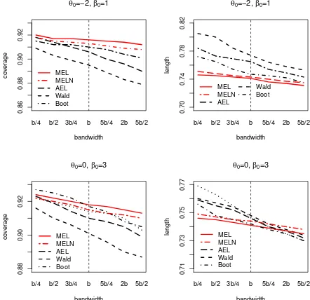
based on the pathwise derivative (MEL) and on its numerical approximation (MELN) are clearly less sensitive to the choice of the bandwidth than the other competing statistics. To further support this result, Figure 2 reports the sensitivity to different bandwidths of the finite sample coverage and av-erage length of the confidence intervals (at the 95% nominal level) forθ0and

based on the Wald statistic (Wald), its bootstrapped version (Boot) and the same AEL, MEL and MELN statistics described above. The coverage of the confidence interval based on modified test is both more accurate and less sensitive to the bandwidth parameter, while having a shorter length than those based on alternative tests.

We also report power results. Figure 3 shows the size adjusted finite sam-ple power of the tests based on the alternative hypothesesHδ=θ0+δ with

δ_{∈ {−}1.5,₋1.4, ...,₋0.1,0,0.1, ...,1.5_}forθ0=−2 andβ0 = 1 andn= 100;

those for the other values of θ0, β0 and n = 300 are similar and hence are

not shown. The figure shows that both MEL and MELN have superior fi-nite sample power compared to all the other competing statistics, which is consistent with our theoretical results in Theorems3.3and 3.4.

0.04 0.06 0.08 0.10 0.12 bandwidth siz e

θ0=−2, β0=1

b/4 3b/4 b 5b/4 5b/2

MEL MELN AEL Wald Boot 0.04 0.06 0.08 0.10 0.12 bandwidth siz e

θ0=0, β0=3

b/4 3b/4 b 5b/4 5b/2

MEL MELN AEL Wald Boot

Fig 1. Finite sample size for MEL (solid curve), MELN (two dashed curve),AEL (long dashed curve), Wald (dashed curve) and Boot (dot dashed curve) in the ATE example for

n= 100.

0.86 0.88 0.90 0.92 bandwidth co v er age

θ0=−2, β0=1

b/4 b/2 3b/4 b 5b/4 2b 5b/2 MEL MELN AEL Wald Boot 0.70 0.74 0.78 0.82 bandwidth length

θ0=−2, β0=1

b/4 b/2 3b/4 b 5b/4 2b 5b/2 MEL MELN AEL Wald Boot 0.88 0.90 0.92 bandwidth co v er age

θ0=0, β0=3

b/4 b/2 3b/4 b 5b/4 2b 5b/2 MEL MELN AEL Wald Boot 0.71 0.73 0.75 0.77 bandwidth length

b/4 b/2 3b/4 b 5b/4 2b 5b/2 θ0=0, β0=3

MEL MELN AEL Wald Boot

−1.5 −1.0 −0.5 0.0 0.5 1.0 1.5

0.0

0.2

0.4

0.6

0.8

1.0

δ

P

o

w

er

MEL MELN AEL Wald Boot

θ=−2+δ, β0=1

Fig 3. Finite sample power for MEL (solid curve), MELN (two dashed curve), AEL (long dashed curve), Wald (dashed curve), and Boot (dot dashed curve) in the ATE example for

n= 100.

that are always observed are X = (Y, X1)′, while the missing variable is W = X2 with probability of missingness (the propensity score) given by

logit(P_{(X2 is missing)) = 0.5−X1−2Y (corresponding to approximately}

30% of missing covariates). In the simulations the sample sizes aren= 100 and n= 300, and q0(·) andp0(·) are estimated with a leave-one-out kernel

estimator with bandwidths chosen using least squares cross-validation. The statistics we consider are the adjusted EL ratio (AEL), a bootstrap version of it (AELboot), the modified EL ratio based on the pathwise derivative (MEL), a Wald statistic based on (4.2) (Wald), and the modified EL ra-tio based the analytical approximara-tion (B.7) in Appendix B in the Sup-plementary Material (MELN) withV(Z, θ0) = (Ds(X, W, θ0), D), and the

analytical derivative

(5.2) bδi =

1

n

n X

j=1

1−Dj b

p(Xj)

Si− b

q(Xj) b

p(Xj)

DiKb(Xj−Xi)

,

whereSi =s(Xi, Wi, θ0).

The adjusted EL ratio is based on the feasible version of (4.2), namely

e

adjustment isρ_b=tr(Σb−1Qb)/tr(Vb−1Qb), where

b

Σ = 1

n n X i=1 b

σ2(Xi) b

p(Xi)

+_bqXi,θb

b

qXi,θb

′

,

b

σ2(x) = 1

n

Pn

i=1Dis(Xi, Wi,θb)s(Xi, Wi,bθ)′Kb(Xi−x)

n−1Pn

i=1DiKb(Xi−x) −b

q(x,θb)q_b(x,θb)′

b

V = 1

n

n X

i=1

e

s(Zi,θb)es(Zi,bθ)′, Qb=

1 n n X i=1 e

s(Zi,θb)

! _n

X

i=1

e

s(Zi,θb) !′

,

and _bq(x, θ) and p_b(x) are defined in (4.3). Then, it can be shown that

−2ρ_blogELn(θ0,bh)→d χ23. The bootstrap version of the EL ratio follows the

procedure suggested by [65] for imputed (survey) data: (1) for Di = 1 a

re-sample_{Z_i∗_}n

i=1from{Zi}ni=1and forDi = 0 a resample{bq∗(Xi∗, θ)/pb∗(Xi∗)}ni=1

from the imputed values {bq(Xi, θ)/pb(Xi)}n_i=1 are drawn to form the

boot-strap analogue _es∗(Z_i∗, θ) of _es(Zi, θ) ; (2) the bootstrap EL ratio statistic

EL∗_n(θ0,bh∗) is computed using the centered version ofes∗(Zi∗, θ0) ; (3) steps

(1)-(2) are repeated B times. The consistency of this bootstrap procedure follows by standard arguments (see for example those used by [74]). Finally, the Wald statistic is

W =nθb−θ0′ 1 n

n X

i=1

∂_es(Zi,θb)

∂θ′

! b

Σ−1 1

n

n X

i=1

∂_es(Zi,θb)

∂θ′

!′

b

θ−θ0,

where bθ is the maximum empirical likelihood estimator as defined in [74] (for exactly identified estimating equations).

The tables and figures below are based on 1000 replications. Tables 3 and 4 report, respectively, the finite sample size (at the 5% and 10% significance level) of the tests H0 : θ1 = θ10 and H0 :θ2 = θ20 and of the test for the

joint hypothesis H0 :θ1=θ10, θ2 =θ20.

n= 100 n= 300

θ1 θ2 θ1 θ2

AEL 0.090 0.123 0.085 0.118 0.075 0.112 0.071 0.111 AELboot 0.059 0.109 0.058 0.107 0.055 0.103 0.056 0.102 MEL 0.057 0.108 0.057 0.106 0.054 0.103 0.054 0.102 MELN 0.058 0.109 0.059 0.108 0.055 0.105 0.055 0.104 Wald 0.104 0.148 0.105 0.135 0.087 0.129 0.080 0.115

Table 3

n= 100 n= 300 AEL 0.085 0.122 0.079 0.115 AELboot 0.060 0.115 0.057 0.106 MEL 0.056 0.108 0.052 0.103 MELN 0.059 0.110 0.055 0.107 Wald 0.106 0.140 0.092 0.119

Table 4

Finite sample size (5%left column, 10%right column) for joint test for (θ1, θ2)in the missing data example.

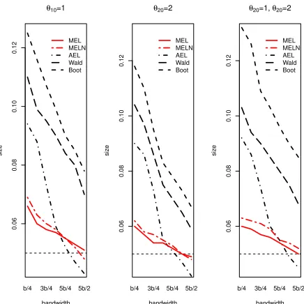
Figure 4 shows the sensitivity of the finite sample size of the testsH0 : θ1 =θ10,H0:θ2 =θ20and H0:θ1 =θ10, θ2 =θ20 to the bandwidth choice,

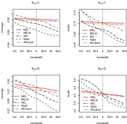
using the following values: b/4, b/2, 3b/4, 5b/4, 2b where b is the cross-validated bandwidth. Figure 5 shows the sensitivity of the finite sample coverage and average length of the confidence intervals (at the 95% nominal level) for the unknown slopesθ10and θ20 to the bandwidth choice using the

same values as those used for the finite sample size.

0.06

0.08

0.10

0.12

bandwidth

siz

e

θ10=1

b/4 3b/4 5b/4 5b/2 MEL MELN AEL Wald Boot

0.06

0.08

0.10

0.12

bandwidth

siz

e

θ20=2

b/4 3b/4 5b/4 5b/2 MEL MELN AEL Wald Boot

0.06

0.08

0.10

0.12

bandwidth

siz

e

θ20=1, θ20=2

b/4 3b/4 5b/4 5b/2 MEL MELN AEL Wald Boot

Fig 4. Finite sample size for MEL (solid curve), MELN (two dashed curve), AEL (long dashed curve), Wald (dashed curve) and AELboot (dot dashed curve) in the missing data example forn= 100.

Figure 6 shows the size adjusted finite sample power of the test based on the alternative hypothesesHδ =θ10+δforδ∈ {−1,−0.9, ...,−0.1,0,0.1, ...,1}

forθ10= 1 andn= 100 - those for the other values ofθ10, θ20andn= 300 are

0.84

0.88

0.92

bandwidth

co

v

er

age

θ10=1,

b/4 b/2 3b/4 b 5b/4 2b 5b/2 MEL

MELN AEL Wald AELboot

2.00

2.05

2.10

2.15

bandwidth

length

θ10=1,

b/4 b/2 3b/4 b 5b/4 2b 5b/2 MEL

MELN AEL Wald AELBoot

0.87

0.89

0.91

0.93

bandwidth

co

v

er

age

θ20=2,

b/4 b/2 3b/4 b 5b/4 2b 5b/2 MEL

MELN AEL Wald AELboot

3.6

3.8

4.0

4.2

4.4

bandwidth

length

θ20=2,

b/4 b/2 3b/4 b 5b/4 2b 5b/2 MEL

MELN AEL Wald AELBoot

Fig 5. Finite sample coverage at 95% (left) and average length (right) for MEL (solid curve), MELN (two dashed curve), AEL (long dashed curve), Wald (dashed curve) and AELboot (dot dashed curve) in the missing data example forn= 100.

finite sample power curves for the test ofHδ=θ1 =θ10+δ1, θ2=θ20+δ2over

the grid (δ1, δ2)∈ {−1,−0.75, ...,0, ...,0.75,1} × {−1,−0.75, ...,0, ...,0.75,1}

at the contour level of 0.4. Smaller contour plots indicate higher finite sample power.

Tables 3-4 and Figures 4-6 confirm and strengthen the results of the ATE example, as they indicate that the modified EL proposed in this paper yields test statistics characterized by finite sample properties typically better than those based on other asymptotically equivalent test statistics. As with the ATE example, both modified EL ratios are clearly less sensitive to the band-width choice than the other competing statistics and more powerful, con-firming the theoretical results of Theorems 3.3and 3.4.

−1.0 0.0 0.5 1.0

0.0

0.2

0.4

0.6

0.8

1.0

δ

P

o

w

er

MEL MELN AEL Wald AELBoot

θ₁=1+δ

δ δ 0.4

0.0 0.2 0.4 0.6 0.8 1.0

0.0

0.2

0.4

0.6

0.8

1.0

MEL MELN AEL S AELBoot

θ₁=1+δ,θ₂=1+δ

0.4

0.4 0.4 0.4

Fig 6. Finite power (left panel) and finite power contour (right panel) for MEL (solid curve), MELN (two dashed curve), AEL (long dashed curve), Wald (dashed curve) and AELboot (dot dashed curve) in the missing data example forn= 100.

Therefore, it is expected that the way the nuisance parameters are estimated (through e.g. the way a bandwidth parameter is chosen) does not have a ma-jor impact on the behavior of the modified empirical likelihood statistic. This might be particularly appealing in situations where first-steps are hard to estimate precisely (such as in high-dimensional settings). Additionally, the proposed modified EL test is efficient (in a Maximin and semiparametric sense). These theoretical results are confirmed by finite sample simulations, which further show that the new method performs favorably compared to competitors.

The ideas of this article can be extended to the problem of estimation of

θ0. An EL estimator based on the modified moments is expected to posses good bias properties, see [53] for linear functionals of densities. [19] have recently investigated the properties of related estimators in a generalized method of moments framework, allowing for machine learning methods as first-steps by virtue of the modified moment functions.

7. Proofs of the Main Results.

cor-respond to our Assumption A(v). We check their condition (A1), which corresponds to (2.7). By Assumption A, and the standard Central Limit Theorem, 1 √ n n X i=1

mZi, θ0,bh

= √1

n

n X

i=1

m(Zi, θ0, h0) +oP(1) d

→N(0,Σ).

This verifies their assumption (A1) with U =d N(0,Σ), where = stands ford equality in distribution. Finally, their assumption (A2) (which corresponds to (2.8)) holds by our Assumption A(iv) and the consistency of bh.

Proof of Theorem3.3.We follow a similar proof strategy as in Theorem

3.1. By Assumption A, under the local alternativesH1n,

1 √ n n X i=1

mZi, θ0,bh

= √1

n

n X

i=1

m(Zi, θ0, h0) +oP(1).

By Assumption C, and withθn=θ0+τ /√n,

1 √ n n X i=1

m(Zi, θ0, h0)

= √1

n

n X

i=1

m(Zi, θn, h0) +√1

n

n X

i=1

[m(Zi, θ0, h0)−m(Zi, θn, h0)]

= √1

n

n X

i=1

m(Zi, θn, h0) +√nP[m(Zi, θ0, h0)−m(Zi, θn, h0)] +oP(1)

= √1

n

n X

i=1

m(Zi, θn, h0)−G0τ +oP(1).

DefineXin =m(Zi, θn, h0).We check the conditions of Lyapounov’s Central

Limit Theorem. Note{Xin}n_i=1 are iid, with zero mean,

lim

n→∞E

XinXin′

=E_{m(Z, θ0, h0)m}′_{(Z, θ0, h0)<∞,}

and

lim

n→∞

Eh_|Xin|2+δi

nδ/2 = 0,

by Assumption C(iii). This verifies A1 in [32] withU =d N(−G0τ,Σ).Thus, by Assumption A and Theorem 2.1 in [32], under the local alternativesH1n,

where Z =d N(−Σ−1/2G0τ, I). This allows us to apply existing Maximin

theory, see [67].

Proof of Theorem 3.4. From the proof of Theorem3.3, we obtain

−2 logM ELn(θ0,bh) =Tn′Tn+oP(1),

where

Tn= √1

n

n X

i=1

−Σ−1/2m(Zi, θ0, h0).

By Corollary 3 in [20] the optimality will follow if we prove Tn=ξn(h0) + oP(1),whereξn(h0) := (nB∗)−1/2P_in₌₁S_θ∗(Zi, h0), S_θ∗(Zi, h0) is the so-called

efficient score and B∗ := V ar(S_θ∗) the efficient information, see [20] for details. By Lemma 1 in [2], see page 940 (A.33),

S_θ∗=₋G′₀Σ−1m.

Hence, B∗ = G′₀Σ−1G0 and B∗−1/2Sθ∗ = − G′0Σ−1/2

−1

G′₀Σ−1m

=₋Σ−1/2m. Thus,Tn=ξn(h0) +oP(1) and the optimality follows.

Acknowledgements. We are grateful to the Co-Editor, the Associate Editor and referees for suggestions that have improved our paper.

SUPPLEMENT