Three-dimensional doubly diffusive convectons: instability and transition to complex dynamics

This is a repository copy of

Three-dimensional doubly diffusive convectons: instability and

transition to complex dynamics

.

White Rose Research Online URL for this paper:

http://eprints.whiterose.ac.uk/125239/

Version: Accepted Version

Article:

Beaume, C, Bergeon, A and Knobloch, E (2018) Three-dimensional doubly diffusive

convectons: instability and transition to complex dynamics. Journal of Fluid Mechanics,

840. pp. 74-105. ISSN 0022-1120

https://doi.org/10.1017/jfm.2017.905

© Cambridge University Press 2018. This is an author produced version of a paper

published in Journal of Fluid Mechanics. Uploaded in accordance with the publisher's

self-archiving policy.

[email protected] https://eprints.whiterose.ac.uk/ Reuse

Items deposited in White Rose Research Online are protected by copyright, with all rights reserved unless indicated otherwise. They may be downloaded and/or printed for private study, or other acts as permitted by national copyright laws. The publisher or other rights holders may allow further reproduction and re-use of the full text version. This is indicated by the licence information on the White Rose Research Online record for the item.

Takedown

If you consider content in White Rose Research Online to be in breach of UK law, please notify us by

Three-dimensional doubly diffusive

convectons: instability and transition to

complex dynamics

C´

edric Beaume

†

, Alain Bergeon

and Edgar Knobloch

1_{School of Mathematics, University of Leeds, Leeds LS2 9JT, UK} 2

Institut de M´ecanique des Fluides de Toulouse (IMFT), Universit´e de Toulouse, CNRS, INPT, UPS, Toulouse, France

3

Department of Physics, University of California, Berkeley CA94720, USA

(Received xx; revised xx; accepted xx)

Three-dimensional doubly diffusive convection in a closed vertically extended container driven by competing horizontal temperature and concentration gradients is studied by a combination of direct numerical simulation and linear stability analysis. No-slip boundary conditions are imposed on all six container walls. The buoyancy numberN is taken to be−1 to ensure the presence of a conduction state. The primary instability is subcritical and generates two families of spatially localised steady states known as convectons. The convectons bifurcate directly from the conduction state and are organized in a pair of primary branches that snake within a well-defined range of Rayleigh numbers as the convectons grow in length. Secondary instabilities generating twist result in secondary snaking branches of twisted convectons. These destabilize the primary convectons and are responsible for the absence of stable steady states, localized or otherwise, in the subcritical regime. Thus all initial conditions in this regime collapse to the conduction state. As a result, once the Rayleigh number for the primary instability of the conduction state is exceeded, the system exhibits an abrupt transition to large amplitude relaxation oscillations resembling bursts with no hysteresis. These numerical results are confirmed here by determining the stability properties of both convecton types as well as the domain-filling states. The number of unstable modes of both primary and secondary convectons of different lengths follows a pattern that allows the prediction of their stability properties based on their length alone. The instability of the convectons also results in a dramatic change in the dynamics of the system outside the snaking region that arises when the twist instability operates on a time scale faster than the time scale on which new rolls are nucleated. The results obtained are expected to be applicable in various pattern-forming systems exhibiting localized structures, including convection and shear flows.

Key words: Authors should not enter keywords on the manuscript, as these must be chosen by the author during the online submission process and will then be added during the typesetting process (see http://journals.cambridge.org/data/relatedlink/jfm-keywords.pdf for the full list)

1. Introduction

Spatially localised states, both stationary and travelling, are commonly found in fluid flows, notably in convection and shear flows. In this work we are interested in localised states consisting of a segment of a periodic state embedded in a homogeneous background state, corresponding either to a conduction state or to laminar shear flow. Much useful and transferable information about states of this type can be gleaned from studies of the bistable Swift–Hohenberg equation in one spatial dimension with periodic boundary conditions and left-right symmetry (Burke & Knobloch 2006). In particular, it is known that in a periodic domain with a finite but large period, localised states bifurcate from the primary branch of subcritical spatially periodic states and that they do so already at small amplitude, i.e., close to the primary bifurcation. This bifurcation is likewise subcritical and in the simplest case generates a pair of unstable localised states with reflection symmetry. However, with decreasing forcing these states acquire stability via folds and thereafter the two branches of localised states oscillate between a pair of well-defined limits in parameter space in a behaviour known as homoclinic snaking (Woods & Champneys 1999). During each back and forth oscillation the localised state grows in length via the nucleation of a new wavelength on either side. As one follows the branches upward each gains stability at a left fold and loses stability at a right fold, thereby generating a large multiplicity of simultaneously stable localised states of different lengths within the snaking region. The wavelength of the structure embedded in the background homogeneous state depends on the location in the snaking region and increases along the stable branch segments from left to right. Close to the folds of the snaking branches, additional bifurcations occur that produce asymmetric spatially localised states. These states, known asrung states, are always unstable and lie on branches that interconnect the intertwined branches of symmetric localised states forming a snakes-and-ladders

structure (Burke & Knobloch 2006, 2007a,b). Related behaviour is present in systems with midplane reflection symmetry (Burke & Knobloch 2007b) and in structures localised in two spatial dimensions (Avitabileet al.2010).

Spatially localised states are also found in a large variety of other fluid systems, ranging from ferrofluids (Lloydet al.2015) to colloidal suspensions (Lioubashevskiet al.

1999), and display strikingly similar properties. Historically, localised states in fluids were first identified in doubly diffusive convection, a term describing convection in a binary fluid mixture driven by imposed temperature and concentration differences. The first such states, now referred to as convectons, were computed in 1997 in natural doubly diffusive convection in a two-dimensional vertically extended cavity, i.e., convection driven by horizontal gradients (Ghorayeb & Mojtabi 1997) but their snaking structure was discovered only a decade later (Bergeon & Knobloch 2008b). Parallel studies of localised doubly diffusive convection in two-dimensional horizontally extended domains (Batiste et al. 2006; Mercader et al. 2009; Beaume et al. 2011; Mercader et al. 2011; Watanabeet al.2012, 2016) have established a solid relationship between these types of problems and the phenomenology captured so effectively by the bistable Swift–Hohenberg equation. In shear flows localised states also snake (Schneider et al. 2010a; Gibson & Schneider 2016) and moreover may lie on the separatrix between laminar and turbulent flows (Duguet et al. 2009; Schneideret al. 2010b) and so play a prominent role in the transition to turbulence. An ever-increasing catalogue of localised states in shear flow is now available (Avila et al.2013; Khapkoet al. 2013; Brand & Gibson 2014; Gibson & Brand 2014; Mellibovsky & Meseguer 2015).

snaking region such solutions will grow in length dynamically, resulting in the invasion of the background conduction state by stable convection. This is in fact the case in both two-dimensional natural doubly-diffusive convection (Bergeon & Knobloch 2008b) and in two-dimensional binary fluid convection in a horizontal layer (Batiste et al. 2006). However, this attractive picture of the dynamics does not extend to three dimensions. Already in 2002 Bergeon and Knobloch showed that in three dimensions the large amplitude domain-filling state is unstable (Bergeon & Knobloch 2002). As a result a subcritical steady state primary instability does not generate a hysteretic transition to large amplitude stationary convection but results instead in a nonhysteretic transition to a finite-amplitude relaxation oscillation. This remarkable behaviour extends to three-dimensional natural doubly diffusive convection in vertically extended domains (Beaume

et al. 2013a). In particular, an analogous instability, now responsible for the presence of unstable twisted convectons, destabilizes the quasi two-dimensional convectons re-sembling those computed by Bergeon & Knobloch (2008b). The consequences of this instability are similar and dramatic: the large amplitude stationary domain-filling state is destabilized, and convectons both within and above the snaking region collapse to the conduction state instead of evolving to the large amplitude state (Beaumeet al.2013a). This unexpected behaviour motivates the present work. Specifically, we wish to confirm the results of earlier direct numerical simulations of three-dimensional natural doubly diffusive convection by performing explicit linear stability calculations for both the quasi two-dimensional convectons computed by Bergeon & Knobloch (2008b) and the fully three-dimensional twisted convectons computed by Beaumeet al. (2013a). In fact, only Watanabe et al. (2016) have thus far investigated the detailed stability properties of localised states in a fluid flow, and this in the context of two-dimensional binary fluid convection in a horizontal layer with a negative Soret effect. The present work extends this type of analysis to three dimensions and provides an exhaustive account of the stability properties of convectons in three-dimensional natural doubly diffusive convection. The results confirm those obtained in direct numerical simulations and provide a guide to understanding the complex dynamics displayed by the present system near threshold for the primary instability of the conduction state.

In the following section, we introduce the specific case of natural doubly diffusive convection that we study and summarize the state of the art. Section 3 provides an ex-haustive account of the stability properties of each of the various convecton types known to be present in this system and describes the results of direct numerical simulations of the system in the vicinity of the snaking region. The paper concludes with a summary and discussion of the results obtained.

2. Problem set-up

2.1. Doubly diffusive convection

Following Beaumeet al. (2013a) we consider doubly diffusive convection in a binary fluid placed within a three-dimensional box of square cross-section in the horizontal and large extent in the vertical. We use the coordinatexfor the vertical direction and (y, z) for the horizontal coordinates. Convection is produced by competing but balanced horizontal gradients of temperature and concentration that result from the imposition of appropriate Dirichlet boundary conditions atz= 0, l leading to the conduction state u∗ = 0,T∗

=Tr+z△T /l,C∗ =Cr+z△C/l, whereT∗ is the temperature, C∗ is the

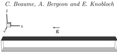
Figure 1.Sketch of the physical domain from an angle similar to that used in subsequent figures. For convenience the system has been rotated clockwise by 90◦

. As a result, the acceleration due to gravity points towards the left. Shaded boundaries are maintained at fixed temperature and concentration with the darker wall maintained at higher values ofT andCthan the lighter one. Only a portion of the domain inxis shown.

△C >0 are the imposed temperature and concentration differences across the box. We nondimensionalize the governing equations usingl for lengths,△T for the temperature,

△C for the concentration and l2

/κ for the time, where κis the thermal diffusivity. In absence of cross-diffusion, the Boussinesq equations describing the system are

P r−1_[∂

tu+ (u· ∇)u] =−∇p+Ra(T −C)ˆx+∇2u, (2.1)

∇ ·u= 0, (2.2)

∂tT + (u· ∇)T =∇2T, (2.3)

∂tC+ (u· ∇)C=τ∇2C. (2.4)

Here u = (u, v, w) is the dimensionless velocity field in (x, y, z) coordinates, p is the dimensionless pressure, T ≡(T∗_−T

r)/△T is the dimensionless temperature andC ≡

(C∗ _−C

r)/△C is the dimensionless concentration. The above equations involve three

dimensionless numbers: the Rayleigh numberRa≡g|ρT|△T l3/ρ0νκ, the Prandtl number P r ≡ν/κ and the (inverse) Lewis numberτ≡D/κ, whereg is the gravitational accel-eration,ρT/ρ0<0 is the thermal expansion coefficient in the Boussinesq approximation

evaluated atTr,ρ0 is the density of the fluid atTr, andν andD are, respectively, the

kinematic viscosity and the molecular diffusivity of the heavier fluid component, both assumed to be constant. In writing this set of equations, we have assumed that the buoyancy ratioN ≡ρC△C/ρT△T =−1. With this choice of N the system (2.1)–(2.4)

possesses the stationary conduction solution alluded to above.

The physical domain is a closed container of square horizontal cross-section and aspect ratio L ≫ 1 in the vertical direction, as shown in figure 1. We prescribe no-slip boundary conditions for the velocity everywhere and no-flux boundary conditions for the temperature and concentration on all walls exceptz= 0,1:

x= 0, L:u=v=w=∂xT =∂xC= 0, (2.5)

y= 0,1 :u=v=w=∂yT =∂yC= 0, (2.6)

z= 0 : u=v=w=T =C= 0, (2.7)

z= 1 : u=v=w=T−1 =C−1 = 0. (2.8) The system (2.1)–(2.4), together with the boundary conditions (2.5)–(2.8), admits the conduction solution (u, v, w, T, C) = (0,0,0, z, z) for all values of the parameters Ra,

P r and τ. In terms of the perturbation quantities (u, v, w, Θ, Σ) with Θ ≡ T −z and

Σ ≡C−z, the system is equivariant with respect to the dihedral groupD2 generated

by the two reflections

Sy: [u, v, w, Θ, Σ](x, y, z)−→[u,−v, w, Θ, Σ](x,1−y, z), (2.9)

The group structure implies that the equations are also equivariant with respect to

Sc=Sy◦S△:

Sc: [u, v, w, Θ, Σ](x, y, z)−→ −[u, v, w, Θ, Σ](L−x,1−y,1−z). (2.11)

These symmetries play a key role in the properties of the solutions described below. In particular, the symmetryS△plays a role that is analogous to the role played by spatial

reflection symmetry in the Swift–Hohenberg equation.

WhenN 6=−1 the properties of the system change dramatically. In particular, there is no motionless conduction state and the base state now consists of a single large scale roll that spans the whole domain 06x6L. This circulation is responsible for changing the primary bifurcation to an imperfect bifurcation for values ofN close to −1. Additional effects can be identified forN farther away from−1. In this paper we focus on the case

N =−1 only.

We solve the system (2.1)–(2.4) numerically using a splitting scheme for time evolution and a finely tuned numerical continuation algorithm (Beaume 2017). Throughout this paper, the parameters are chosen following (Xinet al.1998; Bergeon & Knobloch 2002):

P r = 1,τ = 1/11 and L= 19.8536, corresponding to eight wavelengths of the primary instability of the two-dimensional problem. The Rayleigh numberRais kept as a control parameter.

2.2. State of the art

Spatially localised solutions of doubly diffusive convection in a vertically extended domain have been studied for over 10 years. Their origin was first investigated in a study of near-onset behaviour in a two-dimensional vertically periodic slot of relatively small spatial period (Bergeon & Knobloch 2008a). These authors found a number of spatially periodic states yielding a complex bifurcation diagram and identified states composed of a single roll occupying a part of the domain. This study was followed up by a study describing the evolution of spatially localised doubly diffusive convectons in the same configuration but with a large spatial period in the vertical (Bergeon & Knobloch 2008b). The authors showed that the primary bifurcation from the conduction state is subcritical. The resulting spatially periodic solution is S△-symmetric and transforms rapidly into

an array of corotating rolls as one proceeds away from the primary bifurcation, before turning towards larger values ofRaat a fold and generating an array of large amplitude corotating rolls. During this process the solution remains S△-symmetric. Subsequent

branches of spatially periodic states with different wavenumbers but alsoS△ symmetry

behave in the same way but may acquire stability at large amplitude. As expected from earlier studies of the Swift–Hohenberg equation, the primary subcritical branch of spatially periodic states becomes unstable almost immediately to spatially modulated states – still S△-symmetric – and these evolve rapidly with decreasingRa into strongly

localised states exhibiting homoclinic snaking (Woods & Champneys 1999; Burke & Knobloch 2006). As in the Swift–Hohenberg equation there are two branches of localized states, one consisting of an odd number of corotating rolls all rotating clockwise about the y axis and the other of an even number of corotating rolls also rotating clockwise. In the following we refer to these states as L+ _{and L}−_{, respectively, and emphasize}

that each isS△-symmetric with respect to the center of the domain. In contrast to the

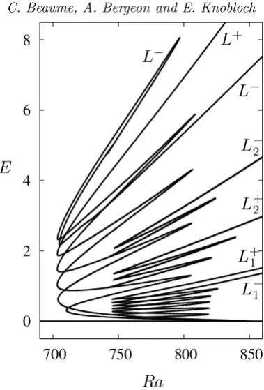
Figure 2. Bifurcation diagram representing the total kinetic energy E as a function of the Rayleigh numberRa. The solutionE = 0 corresponds to the conduction state and convectons (E >0) emerge through a sequence of bifurcations from the conduction state atRa≈850.86. The primary branchesL±consist of corotating rolls with axes parallel to theyaxis. Solutions on the secondary branchesL+

1,L + 2 andL

−

1,L

−

2 bifurcate fromL

±

and break the symmetrySy. Such states are referred to astwisted.

in related systems, however, confirming the basic bifurcation scenario (Mercader et al.

2013; Lo Jaconoet al.2017).

The above properties of the system persist in two-dimensional domains with endwalls at x = 0, L. However, such walls destroy the translation invariance of the system in thexdirection and prevent the formation of spatially periodic solutions (Beaumeet al.

2013a). As a result localised states bifurcate directly from the conduction state (Mercader

et al.2009) rather than appearing in a secondary bifurcation from a periodic state. This behaviour persists in three-dimensional domains with no-slip walls (Sezai & Mohamad 2000; Bergeon & Knobloch 2002). In this case all the primary branches have an additional symmetry, the reflection symmetrySy. This symmetry exerts a substantial influence on

the properties of the resulting solutions since it can be broken in secondary bifurcations, a fact responsible for the formation of twisted localised states (Beaumeet al.2013a), as discussed further below.

The bifurcation diagram for steady doubly diffusive convectons in a three-dimensional domain of square cross-section and aspect ratio L= 19.8536 is shown in figure 2. The solutions are represented in terms of the total kinetic energy:

E=1 2

Z 1

0

Z 1

0

Z L

0

(u2

+v2

+w2

(a) (b)

L+ L−

Figure 3.Convectons with the lowest kinetic energy along the branchL+

atRa= 710.4464 (a) andL−

atRa= 703.9686 (b) represented in terms of the isocontoursu=±0.3. Positive values are shown in red. In this and subsequent figurese_{xpoints to the right (gravitational acceleration} is to the left) ande_{z points upward.}

convectons,L+ _andL−

, both of which snake within the interval 703.Ra.807. Both types of convectons are fully symmetric, i.e., invariant underSy, S△and, by extension, Sc. Convectons from the branch L+ possess an odd number of corotating, clockwise

rolls centered in the domain while those from the branchL−

possess an even number of corotating, clockwise rolls also centered (see figure 3). These states differ from those found in a two-dimensional periodic domain in minor ways only: (i) because the boundary conditions at x= 0, Lare no longer periodic, no spatially periodic state is present and the convectons therefore cannot and do not connect to any spatially periodic state, and (ii) owing to the no-slip boundary condition iny, the convecton structure is fully dimensional. Despite these differences, the snaking in the two-dimensional and three-dimensional systems is similar: in the direction of increasing energy, going from a left fold to the next right fold (hereafter called a positive segment, alluding to the fact that

Ra increases), the corotating rolls strengthen, while going from a right fold to the next left fold (hereafter called a negative segment –Radecreases) results in the nucleation of one new roll on either side of the roll structure.

Secondary bifurcations occur along the negative segments of these snaking branches. These symmetry-breaking bifurcations all break the Sy symmetry together with one

other reflection and yield roll structures we refer to astwisted. In these states the axes of adjacent rolls are rotated in opposite directions around the vertical axis. One such pitchfork bifurcation occurs along the first negative segment ofL+ _{(counting from low}

to high energy) and yields the branchL+

1 of twisted convectons, while two bifurcations

occur in very close succession along the first negative segment ofL−

. One of these yields the branchL−1 shown in figure 2 but we have not been able to continue the states created

in the other. The states on theL+1 branch near its birth consist of a singleSc-symmetric

roll, i.e., a roll whose axis is rotated about the vertical, while theL−1 branch consists of

two-rollS△-symmetric states rotated in opposite directions about this axis. These states

are shown in figure 4(a,b).

Successive secondary bifurcations yielding both Sc- and S△-symmetric twisted

con-vectons can be found alongeach subsequent negative segment of each primary branch. We refer to the Sc-symmetric states bifurcating from the second negative segment of

the L+ _{branch as L}+

2c and to the S△-symmetric states bifurcating from this segment

as L+

2△. These branches are indistinguishable in the bifurcation diagram in figure 2 and

are therefore labeledL+

2 for simplicity. Both consist of solutions composed of one broad

untwisted roll inherited from theL+_{branch, surrounded by two narrower rolls of smaller}

amplitude and rotated about thexaxis, as shown in figure 4(c,d). This figure also shows solutions L−

2c and L −

2△ produced in successive bifurcations along the second negative

segment ofL−

(a) (b) (c) (d) (e) (f)

L+ 1 L−

1 L+

2c

L+ 2_△ L−

2c

L− 2_△

Figure 4.Convectons with the lowest kinetic energy along the branch L+1 at Ra= 817.9884

(a), L−1 at Ra = 818.0300 (b),L +

2c at Ra = 820.0688 (c), L

+

2△ atRa = 820.1873 (d),L −

2c at

Ra= 823.9576 (e) andL−2△ atRa= 823.4842 (f) represented in the same way as in figure 3.

right fold, each structure gradually nucleates a pair of new rolls, one on either side, with rotation that is always opposite to that of the roll adjacent to it.

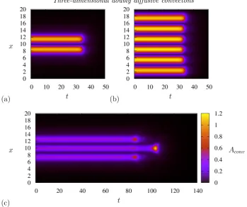
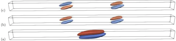
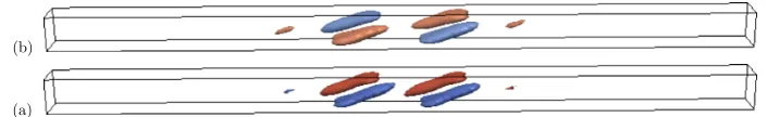
Having recapitulated existing results we now present three examples of the evolution of the system initialized with the three-dimensional states just described. In figure 5(a) we present the temporal evolution of a quasi two-dimensional localized L− _convecton,

followed in figure 5(b) by that of an initial condition taken from the same branch but that is domain-filling and in figure 5(c) by that of a secondary twisted convecton from theL+

1 branch. The time evolution is represented in terms of the convection amplitude

quantified through the quantity

Aconv=

s Z 1

0

Z 1

0

u2_{dy dz (2.13)}

This measure of convection strength is appropriate since u is the dominant velocity component. The interesting and remarkable fact is that all our initial conditions ulti-mately collapse to the conduction state, whether they are very localized, domain-filling or twisted. This observation suggests that all the nontrivial states in the subcritical regime of this problem are unstable. The main goal of this paper is to explain this remarkable fact and explore its consequences.

3. Convecton stability

In this section, we report on the stability properties of the primary convectons L±

together with those of the twisted convectons L±

iS, with i = 1,2 and S = c,△. Our

results describe the evolution of all unstable eigenmodes along the snaking branches and the stability of a given convecton is hereafter reported in terms of a pair of integers (Nr, Ni), whereNrrepresents the number of real unstable eigenvalues andNithe number

of pairs of unstable complex conjugate ones. Eigenmodes with a real unstable eigenvalue correspond to instabilities with monotonic growth while those with a complex pair of unstable eigenvalues correspond to instabilities with oscillatory growth.

Figure 5. Space-time evolution of three subcritical states: (a) L− convecton obtained at

Ra ≈ 747.14104 and time-integrated at Ra = 747.1410, (b) L− convecton obtained at

Ra ≈ 756.04067 and time-integrated at Ra = 756.0407 and (c) L+1 convecton obtained at Ra≈775.76716 and time-integrated atRa= 775.7672.

For this purpose we perturb the stationary solutionsF(x) in the following way:

f(x, t) =F(x) +ǫRe{˜f(x)eλt}, (3.1) where ǫ is a small real parameter and˜f(x) is the eigenfunction corresponding to the complex temporal growth rateλ≡λr+iλi. We refer toλras the growth rate andλi as

the frequency of the mode and present the growth rate results in terms of the quantity

eλr. Eigenvaluesλ

r such that eλr >1 (resp. < 1) are associated with unstable (resp. stable) eigenmodes.

It is important to emphasize here that the bifurcation generating the convectons is in fact the second primary bifurcation (Beaumeet al.2013a). The first instability takes place at Ra ≈ 850.78, i.e., slightly earlier than the transcritical bifurcation at Ra ≈850.86. This bifurcation breaks the symmetryS△but respectsSy (the corresponding eigenmode

is shown in figure 6(a)) and so is a pitchfork. However, this bifurcation is expected to be subcritical (Bergeon & Knobloch 2002), a fact confirmed here by direct numerical simulations (not shown), and hence does not lead to stable small amplitudes states. However, the presence of this bifurcation is key in one important respect: the resulting weakly unstable eigenvalue is inherited by both convecton branches, and as shown below, plays a significant role in their dynamics. The next mode that becomes unstable is an even mode that breaks no symmetry (figure 6(b)), and the corresponding bifurcation, atRa≈850.86, is therefore transcritical. This bifurcation generates the branches L±

(a) (b)

Figure 6. (a) Odd eigenmode responsible for the pitchfork bifurcation at Ra ≈ 850.78. (b) Even eigenmode responsible for the transcritical bifurcation atRa≈850.86. Both eigenmodes are computed atRa= 850.8 and represented using the two isocontours ˜u=±0.5 max(|u˜|).

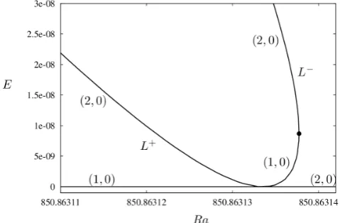
Figure 7.Enlargement of the vicinity of the primary transcritical bifurcation atRa≈850.86 producing the convecton branchesL+

andL−

in figure 2. Note how close the saddle-node (full circle) onL−is to the primary bifurcation both in terms of the kinetic energyEand the Rayleigh numberRa. Stability is indicated in terms of the notation (Nr, Ni) introduced in the text.

evolves into the convecton branch L+ _{while the supercritical branch evolves into the}

convecton branch L−

; the latter undergoes a fold at very small amplitude at which it turns towards smaller values of Ra. These small amplitude results are summarized in figure 7.

The alternation between symmetry-breaking and symmetry-preserving bifurcation is a standard feature of symmetric bifurcation problems (Hirschberg & Knobloch 1997) and is responsible for much of the weakly nonlinear behaviour observed in such systems. Here both modes are spatially modulated, a consequence of the no-slip boundary conditions at the top and bottom of the domain. The linear eigenmodes of the nonlinear states that result likewise split into odd and even families. Specifically, the since both L+

and L−

are even under appropriate reflections all eigenmodes ofL±

will have either odd or even parity.

3.1. Stability of the primary convectons

Our eigenvalue computations show that all unstable modes of the convecton branches

L± _{are associated with monotonic growth:λ}

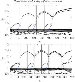
i = 0. Figure 8 shows the resulting growth

rates λr along both branches as a function of the arclength s. The L+ branch is

subcritical and is thus characterized by one unstable amplitude mode in addition to the unstable eigendirection inherited from the primary pitchfork (see table 1). The branch becomes three times unstable at s ≈ 100 (Ra ≈ 750) owing to the onset of the twist instability responsible for the secondary branchL+

1. The twist instability is triggered by

e

s

e

s

Figure 8.Linear stability results forL+ (top) andL− (bottom). The results are presented in terms of the quantityeλr

and shown as a function of the arclengths along the branch. Folds correspond to saddle-node bifurcations (λr= 0) and are denoted by vertical lines. Bifurcations generating twist are denoted by a blue dot. One weakly unstable eigenvalue (eλr

≈1) is always present.

untils≈ 100 139 236 300 337 443 503 544 800

L+ _{stability (2,0) (3,0) (2,0) (4,0) (6,0) (4,0) (6,0) (8,0) (6,0)}

untils≈ 12 108 148 252 314 351 459 525 561 650

L−

stability (2,0) (3,0) (5,0) (3,0) (5,0) (7,0) (5,0) (7,0) (9,0) (7,0)

Table 1.Stability count associated with the branchL+

(top two lines) andL−

(bottom two lines) as a function of the arclengths. The first number represents the number of unstable real eigenvalues while the second number shows the number of pairs of unstable complex conjugate of eigenvalues. The count was stopped ats= 800 forL+

ands≈650 forL−

where the branch undergoes a saddle-node induced by the finite size of the domain.

rotated around thexaxis by 90◦

as compared to that in the base state, resulting in the progressive rotation of the convection roll around thexaxis as the instability develops. At

(a) (b)

Figure 9. (a) L+ _{convecton at}

Ra ≈ 749.6782 (s ≈ 101) represented using the same color scheme as in figure 3. (b) Twist instability eigenmode for the state in (a) represented using the two isocontours ˜u=±0.5 max(|u˜|).

(a) (b)

Figure 10. (a) L+

convecton atRa ≈711.6782 (s ≈139) represented using the same color scheme as in figure 3. (b) Amplitude eigenmode for the state in (a) represented in the same way as in figure 9(b). This eigenmode is responsible for both the primary bifurcation and the first saddle-node ofL+

.

(a) (b) (c)

Figure 11. (a) L+ _{convecton at}

Ra ≈802.1785 (s ≈239) represented using the same color scheme as in figure 3. (b) Amplitude and (c) phase eigenmodes for the state in (a) represented in the same way as in figure 9(b). The former is responsible for the second and third saddle-nodes while the latter is responsible for the emergence of drifting rung states via parity-breaking bifurcations.

base convection roll. This eigenmode remains stable along the whole subsequent snaking branch as it acts only on the central roll. The next two saddle-nodes are caused by the destabilization and restabilization of a different eigenmode, shown in figure 11(b). The figure shows that this mode is responsible for the addition of one convection roll on either side of the localized structure, a process that takes place just beyond this fold (s≈236). This eigenmode becomes stabilizing at the next saddle-node (s ≈337) and remains so thereafter since it always determines the stability of the same two rolls. Consequently, each subsequent pair of saddle-nodes is generated by a new and different eigenmode. This is so for the phase mode (figure 11(c)) as well, and is in contrast to the Swift– Hohenberg equation where the same two amplitude and phase eigenvalues repeatedly pass through zero as one follows the snaking branches (Burke & Knobloch 2006; Kao

et al. 2014; Knobloch 2015). The saddle-node at s≈ 236 is followed shortly thereafter by a symmetry-breaking bifurcation triggered by a phase mode, breaking theS△andSc

symmetries but preserving theSysymmetry. This bifurcation creates a corotating roll on

(a) (b) (c)

Figure 12. (a) L+

convecton atRa ≈738.1785 (s ≈303) represented using the same color scheme as in figure 3. (b)S△-preserving twist eigenmode for the state in (a). (c)Sc-preserving twist eigenmode for the state in (a). Both eigenmodes are represented in the same way as in figure 9(b).

(a) (b)

Figure 13.(a)L−convecton atRa≈837.8913 (s≈12) represented using the same color scheme as in figure 3 but for isocontoursu=±0.1. (b) Eigenmode for the state in (a) represented in the same way as in figure 9(b).

(see below). The next change in stability is located farther away on the negative segment at s ≈ 300 (Ra ≈ 740, see Table 1) where two successive bifurcations take place in rapid succession. These bifurcations are of the same nature: they are both produced by eigenmodes breaking the symmetry Sy and one other symmetry, and result in rotation

of the axes of the end rolls either in the same or opposite direction as shown in figure 12. Since these modes act on the end rolls, their regions of influence are separated by the central roll where the eigenmode vanishes. As a result, there is little dynamical difference between them and the associated bifurcations occur at similar values ofs, equivalently

Ra. These twist modes destabilize the solution yet further. However, at the next left saddle-node (ats≈335) the amplitude and phase mode become stabilizing again, albeit at slightly different values of Ra. This scenario then repeats during each and every oscillation of theL+

branch. Overall, theL+

solution gains two unstable eigendirections during each such oscillation, as summarized in table 1.

The branchL−

emerges supercritically from the transcritical bifurcation that produces

L+_{but is initially once unstable, owing to the pitchfork bifurcation that precedes it. The}

branch undergoes a saddle-node at low amplitude as shown in figure 7 where the solution gains a second unstable eigendirection and thereafter undergoes a similar sequence of bifurcations asL+

, as summarized in Table 1. The eigenvalue count is initialized at the small amplitude saddle-node. Ats≈12 (Ra≈838), the solution gains a third unstable direction with the corresponding eigenmode shown in figure 13. The figure shows that this mode strengthens one of the endrolls comprising the solution at the expense of the other. This instability likely corresponds to the termination of the branch created in the primary pitchfork bifurcation (Bergeon & Knobloch 2002). Proceeding up the negative branch segment, one next encounters a pair of near-simultaneous bifurcations ats≈108 (Ra ≈ 742) responsible for generating the twisted states labeled L−

1 following similar

notation forL+

1 (figure 14). After this original set of bifurcations, theL

−

branch follows a similar behaviour to L+_{, gaining two unstable eigendirections during each back and}

(a) (b) (c)

Figure 14. (a) L−

convecton atRa ≈741.8996 (s ≈108) represented using the same color scheme as in figure 3. (b)S△-preserving twist eigenmode for the state in (a). (c)Sc-preserving twist eigenmode for the state in (a). Both eigenmodes are represented in the same way as in figure 9(b).

(a) (b)

Figure 15. (a) L+ _{convecton at}

Ra ≈805.7820 (s ≈440) represented using the same color scheme as in figure 3. (b) Odd parity drift eigenmode for the state in (a) represented in the same way as in figure 9(b).

(a) (b)

Figure 16.Initial condition (a) and final state (b) obtained through direct numerical simulation with imposed Sy symmetry at Ra = 757.141 (s ≈ 200). The states are represented by the isocontours|u|= 1.1.

the right fold. A pair of twist instabilities occurs along each negative segment of the branch leading to the net generation of two unstable eigendirections per back and forth oscillation.

It will have been observed that bothL+_andL−_{possess a weakly unstable eigenvalue,}

with growth rate aroundλr≈10−4for a one-roll (strongly localized) state andλr≈10−3

for a six-roll (domain-filling) state. The corresponding eigenfunction for a L+ _solution

consisting of three convection rolls is shown in figure 15(b) and is ofodd parity. In the following we use this term to refer to eigenfunctions that are odd with respect toS△, the

symmetry ofL±

, but invariant underSy. In a vertically unbounded system bifurcations

triggered by the destabilization of an odd parity mode are associated with the onset of drift and are sometimes called drift bifurcations.

To unveil the consequences of the presence of this mode, we selected a solution that allows us to suppress all other unstable eigendirections by imposing appropriate symmetry conditions on a time simulation. For this purpose we selected a solution on the second positive segment ofL− _{(counting the very small amplitude segment shown in}

figure 7) atRa≈757.1410 consisting of a pair of convection rolls. This state is shown in figure 16(a) and possesses three unstable eigendirections, two of which are associated with the twist instability and are even inx(see figure 8) and one with odd parity inx. Since the twist instability breaks the symmetry Sy while the odd parity mode does not, we

x A_conv

t

Figure 17.Space-time evolution atRa= 757.141 of the quantityAconv defined in expression

(2.13) and initialized with the state in figure 16(a).

The effect of the odd parity mode is represented in figure 17 using the quantity Aconv

defined in expression (2.13). The figure shows that drift occurs on a timescale on the order of 104

time units, a timescale that compares well with the magnitude of the odd parity mode eigenvalue. In this simulation, the convecton drifts downward until it meets the bottom wall. By symmetry, an upward drifting convecton can also be obtained. When the convecton meets the wall, it stops drifting and settles into a steady state in which the roll closest to the wall is stronger than that farther away. This wall-attached convecton has been converged using a Newton method (see figure 16(b)) and is twice unstable, each unstable eigendirection being responsible for the twist of one of the rolls. We expect that these states also snake, much like similar states in binary fluid convection in a horizontal layer (Mercaderet al.2011).

We can understand these results as follows. In an unbounded, translation-invariant system a growing odd parity perturbation would render an even state asymmetric. Since in such systems asymmetric states generically drift, the appearance of such an unstable mode is associated with a parity-breaking or drift bifurcation. In the present case, however, the walls as x= 0, L prevent translation, implying that the presence of a growing odd mode must lead to a stationary state. A simple model equation, studied by Knobloch et al. (1995) and Dangelmayr et al. (1997), captures the effect of broken translation invariance on the parity-breaking bifurcation. The model takes the form

˙

c= (µ+δcosφ−c2

)c+ηsinφ; φ˙ =c−ǫsinφ, (3.2) where µ is the bifurcation parameter and δ, η, ǫ are parameters proportional to the amplitude of the spatial inhomogeneity, assumed small and of period 2π. When these terms are absent Eq. (3.2) reduces to the normal form for the parity-breaking bifurcation, assumed here to occur atµ= 0 and to be supercritical, withc the drift speed andφthe spatial phase or displacement. Whenδ,η,ǫ are nonzeroc is no longer a drift speed but must be interpreted as the degree of asymmetry of the state. There are then generically two fixed points (c, φ) = (0,0) and (0, π), corresponding to a symmetric state at the “wall” (φ= 0) and a symmetric state at the center of the domain (φ=π), respectively. Other, asymmetric fixed points (with c 6= 0) may be present as well (Knoblochet al.

e

s

e

s

1 (top) andL

−

1 (bottom). The results are presented in

terms of the quantityeλr

and shown as a function of the arclengths along the branch. Folds correspond to saddle-node bifurcations (λr = 0) and are denoted by vertical lines. Eigenvalue collisions are indicated by a red dot.

In our case the final state that results is not symmetric but this is a consequence of the nonperiodic boundary conditions employed in the simulation.

3.2. Stability of the twisted convectons

The stability properties along the lowest branches of twisted convectons, L±

1, are

summarized in figure 18. TheSc-symmetric twisted convectons onL+1 bifurcate towards

higher Rayleigh numbers and are thus initially three times unstable: in addition to the unstable eigendirection associated with the twist instability and responsible for the formation of the branch, the L+

1 convectons are also unstable with respect to an

amplitude mode (responsible for the primary transcritical bifurcation) and a phase mode inherited from the odd parity drift mode ofL+_{. Very close to the bifurcation point to} L+

1 the amplitude eigenvalue decreases while the twist eigenvalue increases resulting in

an eigenvalue collision ats≈4.7 (Ra≈756.1) forming a complex conjugate pair. Such a collision is possible because both modes have the same symmetry and is shown in the left panel of figure 19; the imaginary part of the eigenvalues along the L+

1 branch is shown

in figure 20. The resulting (1,1) unstableL+1 convecton continues to larger values ofRa

with the unstable eigenmodes atRa≈781.9884 shown in figure 21.

eλr

s

eλr

s

Figure 19.Enlargement of thes∈[1,6] interval (left panel) and of thes∈[143.4,144] interval (right panel) forL+1 (top panel of figure 18). One eigenvalue collision occurs at s ≈4.7 while

two successive collisions are observed ats≈143.7. After each of these collisions, the associated eigenvalues become complex conjugate eigenvalues.

Figure 20.Imaginary part of the eigenvalues from the linear stability analysis ofL+

1 (top) and L−1 (bottom) as a function of the arclength s along the branch. Saddle-nodes are denoted by

vertical lines.

associated with slow dynamics while the observable fast dynamics are generated by unstable oscillatory modes (figure 21(b,c)) that rotate the convection roll about the x

axis first in one direction and then back to its original state. To illustrate this behaviour, we initialised a simulation using anL+

1 convecton atRa≈801.9884 placed in the center

(a) (b) (c) (d)

Figure 21. (a) L+

1 convecton atRa ≈ 781.9884 (s ≈ 31) represented using the same color

scheme as in figure 3. All unstable eigenmodes are represented as in figure 9(b): panels (b) and (c) show the real and imaginary parts of the complex conjugate modes, while (d) shows the odd parity drift mode.

(a) (b) (c) (d) (e)

Figure 22. (a)L+

1 convecton atRa≈801.9884 (s ≈51) used as initial condition for a time

simulation in a domain of aspect ratio 2L. Snapshots of the simulation taken at t = 76 (b),

t= 85 (c),t= 95 (d) andt= 96 (e) and span a quasi-period of the oscillations observed. All states are represented using the same color scheme as in figure 3.

from numerical error. Selected snapshots from the simulation are shown in figure 22. The snapshots show that the amplitude of the roll first grows to a maximum, its axis then rotates about thexaxis before its amplitude and rotation angle decrease again and the process repeats. This process can be seen in the transition from panel (b) at t= 75 to panel (c) at t= 85 where the roll straightens and shrinks, before regrowing as in panel (d) att= 95, and then rotating again as in panel (e) at t= 99 before its ultimate decay to the conduction state.

In the vicinity of the right fold, theL+1 solution gains two more unstable eigendirections

in rapid succession: at Ra ≈ 818.29402, a second mode with a real growth rate and same symmetry as the odd parity drift mode becomes unstable and its eigenvalue collides with that of the odd parity eigenmode to form a complex pair of eigenvalues atRa≈818.29409. At this stage and right before the saddle-node, the solution stability is thus (0,2). The saddle-node bifurcation corresponding to the right fold occurs at

Figure 23. Enlargement of the s ∈ [67.152,67.16] interval of the top panel of figure 18. The instability threshold eλr

= 1 is indicated by a thin horizontal line and the saddle-node corresponds to the change of stability indicated by the black circle.

complex modes and making the solution (1,3) unstable. This process repeats all along theL+

1 branch and the solution gains two pairs of unstable complex conjugate eigenvalues

after each snaking oscillation.

The stability of theS△-symmetricL−1 solutions follows the same pattern: after a pair

of initial collisions (two collisions occur, see figure 18), the solution is (1,2) unstable along most of the positive segment of the branch. Like L+

1 this state acquires an additional

unstable mode close to the rightmost saddle-node and the associated eigenvalue collides with that of the (unstable) drift eigenmode shortly thereafter to form an additional unstable complex conjugate pair of eigenvalues. Approaching the first fold, the L−1

solution is (0,3) unstable. It acquires a new unstable eigendirection at the saddle-node and shortly thereafter the most recent complex pair of eigenvalues collides on the positive real axis and splits. The state thus becomes (3,2) unstable. Overall, the passage through this saddle-node (and its vicinity) has added two unstable eigenvalues to the L−1 state

and it remains (3,2) unstable along most of the subsequent negative segment. The branch then gains two more unstable eigendirections which collide with the previous two around the left fold, where the solution becomes (1,4) unstable and the process then repeats.

From the previous discussion, it follows that all the secondary localised states are unstable and become more so as the structure broadens. The most unstable eigen-modes along the positive segments of theL+1 andL

−

1 branches correspond to oscillatory

instabilities arising after eigenvalue collisions (see figure 18) with growth rate in the vicinity of eλr = 1.2. As shown in figure 20, the magnitude of the corresponding imaginary part of the complex eigenvalues reaches a maximum at each right fold, and then decreases towards the next left fold. Importantly, as we go up the snake, the number of unstable complex conjugate eigenvalues increases while their real parts remain comparable, and so do their imaginary parts. The presence of these eigenvalues is typical of nongradient systems (Burke & Dawes 2012) and implies the emergence of nontrivial oscillatory dynamics in the vicinity of the corresponding fixed points. In contrast, the leading eigenvalues are real along most of the negative segments of the snake. Figure 24 summarizes all the unstable eigenmodes associated with anL+

1 convecton computed

(a) (b) (c) (d) (e) (f)

Figure 24. (a) L+

1 convecton at Ra ≈ 780.7143 (s ≈ 105) on the first negative segment

represented using the same color scheme as in figure 3. All unstable eigenmodes are represented as in figure 9(b): panels (b) and (c) show the real and imaginary parts of the complex conjugate modes, while (d) and (e) show the new steady eigenmodes and (f) the odd parity drift mode.

of the central roll about the vertical. This oscillatory instability is inherited from the eigenvalue collision right after the bifurcation of the L+1 state from the L

+

state but does not dominate along most of the negative branch segment. The dominant modes are instead the eigenmodes shown in (d) and (e), with real growth rates 0.2861 and 0.2860, respectively. The former leads to solutions with no remaining reflection symmetry and is akin to the eigenmode represented in figure 11(c): this mode creates a bifurcation to drifting rung states close to each fold. The latter is the amplitude mode that changes stability at the fold. Lastly, the odd parity drift mode in panel (f) is once again close to marginal (its growth rate is 7.715×10−4_{). Thus, the growth of the rolls is observed}

first and is then followed by their rotation about thexaxis. To understand the stability changes along the secondary snaking branches, we represent in figure 25 all the unstable eigenmodes of a L+

1 convecton at Ra ≈ 779.7672 corresponding to the next positive

branch segment. All three rolls are now of approximately the same strength (compare figure 25(a) to figure 24(a)) and the convecton is now 7 times unstable as opposed to being 5 times unstable as in figure 24(a). The mode responsible for the oscillations of the central roll is still unstable with growth rate 0.1379 + 0.5579i. Two new unstable eigenmodes have appeared and undergone collisions with those shown in figure 24(d,e). These modes are shown next to those they are coupled to: the eigenmodes in figure 25(d,e) have growth rate 0.1605±0.4970iand are responsible for in-phase oscillations of the axes of the outer rolls of the convecton with respect to they direction, while those in figure 25(f,g) have growth rate 0.1571±0.4959iand generate out-of-phase oscillations on the part of the outer rolls. Lastly, the odd parity drift mode is still present with the same small growth rate of 1.067×10−3 _{(figure 25(h)).}

The process by which the stability properties evolve during the secondary snaking scenario repeats after each back and forth oscillation and each time is responsible for the addition of two pairs of unstable complex conjugate eigenvalues to the convecton spectrum. The evolution described here repeats for all subsequent branches of secondary states (not shown) with one main difference – the number of unstable eigenvalues inherited from the primary convecton branch:L+

2△andL

+

2cconvectons are (6,0) unstable

before a double eigenvalue collision making them (2,2) unstable while L−

2△ and L −

(a) (b) (c) (d) (e) (f) (g) (h)

Figure 25. (a) L+1 convecton at Ra ≈ 779.7672 (s ≈ 174) on the second positive segment

represented using the same color scheme as in figure 3. All unstable eigenmodes are represented as in figure 9(b): panels (b) and (c) show the real and imaginary parts of the complex conjugate modes associated with the first eigenvalue collision (matching figure 24(b,c)), while panels (d) and (e), and (f) and (g), show the real and imaginary parts of the newly formed complex conjugate modes; (h) is the odd parity drift mode.

convectons are originally (7,0) unstable and turn into a (3,2) unstable state. Moreover, since the new rolls are smaller than those on the primary convecton branches, it follows that the secondary snaking proceeds further than primary snaking for given length of structure, implying that the twisted states can be more unstable than the primary states.

3.3. Depinning

The main differences between the two-dimensional system studied by Bergeon & Knobloch (2008b) and the three-dimensional system under investigation here can be understood in terms of the additional Sy symmetry. This symmetry gives rise to twist

instabilities that are absent in the two-dimensional problem and these instabilities are in turn responsible for the emergence of secondary convectons. Moreover, it also impacts the dynamics outside the snaking region. In a typical depinning scenario, the convecton length grows in time via successive nucleation of additional rolls on either side of the structure. These nucleation events are interspersed with intervals of stasis during which the structure is almost steady. The time spent in the latter state grows with decreasing distance from the edge of the pinning region and does so as the inverse square root of the distance (Burke & Knobloch 2006) but this relationship has not been tested in fluid systems.

Figure 26 shows the dynamics at Ra = 808 of a convecton just outside the pinning region. The simulation was initialized using a convecton at the lower right saddle-node on theL+ _{branch (Ra ≈805.2252) and run with and without imposing the symmetryS}

y.

The figure highlights the fundamental differences betweenSy-symmetric dynamics and

(c) (b) (a)

x x x

A_conv A_conv A_conv

t t t

Figure 26. Space-time dynamics atRa= 808 initialized with an L+

convecton at the lower right fold corresponding toRa≈805.2252 with no imposed symmetry (a) and withSysymmetry imposed (b), and atRa= 809 (c). The solution is represented in the same way as in figure 17.

sequentially added to both sides of the convecton until the roll pattern fills the domain. This is not the case in the unconstrained DNS where the pattern decays to the conduction state when treaches t≈60, as also found by Bergeon & Knobloch (2008b). The decay time in fact depends quite sensitively on the state used to initialize the simulation and does not vary monotonically with increasingRa. For example, atRa= 807, it takes 40 units of time to decay and no nucleation takes place (not shown but see figure 28(a) for a similar situation). At Ra = 808, it takes 60 units of time to decay but there are “some” nucleation events, see figure 26(a). At Ra = 809 (figure 26(c)), it takes about 50 units of time: the nucleation event observed at t = 35 for Ra = 808 now occurs at

δ

Ra−805.22523

Figure 27. Time δ at which the first nucleation event occurs as a function of the Rayleigh numberRafor direct numerical simulations (“×” signs) and for simulations with the symmetry

Syimposed (“+” signs). The straight line corresponds to the relationδ= 65(Ra−805.22523)−0.5 expected on the basis of general theory.

so on a similar time scale as in the symmetric simulation. However, the DNS state at

t= 40 takes the form of two rolls separated by a roll-wide gap as opposed to a three-roll pattern in the symmetric simulation. The reappearance in the DNS of the central roll at t ≈ 50 coincides with the decay of the two previously nucleated rolls. In each case, the decay of a roll is preceded by rotation of its axis suggesting that the decay is due to increased dissipation arising from the resulting closer approach to the adiabatic walls. Both simulations reveal a characteristic overshoot when a roll is nucleated, a property indicative of a nongradient system and observed by Bergeon & Knobloch (2008b).

To compare the dynamics of our DNS to the established depinning dynamics, we report in figure 27 the time at which the first nucleation event occurs in simulations initialised by the same solution as in figure 26. The figure shows a relatively good agreement between the inverse square root law found in other systems (Knobloch 2015) and the simulations with the symmetry Sy imposed. This agreement indicates that the

two-dimensional system of Bergeon & Knobloch (2008b) behaves in a similar fashion to the Swift–Hohenberg equation (Burke & Knobloch 2006). On the other hand, the DNS provides substantially different results. Sufficiently far away from the fold, we recover the inverse square root law. However, forRa <807.6, this law breaks down and no depinning event is observed. The reason for this failure is that with no imposed symmetry, all the computed convecton states are unstable with respect to the twist instability and in the vicinity of a fold the timescale involved in the depinning process is so long that this instability kicks in before any nucleation can occur. A precursor to this behaviour can be seen in figure 26(a) where the central roll dies shortly after undergoing a rotation about thexaxis, and does so at the same time as the nucleation of a pair of side rolls is taking place. For comparison, atRa = 807.6 (not shown), the central roll decays on a similar time scale but the nucleation of the side rolls takes much longer, up to 45 units of time. If the Rayleigh number is decreased below 807.6, the central roll decays even further and there is no seed left for nucleation (see figure 28(a) forRa= 806). Further away from the snaking interval, nucleation occurs much more quickly than twist and several nucleation events can be observed before any of the rolls decay, as exemplified in figure 28(b) for

Ra= 834.

It remains to consider what happens when the Rayleigh numberRamoves pastRa≈

(b) (a)

x x

A_conv A_conv

t t

Figure 28. Space-time dynamics at (a) Ra= 806 and (b) Ra = 834 initialized with anL+

convecton at the lower right fold corresponding toRa≈805.2252 with no imposed symmetry. The solution is represented in the same way as in figure 17.

(b) (a)

x E

A_conv

t t

shows that the flow frequently collapses towards the conduction state but does so in a spatially incoherent manner. As a result the rolls never completely disappear, and since the conduction state is now weakly unstable, they eventually grow back. As revealed in the figure both the collapse and the regrowth proceed by front propagation with well defined speeds whereby the conduction state invades the roll state and vice versa. Moreover, because the collapse is spatially incoherent this behaviour results in irregular oscillations of relaxation type. Evidently this behaviour is a consequence of the competition between roll decay as a result of the twist instability and the linear instability of the conduction state acting as a regrowth mechanism, mediated via back-and-forth front propagation that maintains spatial asymmetry at all times, thereby guaranteeing spatially incoherent collapse and regrowth. The length of time the system spends near the conduction state depends on the initial condition prior to the initiation of the collapse event. Figure 29 shows episodes when the domain is almost devoid of convection (t≈40 andt≈175) as well as others when it is populated by a single roll (t ≈60 and t ≈95). Indeed figure 29(a) reveals the presence of a kind of “quantization” reflecting the presence of 0,1,2,· · ·

rolls in the domain with abrupt and irregular transitions between these states. Despite these types of regularity the final state represents spatio-temporal chaos since rolls may regrow at random locations owing to the instability of the background state. Figure 29 shows the appearance att≈190 of an isolated roll nearx= 18.

The situation resembles the behaviour of binary fluid convection in a horizontal layer just prior to the appearance of stable stationary convectons (Batisteet al.2006) where it is a focusing instability that leads to intermittent dynamics from which the stationary convectons emerge.

4. Discussion

In this paper, we have discussed the stability of steady spatially localised doubly diffusive convection in a closed three-dimensional vertically extended cavity. These states, referred to asconvectons, consist of an array of corotating rolls embedded in a background conduction state. Such a conduction state is only present when the contributions of the temperature and concentration to the buoyancy force balance, a key assumption made here in order to compare the present work with earlier work on the two-dimensional case with periodic boundary conditions in the vertical (Bergeon & Knobloch 2008b).

The domain studied is of long spatial extent in the vertical direction and of square cross-section in the horizontal. Convection is driven by temperature and concentration differences imposed on a pair of opposite vertical walls resulting in horizontal forcing, in contrast to the more common situation in which doubly diffusive convection takes place in a horizontal layer, driven by imposed temperature and concentration differences in the vertical. The latter geometry has been studied extensively in the context of binary fluid convection in the presence of a Soret effect (Batiste et al. 2006; Mercader et al.

2011) and exhibits behaviour that is quite close to that familiar from simple models of localized states such as the bistable Swift–Hohenberg equation (Burke & Knobloch 2006, 2007b). The present, vertically extended geometry is therefore of additional interest, both in order to understand the consequences of horizontal rather than vertical forcing, and also to elucidate the role played by the different symmetries of the system. Of these the symmetry S∆ plays a prominent role (Bergeon & Knobloch 2008b) but in the present,

three-dimensional case the transverse reflectionSy has dramatic consequences also.

(n+ 1,0)

(n+ 3,0) (n+ 5,0)

(n+ 1,0)

(n+ 2,0) (n+ 3,0)

(n+ 5,0) (n+ 4,0)

(n+ 3,0)

Figure 30. Scenario representing the stability of convectons L±

along the primary snaking branches. Open circles represent bifurcations (either saddle-nodes or pitchforks) while the filled circle represents ann-roll convecton based on which the scenario is proposed.

snaking (703< Ra <807) each evolves continuously with increasing Rayleigh number into a three-dimensional spatially extended domain-filling state. Twist instabilities that break the symmetry Sy of the primary snaking states are observed along the snaking

branches and yield secondary twisted convectons whose branches display secondary snaking. These states are hybrid states: their core reflects the structure of the primary convecton from which they bifurcate while the side rolls generated via secondary snaking are typically weaker and have a different and smaller size, as well as being rotated about thexdirection. Unfortunately, as shown here, the presence of the symmetrySy leads to

progressive destabilization of the localized states as one proceeds up both the primary snaking branches and the secondary snaking branches. Since these turn continuously into domain-filling states it follows that even domain-filling states are destabilized by the twist instability, a fact confirmed here by direct numerical simulation of the governing equations (cf. figure 5). In other words, our stability calculations confirm the numerical observation in Beaume et al. (2013a) that in the subcritical region below the primary pitchfork bifurcation all nontrivial states collapse to the stable conduction state and hence explain the absence of hysteresis at Ra≈850.78 observed in the transition from the subcritical regime to the finite amplitude relaxation oscillations present beyond.

(n+ 1, t) (n+ 3, t)

(n+ 1, t)

(n+ 2, t)

(n, t+ 1) (n+ 1, t+ 1) (n+ 3, t)

(n+ 3, t) (n+ 4, t) (n+ 5, t)

(n+ 3, t+ 1)

(n+ 1, t+ 2)

Figure 31.Same as figure 30 but for twisted convectons along the secondary snaking branch. The state represented by the filled circle consists of n large rolls and t small, twistable rolls. Stars represent eigenvalue collisions.

After these two bifurcations, the state is (n+5,0) unstable and remains so until the phase eigenmode regains stability in the vicinity of the subsequent left saddle-node, making the solution (n+ 4,0) unstable. At the saddle-node the amplitude mode restabilizes, and the solution becomes (n+ 3,0) times unstable. Since the number of rolls comprising the structure isn+ 2 this fact provides a simple rule for determining the number of unstable modes of a given convecton. This process persists for as long as the snaking continues. When the domain starts becoming full the branchL+

turns towards largerRa and no new bifurcations occur. The leading eigenvalues then evolve monotonically withRa. For

L−

the evolution is more complex and the state becomes more and more unstable, even after snaking terminates. Crucially, once the domain is full, the solution starts losing rolls in the center and develops into a 2-pulse state that extends beyond the threshold for the primary instability (Ra≈850). These states are more unstable than the 1-pulse convectons discussed here.

For the twisted convectons a similar scenario applies and consists of two steps: the emergence of the branch of twisted states followed by repeated back and forth oscillations associated with secondary snaking. The scenario is summarized in figure 31. Near the secondary twist bifurcation, the branch of twisted convectons is (n+ 5,0) times unstable. The unstable eigendirections correspond to the twist eigenmodes of thenlarge rolls and of the two small rolls surrounding them, together with the amplitude mode responsible for the creation of the small rolls, the phase mode associated to the near saddle-node bifurcations of the rung states in figure 30 and the odd parity drift eigenmode. Almost immediately the eigenvalues associated to the instabilities of the small rolls collide two by two. The first collision involves the eigenvalues associated with the amplitude eigenmode (responsible for the nucleation of the rolls) and the eigenmode responsible for the same sense rotation of the small rolls. The second collision involves the eigenvalues related to the phase eigenmode (a priori responsible for the rung states) and the eigenmode responsible opposite sense rotation of the small rolls. After these two collisions, the stability of the twisted convecton is (n+ 1,2). To continue describing the stability of these states, we need to introduce the numbertof small rolls whose axes rotate about the vertical axis and consider a left saddle-node state consisting ofnlarge unrotated rolls and

tsmall rotated rolls. At a small distance beyond the saddle-node, the stability is (n+ 1, t) and remains so until the vicinity of the right saddle-node. The unstable eigenmodes are the twist eigenmodes of thenlarge rolls, the odd parity drift mode and the eigenmodes associated with thetpairs of complex conjugate eigenvalues. The latter eigenmodes are responsible for oscillatory instabilities that produce un/rotation and growth/decay of the

of stability changes. Firstly, a phase eigenmode similar to those creating rung states becomes unstable and the convecton becomes (n+ 2, t) unstable prior to the saddle-node (cf. Burke & Dawes (2012)). Shortly after, the eigenvalue associated with this eigenmode collides with that of the odd parity drift eigenmode to form a short-lived pair of complex conjugate eigenvalues. The convecton stability changes from (n, t+ 1) to (n+ 1, t+ 1) as it picks up another unstable eigendirection at the saddle-node. This eigendirection is generated by an amplitude eigenmode responsible for the nucleation of side rolls. Very shortly after the saddle-node, the odd parity drift and phase eigenmodes separate and the convecton is then (n+ 3, t) unstable. At this stage, the unstable eigenmodes are the twist eigenmodes of then large rolls, the odd parity drift mode, the amplitude and phase modes associated with the nucleation of small rolls and thet pairs of eigenmodes acting on the t small rolls by modifying their inclination and amplitude. The stability remains the same along the subcritical segment of branch until the left saddle-node where another amplitude eigenmode, resembling the first one, becomes unstable, followed by another phase eigenmode similar to that already unstable. After these two bifurcations, the convecton stability is (n+ 5, t) and the two newly unstable eigenvalues collide almost immediately with the two coming from the previous saddle-node. The first eigenvalue collision is that of the two amplitude modes, followed by that of the two phase eigenmodes. After these two eigenvalue collisions, the eigenmodes take on different roles: one acts on the roll tilt and the other on the amplitude, see figure 25. The stability of the convecton is (n+ 1, t+ 2) and the process then repeats.

The above scenario breaks down for the first twist bifurcation along L+

that yields a solution consisting of only one rotated small roll, without the accompanying second bifurcation. With this proviso the scenario is a reliable predictor of the convecton stability. In the case of periodic boundary conditions inx, the unstable odd parity drift eigenmode becomes marginal and serves as the generator of infinitesimal translations in the x direction. The primary convecton then has one fewer unstable eigendirection. Unfortunately, the stability of the twisted convectons does not follow so simply owing to the collisions between the drift and phase eigenvalues in the vicinity of the right saddle-nodes.