Edges as Nodes - a New Approach to Timetable Information

This is a repository copy of

Edges as Nodes - a New Approach to Timetable Information

.

White Rose Research Online URL for this paper:

http://eprints.whiterose.ac.uk/74806/

Proceedings Paper:

Beyersdorff, O and Nebesov, Y (2009) Edges as Nodes - a New Approach to Timetable

Information. In: ATMOS 2009. Workshop on Algorithmic Approaches for Transportation

Modeling, Optimization, and Systems (ATMOS), 10 September 2009, University of

Cophenhagen, Denmark. Dagstuhl Research Online Publication Server (DROPS) . ISBN

978-3-939897-11-8

https://doi.org/10.4230/OASIcs.ATMOS.2009.2147

eprints@whiterose.ac.uk https://eprints.whiterose.ac.uk/

Reuse See Attached Takedown

If you consider content in White Rose Research Online to be in breach of UK law, please notify us by

Edges as Nodes

-a New Appro-ach to Timet-able Inform-ation

Olaf Beyersdorff and Yevgen Nebesov

Institut f¨ur Theoretische Informatik, Leibniz-Universit¨at Hannover, Germany beyersdorff@thi.uni-hannover.de, yevgen.nebesov@stud.uni-hannover.de

Abstract. In this paper we suggest a new approach to timetable information by introducing the “edge-converted graph” of a timetable. Using this model we present simple algorithms that solve the earliest arrival problem (EAP) and the minimum number of transfers problem (MNTP). For constant-degree graphs this yields linear-time algorithms for EAP and MNTP which improves upon the known Dijkstra_{-based approaches. We also test the performance of our}

algorithms against the classical algorithms for EAP and MNTP in the time-expanded model.

Key words:timetable infomation, earliest arrival problem, minimum number of transfers problem, time-expanded model

1 Introduction

Algorithms for timetable information play an important role in public trans-portation systems and related applications [8]. A number of important algorith-mic problems connecting to timetable information is studied in the literature. One of the most basic of these is the earliest arrival problem (EAP) asking for a route between two stations 𝑠 and 𝑡 that assures the earliest possible arrival at𝑡and obeys the specified departure time at𝑠.

While the systems used in practice typically employ heuristics to solve these problems (cf. [8]), there is also a number of exact methods. The two most common approaches are the time-expanded and the time-dependent approach

which transform the initial network into a weighted digraph such that classical algorithms for path search such as Dijkstra_{become applicable [1, 9, 11, 12].}

In this paper we propose a novel approach to timetable information which we call the edge-converted approach. Similarly as in the time-expanded and time-dependent model, we also convert the initial network into a digraph, but such that elementary connections are represented as nodes. Thus, in some sense, the role of edges and nodes is switched in our model. Based on this model we present two algorithms that solve the earliest arrival problem as well as the min-imum number of transfers problem (MNTP). Both algorithms are conceptually simple as they are variants of depth-first and breadth-first search, respectively. Moreover, these algorithms are very efficient—they only use linear time in the size of their input, i.e., in terms of the size of the edge-converted network.

general case). However, we argue that for practical networks only a linear num-ber of edges is needed which leads to linear-time algorithms for EAP and MNTP. In particular, for the class of constant-degree graphs our approach yields linear-time algorithms for EAP and MNTP where the running linear-time is measured in the size of the initial network. This improves upon the knownDijkstra_-based solutions which consume𝑂(𝑛log𝑛) running time. We also implemented our al-gorithms and performed an experimental study which confirms our theoretical results.

This paper is organized as follows. In Sect. 2 we review basic definitions from timetable information including the definition of EAP and MNTP. Sec-tion 3 discusses the two main approaches towards these problems. In Sect. 4 we introduce our new model and compare it to the time-expanded approach. The following Sect. 5 contains our algorithmic solutions for EAP and MNTP which are then tested experimentally in Sect. 6. Finally, Sect. 7 concludes with a discussion of our results and directions for future research.

2 Itinerary Problems

A timetableis a network composed of nodes (station, bus stops, etc.) and some

elementary connections between them. Each elementary connection is a train (or bus, etc.) which starts and arrives at certain nodes and has a certain departure and arrival time. So it can be interpreted as a 4-tuple 𝑒 = (𝑠, 𝑡, 𝑑, 𝑎), where 𝑠 and 𝑡are nodes, 𝑑is the departure time at𝑠and 𝑎is the arrival time at𝑡. We will also call 𝑠 and 𝑡 the source node and the target node of 𝑒, respectively. A

transfer between two connections 𝑒1 = (𝑠1, 𝑡1, 𝑑1, 𝑎1) and 𝑒2 = (𝑠2, 𝑡2, 𝑑2, 𝑎2) is

possible if 𝑡1 = 𝑠2 and 𝑎1 ≤ 𝑑2. A route or an itinerary between two nodes 𝑠

and𝑡is a sequence of elementary connections (𝑒1, . . . , 𝑒𝑛), where 𝑠is the source node of 𝑒₁,𝑡 is the target node of𝑒𝑛, and a transfer between each 𝑒𝑖 and 𝑒𝑖+1

is possible.

The time values are elements of a totally ordered set 𝑇 with a defined addition operation. As a rule,𝑇 consists of integer numbers between 0 and 1439 and represents the time in minutes after midnight. The time may denote one or several successive days which can be integrated into one model by counting the time modulo 1440 and keeping track of the days [5]. In this paper, however, only one day is used as a time horizon.

A number of important problems on timetable information is described in [2, 4, 6, 8, 10, 11]. The earliest arrival problem (EAP) is the most basic and fundamental of them. Instances of EAP are 3-tuples (𝑠, 𝑡, 𝑑), where𝑠is a source node, 𝑡 is a target node, and 𝑑 is the earliest departure time at 𝑠. The task consists in finding a route from𝑠to𝑡which departs from𝑠not earlier than the given earliest departure time and minimizes the difference between the arrival time at 𝑡 and the earliest given departure time. EAP has a realistic and a simplified version. The realistic version considers the minimum transfer time at a station. The transfer time in the simplified version is assumed to be 0. In this paper we will only consider the simplified version of EAP.

Another problem in timetable information is theminimum number of

and an arrival station𝑡only. The task is to find an itinerary that minimizes the number of train transfers.

3 Related Work

The existing algorithms for path searches on static networks are not suitable for timetables, since the edges are available only temporarily within a given time window. The most common approaches for solving EAP and MNTP are based on time-expanded [11, 12] and time-dependent [1, 9] models. The defini-tion and detailed analysis of both algorithms are described in [10]. The idea of time-expanded and time-dependent models is to transform or to extend the initial graph in such a way that the known algorithms for static graphs may be applied. Pyrga, Schulz, Wagner, and Zaroliagis [11] showed in an experi-mental comparison of the time-expanded and time-depended models that the time-dependent approach can be faster than the time-expanded up to factor 40. However, it is not considerably faster in the case of realistic models and has some drawbacks touching the extensions towards realistic models [10], for in-stance when modelling minimum transfer times at stations. Therefore, only the time-expanded model applied to EAP and MNTP will be considered and then compared to our approach. A comparison with the time-dependent approach is planned to be done in future research.

3.1 The Time-Expanded Model

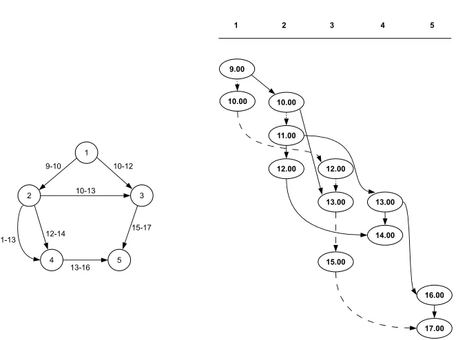
The time-expanded model is based on the following transformation. Each ele-mentary connection𝑒= (𝑠, 𝑡, 𝑑, 𝑎) induces a copy of the source node 𝑠 tagged with the departure time stamp𝑑and a copy of the target node𝑡tagged respec-tively with the arrival time stamp 𝑎. Thus, the initial connections become the connections between a pair of copies according to their time stamps.

Next, for each station𝑠of the initial network all its copies will be captured and ordered ascending their time stamps. Let𝑣1, . . . , 𝑣𝑘be the copies of𝑠in that order. Then, there is a set of stay-edges (𝑣𝑖, 𝑣𝑖+1), 𝑖= 1, . . . , 𝑘−1, connecting

the two subsequent copies within a station and representing waiting time at that station between two time events. Thus, given a graph (𝑆, 𝐸), where𝑆 is a set of stations and𝐸 is a set of edges or elementary connections, the time-expanded model will include as many as 2∣𝐸∣ − ∣𝑆∣stay-edges.

The example in Fig. 1 illustrates the transformation of an initial network to the time-expanded model. The timetable consists of five stations and seven elementary connections between these stations. The time stamps at the edges represent the departure and arrival time of the given connection.

1

2 3

4 5

10-12

10-13

15-17

13-16 11-13

12-14 9-10

9.00

10.00 10.00

11.00

12.00 12.00

13.00

15.00

13.00

16.00

17.00 14.00

1 2 3 4 5

Fig. 1.An initial network and the transformed time-expanded network

The number of nodes in the time-expanded model is equal to the double number of elementary connections of the initial graph, since each connection produces a copy of its source and its target nodes. The number of edges in the time-expanded model includes the elementary connections and the stay-edge connections (cf. Table 1).

Table 1.The size of the time-expanded graph

Initial graph (𝑆, 𝐸) Time-expanded graph

Number of nodes ∣𝑆∣ 2∣𝐸∣

Number of edges ∣𝐸∣ ≤3∣𝐸∣ − ∣𝑆∣ ≤3∣𝐸∣

3.2 EAP with the Time-Expanded Model

3.3 MNTP with the Time-Expanded Model

The Dijkstra _{algorithm can be also used for solving MNTP with the} time-expanded model. The edges between copies of different stations are assigned a weight of 1, and stay-edges are assigned a weight of 0. Starting at the first possible copy of a source station, the shortest path to a copy of a target station yields a solution of MNTP. The complexity of MNTP with the time-expanded model coincides with the complexity of EAP, since it uses the same algorithm. We remark that the above described applications of the time-expanded model refer to the earliest ideas of the time-expanded approach. Recently, many speed-up techniques for EAP and MNTP have been developed. The extensions and improvements of the time-expanded approach and shortest-path algorithms are described in [2, 5, 7, 11, 12]. In this paper our approach for solving EAP and MNTP is only compared to the original formulations of the time-expanded model and the shortest-path algorithms. The comparison to the newest im-provements of the time-expanded and time-dependent model should be made in future research.

4 Our Approach: The Edge-Converted Model

In this section we will describe a new model for timetable information. Similar to the time-expanded approach, we use a transformation of the initial network to obtain a static structure supporting well known algorithms, such asDijkstra or breadth-first search. The core idea of our approach is to convert the initial elementary connections to nodes. Therefore we call it edge-converted approach. The whole transformation routine is listed below:

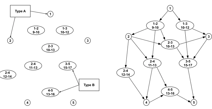
Step 1.At first we take all the stations of the initial network as new nodes. We call these nodestype A nodes.

Step 2. Then for every elementary connection 𝑒 = (𝑠, 𝑡, 𝑑, 𝑎), a new node that gets all four parameters of the edge𝑒will be created. We call these nodes

type B nodes(see Fig. 2).

Step 3. Now we connect type A nodes to type B nodes according to the next two rules.

a) There is an outgoing edge from a type A node 𝑢 to a type B node 𝑣 = (𝑠, 𝑡, 𝑎, 𝑑) if 𝑢=𝑠.

b) There is an outgoing edge from a type B node 𝑣 = (𝑠, 𝑡, 𝑎, 𝑑) to a type A node 𝑢if𝑡=𝑢 (see Fig. 2).

Step 4.Next, we add several edges connecting type B nodes with each other. There are four conditions for the existence of an edge between two type B nodes 𝑢= (𝑠𝑢, 𝑡𝑢, 𝑑𝑢, 𝑎𝑢) and 𝑣= (𝑠𝑣, 𝑡𝑣, 𝑑𝑣, 𝑎𝑣):

a) 𝑡𝑢 =𝑠𝑣 b) 𝑎𝑢≤𝑑𝑣

1 2 3 4 5 1-2 9-10 1-3 10-12 4-5 13-16 2-4 12-14 2-4 11-13 2-3 10-13 3-5 15-17 Type A Type B 1 2 3 4 5 1-2 9-10 1-3 10-12 4-5 13-16 2-4 12-14 2-4 11-13 2-3 10-13 3-5 15-17

Fig. 2. Generation of nodes in the converted model (left) and the complete edge-converted graph for the initial network from Fig. 1 (right)

d) For all type B nodes𝑤= (𝑠𝑤, 𝑡𝑤, 𝑑𝑤, 𝑎𝑤), if𝑠𝑤 =𝑠𝑣,𝑡𝑤 =𝑡𝑣, and 𝑎𝑢≤𝑑𝑤, then𝑎𝑤≥𝑎𝑢.

The complete edge-converted graph from the example in Fig. 1 is depicted in Fig. 2.

A route between two nodes (independent of their type) is defined as a usual path in the edge-converted graph. We start with some initial observations on the edge-converted graph.

Observation 2

1. The connections between two type B nodes represent a transfer possibility between two elementary connections in the initial timetable.

2. If there exists a route between two type A nodes 𝑢 and𝑣, then there exists a

route which only contains type B nodes as intermediate nodes, i.e., the only

type A nodes are the source𝑢and the target𝑣. Thus, the length of a route is

not dependent on the network size, but only on the number of the necessary transfers (compare with Observation 1).

3. The edge-converted graph has no cycles consisting only of type B nodes.

We will use these observations in the applications below where we search some path between two type A nodes only via type B nodes.

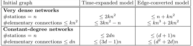
Let us calculate an estimate for this number. Given a timetable with 𝑛 stations, each station can be connected at most to𝑛−1 stations in the original network. If we assume that there are at most𝑘elementary connections between each pair of the initial stations, then, in the worst case, the edge-converted model contains𝑂(𝑘𝑛3) edges connecting type B nodes with each other.

This, however, does not happen in realistic networks. Towards a better anal-ysis, let us assume that the original network is ofconstant degree of at most𝑑, i.e., every station has at most 𝑑 ingoing and 𝑑 outgoing connections to other stations. In this case we get≤𝑑2𝑛edges for connecting type B nodes and≤2𝑑𝑛 edges for connecting type A nodes to the type B nodes. Thus, the total size of the edge-converted graph is linear in the size of the original network. This is depicted in Table 2. As the table shows, regarding realistic networks, our model contains fewer nodes, but more edges than in the time-expanded model.

Table 2.A comparison of the size of the time-expanded and edge-converted models

Initial graph Time-expanded model Edge-converted model Very dense networks

#stations =𝑛 ≤2𝑘𝑛2

≤𝑛+𝑘𝑛2 #elementary connections≤𝑘𝑛2

≤3𝑘𝑛2

−𝑛 ≤𝑘𝑛3 + 2𝑘𝑛2 Constant-degree networks

#stations =𝑛 ≤2𝑑𝑛 ≤(𝑑+ 1)𝑛

#elementary connections≤𝑑𝑛 ≤(3𝑑−1)𝑛 ≤(𝑑2 + 2𝑑)𝑛

A possible drawback of our construction is that, unlike in the time-expanded approach, we can only incorporate a fixed time horizon into the edge-converted model. Thus for practical purposes, one has to define a fixed maximal travel time and adjust the time horizon accordingly to one or several days.

5 EAP and MNTP with the Edge-Converted Model

The common approach to solve EAP or MNTP in the time-expanded approach is to use the Dijkstra _{algorithm which consumes more than linear running} time. For the edge-converted model we will describe below two algorithms for EAP and MNTP with only linear run-time. Moreover, our algorithms have the advantage of great simplicity as they implement variants of depth-first search and breadth-first search, respectively.

Our algorithms include a pre-processing step that has to be done only once. Let (𝑠, 𝑡, 𝑑) be an EAP query. We need to find a route connecting the stations 𝑠and 𝑡, starting not earlier than at the given time𝑑and providing the earliest arrival time at𝑡. The main idea of our algorithm below is to use a usual depth-first search but starting from the target node 𝑡 and moving backwards to the source𝑠. This algorithm solves the EAP if we execute the next pre-processing routine on the edge-converted model:

2. Next, given some node 𝑣 of type A or type B in an edge-converted graph, it has a set of ingoing edges{𝑒1, . . . , 𝑒𝑘}. Every edge𝑒𝑖= (𝑢𝑖, 𝑣) in this list has a start node𝑢𝑖 of type B, because there are no edges starting in type A nodes according to the previous step. We sort the set of ingoing edges for each node 𝑣 in descending order by the arrival time stamps of their start nodes𝑢𝑖.

5.1 EAP with the Edge-Converted Model

Algorithm 1 implements an inverse depth-first search on an edge-converted net-work constructed and pre-processed according to the above rules. The algorithm uses a stack 𝑆 supporting the operations push(𝑆, 𝑢) and pop(𝑆, 𝑢) which push and pop a node 𝑢 from the top of 𝑆. During the computation the algorithm maintains an array route[𝑢] which for each type B node 𝑢 points towards a subsequent connection. At the end, the fastest route from𝑠to𝑡can be read off by following the pointers in the array, starting with route[𝑠].

Algorithm 1 EAP in the edge-converted model

Require: an EAP query (𝐺, 𝑠, 𝑡, 𝑑0)

where𝐺= (𝑉, 𝐸) is an edge-converted network, 𝑠, 𝑡∈𝑉 are the start and target node, and𝑑0 is the earliest departure time

1: for all𝑣∈𝑉 do 2: route[𝑣]←nil 3: visited[𝑣]←false 4: end for

5: push(𝑆, 𝑡)

6: while𝑆 is not emptydo 7: 𝑢←pop(𝑆)

8: visited[𝑢]←true

9: if 𝑢is a type A nodethen{this only happens if𝑢=𝑡}

10: 𝑠𝑢←𝑢

11: else

12: 𝑢= (𝑠𝑢, 𝑡𝑢, 𝑑𝑢, 𝑎𝑢) is a type B node 13: end if

14: if 𝑠𝑢=𝑠then 15: route[𝑠]←𝑢

16: return route 17: end if

18: for alledges𝑒= (𝑣, 𝑢) (in descending order according to the arrival time𝑎of𝑣)do 19: 𝑣= (𝑠𝑣, 𝑡𝑣, 𝑑𝑣, 𝑎𝑣) is a type B node

20: if visited[𝑣] = false and𝑑𝑣≥𝑑0 then 21: route[𝑣]←𝑢

22: push(𝑆, 𝑣) 23: end if 24: end for 25: end while

26: return there is no connection between𝑠and𝑡starting after time𝑑0

We state the correctness of the algorithm in the following theorem.

Proof. Let𝐺be an edge-converted network and let (𝑠, 𝑡, 𝑑0) be an EAP query.

Let 𝑢1, . . . , 𝑢𝑘 be the set of predecessors of 𝑡, ordered according to the arrival time stamps of the type B nodes𝑢𝑖 (in ascending order). Each node 𝑢𝑖 is the root of a depth-first search tree𝑇𝑖 consisting of all nodes which are visited from

𝑢𝑖 in Algorithm 1. If the EAP instance (𝑠, 𝑡, 𝑑0) has a solution, then there exists

a type B node 𝑣𝑠 = (𝑠, 𝑣, 𝑑, 𝑎) such that 𝑑≥ 𝑑0 and 𝑣𝑠 is contained in one of the trees𝑇𝑖 for some 1≤𝑖≤𝑘.

We prove the correctness of Algorithm 1 by induction on the number𝑖. First note that if𝑠 is reached in line 14, then

(𝑣𝑠= route[𝑠],route[route[𝑠]], . . . , 𝑢𝑖, 𝑡)

describes the unique path from 𝑣𝑠 to 𝑡 in 𝑇𝑖. In the base case 𝑖= 1, we have

𝑣𝑠∈𝑇1. But then we have found a route from 𝑠to𝑡 which arrives at 𝑡by the

earliest possible connection in the network, and hence this route is optimal. Let now𝑣𝑠∈𝑇𝑖 with𝑖≥2. Aiming towards a contradiction, we assume that Algorithm 1 returns the route via the connections (𝑣𝑠, . . . , 𝑢𝑖), but this is not the optimal solution. This means that there exists some node𝑣′

𝑠= (𝑠, 𝑣′, 𝑑′, 𝑎′) such that 𝑑′ _{≥ 𝑑}

0 and there exists a route (𝑠, 𝑣𝑠′, . . . , 𝑢𝑗, 𝑡) which leads to an earlier arrival at𝑡. As the connections 𝑢1, . . . , 𝑢𝑘 have been ordered according to their arrival times, we have𝑗 < 𝑖. But then𝑣′

𝑠 ∈𝑇𝑗 and Algorithm 1 would have returned the route (𝑠, 𝑣′

𝑠, . . . , 𝑢𝑗, 𝑡) by the induction hypothesis.

Therefore, Algorithm 1 is correct. It runs in linear time, because every type B

node is visited at most once. ⊓⊔

In Theorem 3 the time is measured in terms of the input, i.e., in terms of the edge-converted network. As the size of the edge-converted graph is linear for constant-degree graphs (cf. Table 2), we immediately get:

Corollary 4. For constant-degree graphs, Algorithm 1 solves the EAP in linear time measured in the size of the initial network.

In comparison, usingDijkstra_{on constant-degree graphs only yields} algo-rithms with running time 𝑂(𝑛log𝑛). In real networks, each station only has a limited number of connections per time interval. Therefore, real networks will usually be close to regular graphs.

5.2 MNTP with the Edge-Converted Model

To solve MNTP with the edge-converted model we can use breadth-first search (see Algorithm 2). Starting at the source node𝑠, we find the minimum number of transfers route by reaching the target node𝑡. Instead of a stack, Algorithm 2 uses a queue 𝑄. The correctness of the algorithm can be shown by induction on the number of transfers in the optimal route from 𝑠to𝑡. Thus we get:

Theorem 5. Algorithm 2 solves the MNTP in the edge-converted model in linear time.

Again, for regular networks we obtain a linear-time bound in terms of the original network:

Algorithm 2 MNTP in the edge-converted model

Require: an MNTP query (𝐺, 𝑠, 𝑡)

where𝐺= (𝑉, 𝐸) is an edge-converted network and𝑠, 𝑡∈𝑉 are the start and target node 1: for all𝑣∈𝑉 do

2: route[𝑣]←nil 3: visited[𝑣]←false 4: end for

5: if 𝑠=𝑡then 6: return route 7: end if

8: enqueue(𝑄, 𝑠)

9: while𝑄is not emptydo 10: 𝑢←dequeue(𝑄) 11: visited[𝑢]←true

12: for alledges𝑒= (𝑢, 𝑣)do

13: if visited[𝑣] = false and𝑣= (𝑠𝑣, 𝑡𝑣, 𝑑, 𝑎) is a type B nodethen 14: route[𝑣]←𝑢

15: if 𝑡𝑣=𝑡then 16: route[𝑡]←𝑣

17: return route 18: end if

19: enqueue(𝑄, 𝑣) 20: end if

21: end for 22: end while

23: return there is no connection between𝑠and𝑡

6 Experiments

To test the performance of the algorithms for EAP and MNTP in our model we implemented the time-expanded and edge-converted model. To solve EAP and MNTP in the time-expanded model we used Dijkstra _{with a priority queue,} yielding time complexity 𝑂(𝑛log𝑛). These algorithms were tested against Al-gorithms 1 and 2 in the edge-converted model on randomly generated data.

The experiments were run on a PC with an Intel Core2Duo processor at 1.6 GHz and 2 GB RAM running Windows Vista. The algorithms were imple-mented in C++ _{compiled with a VC8 compiler on the maximum optimization} level. We used the Boost Graph Library [14] for all the graph, node, edge, and iterator classes.

6.1 Test Data Generation

We use a rectangle area to distribute a set of stations. The stations are randomly chosen in the area by assigning some 𝑥 and 𝑦 coordinates. Each station 𝑢 gets some priority𝑝(𝑢) in the interval [0,1]. The priorities are uniformly distributed among all nodes. The distance d(𝑢, 𝑣) between two stations𝑢 and 𝑣 is defined as the Euclidean distance between 𝑢 and 𝑣 in the plane.

For each pair of stations (𝑢, 𝑣) we introduce elementary connections between 𝑢and𝑣if 𝑝(d𝑢₍)_𝑢,𝑣⋅𝑝(₎𝑣) is greater than some chosen threshold. We choose the number

of these elementary connections proportional to d_(𝑢,𝑣1 ₎. The time horizon is

the travel time proportional to d(𝑢, 𝑣). The departure time at 𝑢 is uniformly distributed over the time horizon taking into account that the arrival time must also fall within the time horizon.

6.2 Performance Analysis

We ran experiments with 20, 30, 40, 50, 60, and 70 stations. As the pre-processing time increases rapidly with the number of nodes, we could not per-form experiments with many stations, for lack of hardware. For each experiment we generated the test data and counted the number of nodes and elementary connections in the initial network as well as in the time-expanded and edge-converted models. Then we solved EAP and MNTP by both approaches and measured the time. The results are shown in Table 3.

Table 3.Experimental comparison of EAP and MNTP in the time-expanded model (using

Dijkstra_{with priority queue) and in the edge-converted model (Algorithms 1 and 2)}

Initial graph Time-expanded model Edge-converted model

EAP MNTP EAP MNTP

#nodes #edges #nodes #edges

in sec. in sec. #nodes #edges in sec. in sec.

20 1048 2019 7020 11 15 1068 11434 4 34

30 2854 5336 18743 20 28 2884 52763 9 140

40 4141 7676 27016 48 64 4186 89643 15 213

50 7332 13035 46241 126 162 7382 221402 27 250

60 9140 16179 57438 143 180 9200 295835 36 321

70 10296 18108 64346 325 421 10366 351010 67 325

The results clearly show that Algorithm 1 solves EAP considerably faster than using Dijkstra _{in the time-expanded model, wheras for MNTP we} ob-tain similar running times. Comparing the size of the two models it is apparent that the edge-converted approach reduces the number of nodes by a factor of 2 whereas the number of edges drastically increases. Instead of using an ex-plicit stack, we implemented Algorithm 1 recursively which explains the better running time in comparison to Algorithm 2 which uses a queue.

7 Conclusion and Future Work

speed-up techniques are applicable in the edge-converted model. It also appears interesting to compare our model with the time-dependent approach (cf. [11] for an extensive comparison of the time-dependent and time-expanded models). Finally, in future work we would like to test the edge-converted model on larger and preferably real networks.

References

1. G. S. Brodal and R. Jacob. Time-dependent networks as models to achieve fast exact time-table queries. Electr. Notes Theor. Comput. Sci., 92:3–15, 2004.

2. D. Delling, T. Pajor, and D. Wagner. Engineering time-expanded graphs for faster timetable information. In Proc. 8th Workshop on Algorithmic Approaches for Trans-portation Modeling, Optimization, and Systems (ATMOS), 2008.

3. E. W. Dijkstra. A note on two problems in connexion with graphs. Numerische Mathe-matik, 1:269–271, 1959.

4. L. Fleischer and M. Skutella. The quickest multicommodity flow problem. In Proc. 9th International Conference on Integer Programming and Combinatorial Optimization (IPCO), pages 36–53, 2002.

5. R. Geisberger, P. Sanders, D. Schultes, and D. Delling. Contraction hierarchies: Faster and simpler hierarchical routing in road networks. InProc. 7th International Workshop on Experimental and Efficient Algorithms (WEA), pages 319–333, 2008.

6. E. K¨ohler, K. Langkau, and M. Skutella. Time-expanded graphs for flow-dependent transit times. InProc. 10th Annual European Symposium on Algorithms (ESA), pages 599–611, 2002.

7. E. K¨ohler, R. H. M¨ohring, and H. Schilling. Acceleration of shortest path and constrained shortest path computation. In Proc. 4th International Workshop on Experimental and Efficient Algorithms (WEA), pages 126–138, 2005.

8. M. M¨uller-Hannemann, F. Schulz, D. Wagner, and C. D. Zaroliagis. Timetable infor-mation: Models and algorithms. In Proc. 4th Workshop on Algorithmic Approaches for Transportation Modeling, Optimization, and Systems (ATMOS), pages 67–90, 2004. 9. A. Orda and R. Rom. Shortest-path and minimum-delay algorithms in networks with

time-dependent edge-length. Journal of the ACM, 37(3):607–625, 1990.

10. E. Pyrga, F. Schulz, D. Wagner, and C. D. Zaroliagis. Experimental comparison of shortest path approaches for timetable information. InProc. 6th Workshop on Algorithm Engi-neering and Experiments and 1st Workshop on Analytic Algorithmics and Combinatorics (ALENEX/ANALC), pages 88–99, 2004.

11. E. Pyrga, F. Schulz, D. Wagner, and C. D. Zaroliagis. Efficient models for timetable information in public transportation systems.ACM Journal of Experimental Algorithmics, 12:1–39, 2008.

12. F. Schulz, D. Wagner, and K. Weihe. Dijkstra’s algorithm on-line: An empirical case study from public railroad transport. ACM Journal of Experimental Algorithmics, 5:12, 2000.

13. F. Schulz, D. Wagner, and C. D. Zaroliagis. Using multi-level graphs for timetable infor-mation in railway systems. In4th International Workshop on Algorithm Engineering and Experiments (ALENEX), pages 43–59, 2002.

14. The Boost Graph Library. Available from http://www.boost.org.

15. D. Wagner and T. Willhalm. Speed-up techniques for shortest-path computations. In

Proc. 24th Symposium on Theoretical Aspects of Computer Science, pages 23–36, 2007. 16. D. Wagner, T. Willhalm, and C. D. Zaroliagis. Geometric containers for efficient