Identification of radius-vector functions of interface evolution for star-shaped crystal growth

This is a repository copy of

Identification of radius-vector functions of interface evolution

for star-shaped crystal growth

.

White Rose Research Online URL for this paper:

http://eprints.whiterose.ac.uk/74673/

Monograph:

Zhao, Y., Coca, D., Billings, S.A. et al. (4 more authors) (2010) Identification of

radius-vector functions of interface evolution for star-shaped crystal growth. Research

Report. ACSE Research Report no. 1022 . Automatic Control and Systems Engineering,

University of Sheffield

[email protected] https://eprints.whiterose.ac.uk/ Reuse

Unless indicated otherwise, fulltext items are protected by copyright with all rights reserved. The copyright exception in section 29 of the Copyright, Designs and Patents Act 1988 allows the making of a single copy solely for the purpose of non-commercial research or private study within the limits of fair dealing. The publisher or other rights-holder may allow further reproduction and re-use of this version - refer to the White Rose Research Online record for this item. Where records identify the publisher as the copyright holder, users can verify any specific terms of use on the publisher’s website.

Takedown

If you consider content in White Rose Research Online to be in breach of UK law, please notify us by

Identification of Radius-Vector Functions of Interface Evolution

for Star-Shaped Crystal Growth

Y. Zhao, D.Coca, S.A. Billings, Y.Guo, R.I.Ristic, L.L.De Matos,

A.Dougherty

Research Report No. 1022

Department of Automatic Control and Systems Engineering

The University of Sheffield

Mappin Street, Sheffield,

S1 3JD, UK

Identification of Radius-Vector Functions of Interface Evolution

for Star-Shaped Crystal Growth

Y.Zhao, D.Coca, S.A.Billings, Y.Guo ∗_{, R.I.Ristic, L.L.DeMatos} †_{, A.Dougherty}‡

October 26, 2010

Abstract

This paper introduces a new method based on a radius-vector function for identifying

the spatio-temporal transition rule of star-shaped crystal growth directly from experimental

crystal growth imaging data. From the morphology point of view, the growth is decomposed

as initial conditions, uniform growth and directional growth, which is represented by a static

polynomial model based on the Fourier expansion. A recursive model is also introduced

to help understand the dynamic characteristics of the observed systems. The applicability

of the proposed approach is demonstrated using data from a simulation and from a real

crystal growth experiment.

1

Introduction

Considerable theoretical and experimental effort has been expended in an attempt to develop a better understanding of growth processes that are driven by surface energy at the curved phase boundary. One of the most common examples of such a process is the growth of crystals. The crystal growth process starts at the nucleation stage, when several atoms or molecules form clusters that subsequently grow by the addition of other atoms. Patterns generated by growth processes are typically characterized in terms of characteristic length, (such as the thickness of a branch, the distance between two side-branches and the curvature of the branch tips) and crystal growth rate. The investigation of the time evolution of the characteristic lengths, using experimental, theoretical and computer simulation methods can provide valuable information on the mechanisms of crystal growth [R.Kobayashi, 1993; Dougherty and Lahir, 2005; Bisker-Leib and Doherty, 2001, 2003].

∗_{Department of Automatic Control and System Engineering, University of Sheffield, UK.}

†_{Department of Chemical and Process Engineering, University of Sheffield, UK.}

A wide range of mathematical models have already been developed to simulate the growth dynamics of crystals. The Eden model [Eden, 1956a,b], initially developed to investigate the growth of biological cell colonies, and the diffusion-limited aggregation (DLA) model [Witten and Sander, 1981], one of the most striking examples of the generation of a complex disorderly pattern by a simple model, have been widely used in biology, colloid science and materials science [T.Williams and R.Rjerknes, 1972; D.Mollison, 1972; P.Meakin, 1983; M.J.Vold, 1963]. Recently, the Phase Field Model [R.Kobayashi, 1993] has been widely used in the simulation of the growth of alloys [George and Warren, 2002; Takaki et al., 2005; Hou et al., 2005]. More-over, the Sharp Interface Model [Maalmi et al., 1995; M and M, 2007], the Boolean Model for Snowflake Growth [S.A.Wolfram, 2002] and the Cellular Automata Model [Zhao et al., 2009] have also been developed to model growth processes. A parabolic model with fourth-order cor-rection was introduced to fit to the profile of the tips of NH4Cl dendrites [Dougherty and Lahir, 2005; A and T, 2007]. However, very few authors have studied the problem of how to obtain simple empirical mathematical descriptions directly from observed experimental growth data. The identification of the models of crystal growth directly from experimental observation is a powerful tool for understanding crystal growth mechanisms and for unravelling the complex relationships between various growth patterns and the environmental variables that control this process allowing for the development of robust model-based feedback control schemes. Initially, this paper introduces a general model based on the polar coordinates which is param-eterised by the arc length of contour. Theoretically, this model can describe an arbitrary closed contour. This paper then proposes a new approach to identify a radius-vector based function, as a particular case of the general model, directly from experimental observations (imaging) for star-shaped growth, which typical arises in the early stages of crystal growth. The star-shape

is defined as: for any point in the contour p the whole line segment from the reference point

O to plies within the pattern. The reference point O is located in the interior of the contour. It is a criterion to test if a particular data set can be modelled by the proposed radius-vector based model. The distance from the pole of the polar coordinates is modelled by introducing a Fourier expansion, and the evolution characteristics are represented by a recursive model ob-tained by choosing the significant terms using the Error Reduction Ratio from the Orthogonal Least Square method [M.Korenberg and S.A.Billings, 1988].

2

Radius-Vector Function

Most currently studied methods in modelling crystal growth are based on cartesian coordinates. From the morphology point of view, this paper introduces a radius-vector based model in polar coordinates to identify the crystal growth processes in a polynomial form in terms of the characteristics of the growth speed of the interface.

In two dimensions, at a time t, the crystal is assumed to occupy an open subset Ωt ∈ R2

with contour represented by an evolving closed curve γ(t) separating its interior and exterior. Now consider the closed contour curve in polar coordinates, which can be mapped as ¯x : [0, S) ×(0, T) → R2 such that ¯x(s, t) = r(s, t), θ(s, t)

is a point on the curve γ(t) and ¯

x(0, t) = ¯x(S, t), 0≤ s≤S, where r denotes the distance to the pole, θ denotes the positive angle required to reach the point from 0◦ _{and S denotes the arc length of γ(t). The curve}

is parameterised so that the interior is on the left in the direction of increasing s (counter clockwise parameterisation). If r(s, t), θ(s, t)

are given, then evolution of the contour can be completely reconstructed.

In this paper, to simplify the problem,θ(s, t) is assumed to be independent totand is expressed as:

θ(s, t) =θ(s) = s

S ×2π (1)

As S is a constant, s is linear in θ. Therefore, r(s, t) is a function between the radius r and the vector θ which determines the spatio-temporal evolution of the interface. In other word, the map γ(t)→ r(s, t), θ(s, t)

can be simplified as the map γ(t)→r(s, t).

From the morphology point of view, this paper introduces a polynomial model expressed as

r(s, t) =v(s, t) +h(t) +c(s) (2) where c(s) denotes the initial conditions for the growth,h(t) denotes a uniform growth in all directions and v(s, t) is the growth function. Becausev(s, t) is a periodic function in θ(s) due to

v(s, t) =v(s+S, t) (3)

a Fourier expansion can be used to replace it, and Eq. (2) can then be rewritten as:

r(s, t) =P

k

gk,1(t)coskθ(s) +gk,2(t)sinkθ(s)

+h(t) +c(s) (4) where gk,1(t), gk,2(t) are the Fourier coefficients that are functions of time t, which extends

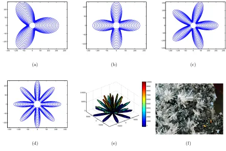
non-star-shaped patterns when θ(s) is chosen to be nonlinear in S. Moreover, this model can easily be extended to the three-dimensional case, which will be investigated in a further study. Starting from a circle, the interface displacement of four simulation examples in the two-dimensional case with different growth roles are shown in Figure 1.(a)-(d), which demonstrate that this kind of model can simulate complex crystal forms with an arbitrary number of branches. Figure 1.(e) also shows an example in three-dimensions where the form and dis-tribution of the branches are very similar to the real crystal cluster, shown in Figure 1.(f).

−150 −100 −50 0 50 100 150 200 −100 −50 0 50 100 (a)

−150 −100 −50 0 50 100 150 −100 −50 0 50 100 (b)

−150 −100 −50 0 50 100 150 200 −150 −100 −50 0 50 100 150 (c)

−150 −100 −50 0 50 100 150 −100 −50 0 50 100 (d) −5000 0 5000 −5000 0 5000 0 5000 10000 0 1000 2000 3000 4000 5000 6000 7000 8000 9000 10000 (e) (f)

Figure 1: (a)-(d) Interface displacements of simulation examples by Eq. (4) in two-dimensions; (e) Snapshot of

simulation example in three-dimensions; (f) Snapshot of a real crystal cluster.

3

Identification of the Radius-vector Function

The derivative from Eq. (4) is given by: ˙

r(s, t) =P

k

˙

gk,1(t)coskθ(s) + ˙gk,2(t)sinkθ(s)

+ ˙h(t) (5) A discrete recursive model therefore can be expressed as

r(s, t) =P

i,kai,kr(s, t−i)coskθ(s) +Pi,kbi,kr(s, t−i)sinkθ(s) +h(t) +d(s) (6)

where ai,k, bi,k are the unknown Fourier coefficients. Eq. (6) can be identified directly from

observed data using term selection and parameters estimation methods, and the many analytic methods which have been developed for dynamic models can then be applied to analyse and to help understand the observed system.

Given a group of observed data (rj, θj, tj), where j denotes the time index, the actual terms

of Eq.(6) can be selected using the Orthogonal Least Squares routine (OLS) by ranking the candidate terms based on the Error Reduction Ratio (ERR), and then estimating the unknown parameters.

The selection of candidate terms is always very important in identification of a spatio-temporal system [Zhao and Billings, 2006]. There are two parameters which determine the candidate terms: D, the maximal time lag and K, the maximal value of k. The selection of K can be determined by the number of the branches andDis always chosen 1 in this paper. An example of the identification approach using simulation data will be employed to illustrate the approach. Starting from a circle, sixteen frames were generated using the rule

r(s, t) = 8tcos2_{2θ(s) + 24tsin}2_{3θ(s) +t+ 20}

The generated patterns were sampled at θby interval of 0.1 (S = 20π), and the displacement of the sampled interface is shown in Figure 2.(a).

Because there are six branches in the pattern, the initial candidate term set was therefore chosen as

{1,

cosθ(s), cos2θ(s), ..., cos6θ(s), sinθ(s), sin2θ(s), ..., sin6θ(s), r(s, t−1),

r(s, t−1)cosθ(s), r(s, t−1)cos2θ(s), ..., r(s, t−1)cos6θ(s), r(s, t−1)sinθ(s), r(s, t−1)sin2θ(s), ..., r(s, t−1)sin6θ(s)}

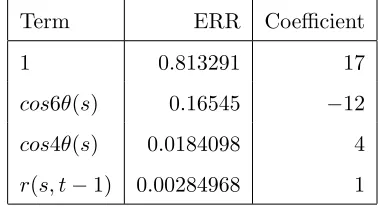
The selected terms and corresponding coefficients produced by OLS are shown in Table 1. The dynamic model can then be expressed using Eq.(7) as

−600 −400 −200 0 200 400 600 −500

−400 −300 −200 −100 0 100 200 300 400 500

(a)

−600 −400 −200 0 200 400 600 −500

−400 −300 −200 −100 0 100 200 300 400 500

(b)

Figure 2: (a)Observed data from a simulation example ; (b)Displacement of multi-step ahead prediction using

the identified model (Eq.(7)).

Table 1: Results for the identification of simulation data using OLS

Term ERR Coefficient

1 0.813291 17

cos6θ(s) 0.16545 −12

cos4θ(s) 0.0184098 4

r(s, t−1) 0.00284968 1

To evaluate the identified model, starting from the same initial conditions as the simulation, for a group of patterns the multi-step ahead predictions using Eq.(7) and the displacement of the predicted interface were computed and are shown in Figure 2.(b). Inspection of the initial data and the multi-step ahead predictions shows that the identified model can fully describe the observed system. This is also reflected by the fact that the sum of the ERR values of the selected terms is 1, as shown in Table 1.

(a) (b)

Figure 3: (a) Displacement of the crystal interfaces for 16 time steps; (b) A snapshot of the crystal at time step

16.

(a)

−150 −100 −50 0 50 100 150 200 −150

−100 −50 0 50 100

(b)

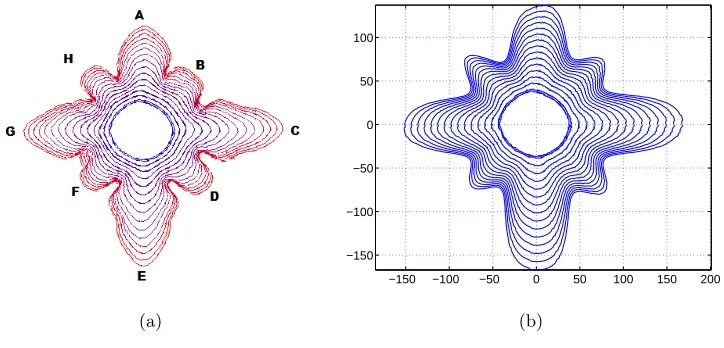
Figure 4: (a) The displacement pattern for the real example after rotating;(b) The displacement pattern

gener-ated by the identified model.

the small bumps nearby tips, the initial candidate term set was therefore chosen as

{1,

cosθ(s), cos2θ(s), ..., cos18θ(s), sinθ(s), sin2θ(s), ..., sin18θ(s), r(s, t−1),

r(s, t−1)cosθ(s), r(s, t−1)cos2θ(s), ..., r(s, t−1)cos18θ(s), r(s, t−1)sinθ(s), r(s, t−1)sin2θ(s), ..., r(s, t−1)sin18θ(s)}

using the Mean Square Error(MSE),

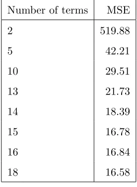
M SE(ˆr) =E(ˆr−r)2

where ˆr is the estimated value and r is the real value. Table 2 shows the MSE values of tip positions of eight branches in multi-step ahead predictions generated by models with a different number of terms. As expected, the MSE value decreases following the increment of the number

Table 2: Comparison of MSE values of multi-step ahead prediction generated by models with different numbers

of terms

Number of terms MSE

2 519.88

5 42.21

10 29.51

13 21.73

14 18.39

15 16.78

16 16.84

18 16.58

of terms. Notice that the model predictions show no significant improvement if the number of terms is larger than 15. For this example, the algorithm has therefore selected the most significant 15 terms from a total set of 56 possible model terms.

The final description of the identified model, the parameters of which were estimated using OLS after term selection, is presented in Table 3. To evaluate the identified model, starting from the same first and second frames as the observed data, fourteen multi-step ahead predictions were generated, and the displacement of the interfaces is shown in Figure 4.(b). A compari-son between Figure 4.(a) and (b) shows that the identified model captures the main growth characteristics, such as the number of branches, asymmetrical growth speed among branches etc.. Moreover, the interface of the 14th_{predicted frame is very close to the real data, which is}

always very difficult to achieve for multi-step ahead predictions. Figure 5 shows a comparisons of the radius-vector function between the reconstructed data and the real data at different times, where the dot curves indicate the contours from reconstructed data and the solid curves indicate the contours from real data. This also clearly indicates that the reconstructed contours are geometrically close to the contours of the real data.

Table 3: Results for the identification of the real data using OLS

Term ERR Coefficient

r(s, t−1) 0.9983 0.965883 1 0.000277527 7.55169

r(s, t−1)cos4θ(s) 0.000289163 0.0283955

cos8θ(s) 0.000126877 0.0834899

r(s, t−1)sinθ(s) 2.04141e−005 −0.00607122

cosθ(s) 1.16115e−005 0.395276

r(s, t−1)cos12θ(s) 1.03818e−005 −0.0168275

r(s, t−1)cos8θ(s) 9.21077e−006 0.019635

r(s, t−1)sin3θ(s) 8.7034e−006 0.0044834

r(s, t−1)cos5θ(s) 4.20299e−006 0.00309449

r(s, t−1)sin6θ(s) 4.13019e−006 0.00299367

cos12θ(s) 3.55307e−006 0.806516

sin5θ(s) 3.50071e−006 −0.227734

r(s, t−1)cos10θ(s) 2.59922e−006 0.00241942

cos3θ(s) 1.00339e−006 0.120467

0 1 2 3 4 5 6 7

40 60 80 100 120 140 160 180

r

t=3 t=10 t=16

Figure 5: Radius vs vector of real data and reconstructed data at different times

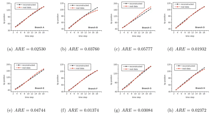
2 4 6 810 12 14 16 18 30 60 90 120 150 Branch A reconstructed real data tip position time step

(a)ARE_{= 0}.₀₂₅₃₀

2 4 6 8 10 12 14 16 18 40 60 80 100 120 reconstructed real data Branch B tip position time step

(b)ARE_{= 0}.₀₃₇₆₀

2 4 6 8 10 12 14 16 18 40 80 120 160 200 Branch C tip position time step reconstructed real data

(c)ARE_{= 0}.₀₅₇₇₇

2 4 6 810 12 14 16 18 40

60 80 100

120 reconstructed

real data

Branch D

tip position

time step

(d) ARE_{= 0}.₀₁₉₃₂

2 4 6 8 10 12 14 16 18 40

80 120 160

200 reconstructed real data

Branch E

tip position

time step

(e)ARE= 0.04744

2 4 6 8 10 12 14 16 18 40 60 80 100 120 Branch F reconstructed real data tip position time step

(f) ARE= 0.01374

2 4 6 8 10 12 14 16 18 40 80 120 160 Branch G reconstructed real data tip position time step

(g)ARE= 0.03084

2 4 6 8 10 12 14 16 18 40 60 80 100 120 Branch H reconstructed real data tip position time step

(h) ARE= 0.02372

Figure 6: Comparison of real position and predicted position of each tip over time

Figure 6 along with the corresponding averaged relative error(ARE). ARE can be expressed as

ARE(ˆr) =E(|rˆ−r|

r )

All values of ARE for the eight branch tips are below 0.06, which indicates that the model describes the tip growth well.

4

Conclusions

a real crystal experiment shows the accuracy of the identified model depends on the complexity of the model. To achieve an effective model with the least number of terms, the MSE was em-ployed to evaluate the performance of the models. Results of the multi-step ahead prediction clearly show the identified model can capture most growth characteristics in both spatio and temporal planes.

Both studied examples in this paper are based on star-shaped patterns, which is normal in the early stages of crystal growth. In this case,θ(s) is linear insand independent of time t. This model can also describe non-star-shaped patterns when θ(s) is nonlinear insor dependent on

t. In this case, the identification includes not only the determination of r(s, t), but also the determination of θ(s, t). This will be studied in future to consider more characteristics to de-scribe the later stage - dendritic formation. Identification of real systems is often very difficult because of the many factors involved, such as rotation of the crystal, aberrations in the lens or other equipment factors. Predicting anything many steps ahead is always going to show up increasing errors as the prediction horizon increases. This is an inevitable consequence of slight model errors, noise effects etc. Many more experiments need to be conducted and the link between the identified model and the environmental and control parameters needs to be investigated in further studies.

Acknowledgment

The authors gratefully acknowledge that part of this work was financed by Engineering and Physical Sciences Research Council(EPSRC), UK, and by the European Research Council(ERC).

References

Dougherty A and Nunnally T. The transient growth of ammonium chloride dendrites. Journal of Crystal Growth, 300(2):467–472, 2007.

V Bisker-Leib and M. F. Doherty. Modeling the crystal shape of polar organic materi-als:prediction of urea crystals grown from polar and nonpolar solvents. Crystal Growth & Design, 1(6):455–461, 2001.

V Bisker-Leib and M. F. Doherty. Modeling crystal shape of polar organic materials: Applica-tions to amino acids. Crystal Growth & Design, 3(2):222–237, 2003.

Andrew Dougherty and Mayank Lahir. Shape of ammonium chloride dendrite tips at small supersaturation. Journal of Crystal Growth, 274(1-2):233–240, 2005.

Murray Eden. A two-dimensional growth process. 4th. Berkeley symposium on mathematics statistics and probability, 4:223–239, 1956a.

Murray Eden. A probabilistics model for morphogenisis. Symposium on imformation theory in bilogy, 29-31:359–370, 1956b.

WL George and JA Warren. A parallel 3d dendritic growth simulator using the phase-field method. Journal Of Computational Physics, 177(2):264–283, 2002.

H Hou, DY Ju, and YH Zhao. Numerical simulation for dendrite growth of binary alloy with phase-field method. Journal Of Materials Science & Technology, 20(1):45–48, 2005.

Buchmann M and Rettenmayr M. Rapid solidification theory revisited - a consistent model based on a sharp interface. Scripta Materialia, 57(2):169–172, 2007.

M Maalmi, A Varma, and WC Strieder. The sharp interface model - zero-order reaction with volume change. Industrial & Engineering Chemistry Research, 34(4):1114–1125, 1995. M.J.Vold. Computer simulation of floc formation in a colloidal suspension. Journal of colloid

science, 18:684–695, 1963.

M.Korenberg and S.A.Billings. Orthogonal parameter estimation algorithm for nonlinear stochastic systems. International journal of control, 48(1):193–210, 1988.

P.Meakin. Cluster-growth processes on a two-diemensional lattice. Physical Review, B28: 6718–6732, 1983.

R.Kobayashi. Modelling and numerical simualtions of dendritic crystal growth. Phsical D, 63: 410–423, 1993.

S.A.Wolfram. A new kind of science. Champaign: Wolfram Media, 2002.

T Takaki, T Fukuoka, and Y Tomita. Phase-field simulation during directional solidification of a binary alloy using adaptive finite element method. Journal Of Crystal Growth, 283(1-2): 263–278, 2005.

T.A. Witten and L.M. Sander. Diffusion-limited aggregation, a kinetic critical phenomenon.

Physical Review Letters, 47:1400–1403, 1981.

Y. Zhao and S.A. Billings. Neighborhood detection using mutual information for the identifi-cation of cellular automata. IEEE Transactions on Systems, MAN, and CyberneticsPart B, 36(2):473–479, 2006.

Y. Zhao, S.A. Billings, D. Coca, R.I.Ristic, and L.DeMatos. Identification of the transition rule in a modified cellular automata model: The case of dendritic nh4br crystal growth.