LTH1043
Gradient flows in three dimensions
I. Jack1, D.R.T. Jones2 and C. Poole3
Dept. of Mathematical Sciences, University of Liverpool, Liverpool L69 3BX, UK
Abstract
The a-function is a proposed quantity defined for quantum field theories which has a monotonic behaviour along renormalisation group flows, being related to theβ -functions via a gradient flow equation involving a positive definite metric. We demon-strate the existence of a candidatea-function for renormalisable Chern-Simons theo-ries in three dimensions, involving scalar and fermion fields, in both non-supersymmetric and supersymmetric cases.
1
Introduction
It is natural to regard quantum field theories as points on a manifold with the couplings
{gI} as co-ordinates, and with a natural flow determined by the β-functions βI(g). At fixed points the quantum field theory is scale-invariant and is expected to become a con-formal field theory. It was suggested by Cardy [1] that there might be a four-dimensional generalisation of Zamolodchikov’s c-theorem [2] in two dimensions, such that there is a functiona(g) which has monotonic behaviour under renormalisation-group (RG) flow (the strong a-theorem) or which is defined at fixed points such that aUV−aIR >0 (the weak
a-theorem). It soon became clear that the coefficient of the Gauss-Bonnet term in the trace of the energy-momentum tensor is the only natural candidate for the a-function in four dimensions. A proof of the weak a-theorem has been presented by Komargodski and Schwimmer [3] and further analysed and extended in Refs. [4, 5].
In other work, a perturbative version of the strong a-theorem has been derived [6, 7] from Wess-Zumino consistency conditions for the response of the theory defined on curved spacetime, and withx-dependent couplingsgI(x), to a Weyl rescaling of the metric [8] (see Ref. [7] for a comprehensive set of references). 4 The essential result is that we can define
a functionA which satisfies the crucial equation
∂IA=TIJβJ, (1.1)
for a function TIJ which may in principle be computed perturbatively within the theory extended to curved spacetime and x-dependent gI. Eq. (1.1) implies
µ d
dµA=β I ∂
∂gIA=GIJβ
IβJ (1.2)
where GIJ =T(IJ); thus verifying the strong a-theorem so long asGIJ is positive-definite. (We shall use the notation A rather thana in anticipation of generalising this equation to three dimensions.)
In odd dimensions there is no Weyl anomaly involving curvature invariants in the usual fashion; though it does appear in the case of a CP-violating theory with x-dependent couplings [11]. Therefore it is not obvious that this approach to the a-function is viable (recall that ind= 2 andd= 4 the natural candidates for thea-function are associated with Weyl anomaly terms of the generic formR and R2 (the Gauss-Bonnet term) respectively).
However, the general local RG approach has been used in three dimensions in Ref. [11] to obtain other consistency conditions amongst RG quantities. Moreover, it has been proposed that the free energy in three dimensions may have similar properties to the four-dimensional a-function, leading to a conjectured “F-theorem” [12–14]. It has been shown that for certain theories in three dimensions, the free energy does indeed decrease monotonically along RG trajectories. It has also been argued on general grounds that the
4This approach has been extended to six dimensions in Refs. [9], and other relevant work on six
β-functions should obey a gradient flow equation in the neighbourhood of conformal fixed points, with a metric in Eq. (1.1) equal to the unit matrix to lowest order.
In this paper we take a different approach by explicitly constructing a three-dimensional “A-function”. We consider a range of renormalisable theories in three dimensions for which theβ-functions have been computed at lowest (two-loop) order. This includes general non-supersymmetric abelian and SU(n) Chern-Simons theories, together with the supersym-metric SO(n) Chern-Simons theory (the examples of supersymmetric SU(n) and Sp(n) being somewhat trivial). Using the β-functions, we show by explicit construction the exis-tence of a function A satisfying Eq. (1.1) for a metric which is at lowest order (and hence perturbatively) positive definite. This is of course the method employed in the classic work of Ref. [15]. The exact relationship of our A-function with the F-function of Ref. [12–14] is unclear. Certainly an important new feature of our results is that they appear to pass some important higher-order (four-loop) checks. In order to elucidate this further we con-sider a more general (but ungauged) theory where the relation of theA-function with the β-functions is more transparent.
2
Two-loop results
We start with the abelian Chern-Simons theory with Lagrangian [16] L= 12µνρAµ∂νAρ+|Dµφj|2+iψjDψˆ j
+αψjψjφ∗kφk+βψjψkφ∗kφj +14γ(ψjψ ∗
kφjφk+ψ ∗ jψkφ∗jφ
∗
k)−h(φ ∗
The two-loop β-functions were computed in Ref. [16] and were given as βα(2) = 83n+ 2α3+163 α2β+ 83n+ 3αβ2+ (n+ 2)β3+ 41 83n+ 173αγ2
+34(n+ 2)βγ2+ 3β2g2+14γ2g2−2
3(20n+ 31)αg
4−8βg4−8(n+ 2)g6,
ββ(2) = 83n+ 6α2β+ 3n+163 αβ2+ 23n+ 1β3+34(n+ 2)αγ2 +14 83n+ 173
βγ2−3nβ2g2+14(n+ 2)γ2g2− 2
3(8n+ 31)βg 4,
βγ(2) = 83n+ 6α2γ+ 6n+343 αβγ+ 83n+ 6β2γ+ 16(n+ 1)γ3 + 4αγg2+ 2(n+ 1)βγg2− 2
3(2n−5)γg 4,
βh(2) = 12(3n+ 11)h2+ 4h[4nα2+ 8αβ + (n+ 3)β2] + (n+ 4)hγ2 −4(5n+ 16)hg4
−[4nα4+ 16α3β+ 4(n+ 5)α2β2+ 4(n+ 3)αβ3 + (n+ 3)β4]
−[(n+ 6)α2+ (3n+ 11)(αβ +12β2)]γ2− 1
16(n+ 3)γ 4−
2(α+β)γ2g2
+ 4(nα2+ 2αβ+β2)g4−γ2g4+ 8(nα+β)g6+ 4(2n+ 7)g8. (2.2) Here and elsewhere, we suppress a factor of (8π)−4 for each loop order. These two-loop
β-functions are straightforward to calculate using dimensional regularisation (DREG) with minimal subtraction; the relevant Feynman graphs have only simple poles in = 3−d, associated of course with the absence of one-loop divergences.
It is straightforward to show that the Yukawa β-functions satisfy a relation of the form Eq. (1.1) :
∂αA ∂βA ∂γA
=
n 1 0
1 n 0
0 0 14(n+ 1)
βα(2) ββ(2) βγ(2)
, (2.3)
where
A= n4 83n+ 2
α4+16 n2+ 3n+ 3
β4 +961(n+ 1)2γ4+ 83n+ 2
α3β
+13(3n2 + 8n+ 3)β3α+13(4n2+ 9n+ 8)α2β2
+121 (4n+ 9)(n+ 1)(α2+β2)γ2+ 121(9n+ 17)(n+ 1)αβγ2 + (1−n2)β3g2+ 12(n+ 1)αγ2g2+ 14(n+ 1)2βγ2g2
− n
3(20n+ 31)α
2g4− 1 3(8n
2+ 31n+ 12)β2g4
− n
3(2n−5)γ 2
g4− 2
3(20n+ 31)αβg 4−
8n(n+ 2)αg6. (2.4)
The “metric” here is clearly positive-definite (except for the special casen= 1 where there is a zero eigenvalue reflecting the equivalence of the α,β couplings in this case). Of course the metric andA-function defined by Eq. (1.1) are only defined up to an overall scale, in the absence of any known relation to other RG quantities such as Weyl anomaly coefficients.
the non-abelian SU(n) Chern-Simons theory with Lagrangian L= 12µνρAAµ∂νAAρ +
1 6gf
ABCµνρAA µA
B νA
C
ρ +|Dµφj|2+iψjDˆψj +αψjψjφ∗kφk+βψjψkφ∗kφj +14γ(ψjψ
∗
kφjφk+ψ ∗ jψkφ∗jφ
∗
k)−h(φ ∗
jφj)3, (2.5) where
Dµφj =∂µφj−igTjkAA A
µφk, (2.6)
(similarly for Dµψ) with TjkA the generators for the fundamental representation of SU(n), satisfying [TA, TB] =ifABCTC. The non-gauge interaction terms for this theory are iden-tical with those in the abelian theory of Eq. (2.1). The two-loopβ-functions for this theory were computed in Ref. [17]; we quote here the Yukawa β-functions which are given by
βα(2) = 8 3n+ 2
α3+ 16 3α
2β+ 8 3n+ 3
αβ2 + (n+ 2)β3+1 4
8 3n+
17 3
αγ2
+34(n+ 2)βγ2−αβg2+n
2−3
2n β
2g2+n2−1
8n γ
2g2
−40n
3−17n2−40n+ 62
12n2 αg
4− 5n
3+ 6n2−18n+ 8
4n2 βg
4
+3n
4−4n3 + 5n2 −8n+ 16
8n3 g
6,
ββ(2) = 83n+ 6α2β+ 3n+ 163αβ2 + 23n+ 1β3+ 34(n+ 2)αγ2 +14 83n+173 βγ2+nαβg2+β2g2+ n
2−1
4n γ
2
g2− 5(n
2−4)
4n αg
4
−22n
3−23n2−64n+ 62
12n2 βg
4− (n2 −4)(n−2)
2n2 g
6,
βγ(2) = 83n+ 6α2γ+ 6n+ 343αβγ + 83n+ 6β2γ+16(n+ 1)γ3 +(n−1)(n+ 2)
n αγg
2+(n−1)(2n+ 1)
n βγg
2
−(n−1)(2n
2−2n+ 5)
6n2 γg
4. (2.7)
The non-gauge terms in Eq. (2.7) are of course identical with those in Eq. (2.2).
The corresponding A-function (with a metric identical to that appearing in the abelian case, Eq. (2.3)), is given by
A= n4 83n+ 2α4+16 n2+ 3n+ 3β4+961 (n+ 1)2γ4 + 83n+ 2α3β +13(3n2+ 8n+ 3)β3α+ 13(4n2+ 9n+ 8)α2β2
+121(4n+ 9)(n+ 1)(α2+β2)γ2+121 (9n+ 17)(n+ 1)αβγ2 + (n2−1)hn+ 2
8n αγ
2g2+ 2n+ 1
8n βγ
2g2+ 1 2αβ
2g2+ 1
2nβ
3g2
− 20n−1
12n α
2g4−11n
2−4n−12
12n2 β
2g4− 2n
2−2n+ 5
48n2 γ 2g4
− 15n
2+ 40n−62
12n2 αβg
4
+ 3n
2−8n+ 16
8n2 αg
6− 4n3 −11n2−8n+ 16
8n3 βg
6i
Once again, the non-gauge terms are identical to those in Eq. (2.4).
We have so far not discussed the scalar β-function βh. For this we shall return to the abelian case of Eq. (2.1). We expect a relation of the form
∂hA =Xβ
(2)
h +. . . (2.9)
where in principle the right-hand side could involve the Yukawa β-functions as well. How-ever, it turns out that no such additional terms are required at this order. If we retain onlyβh in Eq. 2.9 and integrate using Eq. (2.2) (assumingX is independent ofh), we find that we need to modify A in Eq. (2.4) according to A→A+Ah where
Ah =X
h
4(3n+ 11)h3+ 2h2[4nα2+ 8αβ + (n+ 3)β2] + 1
2(n+ 4)h
2γ2−2(5n+ 16)h2g4
−h[4nα4+ 16α3β+ 4(n+ 5)α2β2+ 4(n+ 3)αβ3+ (n+ 3)β4]
−h[(n+ 6)α2+ (3n+ 11)(αβ+12β2)]γ2− 1
16(n+ 3)hγ 4−
2h(α+β)γ2g2 + 4h(nα2 + 2αβ+β2)g4−hγ2g4+ 8h(nα+β)g6+ 4h(2n+ 7)g8. (2.10) It is then clear that we need to consider higher-order contributions to Eq. (2.3), since Eq. (2.10) will yield contributions to ∂αA of the form αh2 and α3h which are produced by four-loop diagrams5. At the very least we should include four-loop contributions to βα, etc on the right-hand side of Eq. (2.3). We have accordingly computed the four-loop contributions toβ-functions forα,β,γ with one Yukawa coupling and two scalar couplings; and with three Yukawa couplings and one scalar coupling. The results are
βα(4) =h2[83(n+ 1)(n+ 2)α+ 2(n+ 2)β]
− 2
3(n+ 2)h
n
4(n+ 1)α3+ 10(n+ 2)α2β+ (2n+ 9)αβ2+ (n+ 3)β3 +14[(2n+ 11)α+ (3n+ 11)β]γ2o+. . . ,
ββ(4) = 23(n+ 2)(n+ 4)h2β
− 2
3(n+ 2)h
n
2(n+ 6)α2β+ (3n+ 10)αβ2+ (n+ 3)β3 +14[3(n+ 4)α+ (3n+ 11)β]γ2o+. . . ,
βγ(4) = 23(n+ 2)(n+ 4)h2γ− 4
3(n+ 2)hγ
(n+ 6)α2+ (3n+ 11)(αβ+ 12β2)+. . . , (2.11) where the ellipses indicate pure Yukawa contributions which we have not calculated. In general, the metric which we have given to leading order in Eq. (2.3) might be expected to have additional higher-order corrections. However, it turns out that as far as the terms inA in Eq. (2.10) are concerned, no corrections are required and provided we take
X = 16(n+ 1)(n+ 2) (2.12)
we have
∂αAh =nβα(4)+ββ(4), ∂βAh =βα(4)+nβ
(4)
β ,
∂γAh = 14(n+ 1)βγ(4). (2.13) We shall see later that we can shed more light on the situation by turning to the general (but non-gauged) case; but for the present we continue in the next section by considering the supersymmetric gauge theory.
3
The supersymmetric case
We turn to the non-abelian N = 1 supersymmetric case. Here we consider an action S =
Z
d3xd2θh−1 4(D
αΓAβ)(D
βΓAα)−
1 6gf
ABC(DαΓAβ)ΓB αΓ
C β −
1 24g
2fABCfADEΓBαΓCβΓD αΓ
E β
− 1 2(D
α
Φj+igΦkTkjAΓαA)(DαΦj −igΓBαTjlBΦl) + 14η0(ΦjΦj)2+14η1(ΦjTjkAΦk)2
i
, (3.1)
where ΓAα is a real gauge superfield and Φ a complex matter supermultiplet (once again in the fundamental representation). Note that here α and β are three-dimensional spinor indices. We have a gauge coupling g and matter couplings η0, η1. We refer the reader to
The β-functions are given by 6
βη(2)1 =(R31+12Rt1+TRCR+ 2CR2)η1+ 14TRCAg2−21Rf1(η1+g2)
− 1
4CRCA(5η1−3g 2
) + 18CA2(η1−3g2)
(η21−g4) + [TR(η12+η1g2+g4) +CR(3η12+ 4η1g2+ 3g4)
− 1 4CA(5η
2
1 + 8η1g2+ 7g4)]R21(η1−g2)
+(6R21+ 10CR+ 3TR− 23CA)η12+ (2n+ 11)η1η0
+ 2CRη1g2−(2R21+12CA)g4
η0,
βη(2)
0 =
(R30+12Rt0)η1−12Rf0(η1+g2)
(η21−g4) + [TR(η12+η1g2+g4) +CR(3η12+ 4η1g2+ 3g4)
− 1 4CA(5η
2
1 + 8η1g2+ 7g4)]R20(η1−g2)
+ [7CRη1η0+ 3(n+ 2)η20 +CRη0g2
+ 2R20(3η12−g
4) + (2C
R+ 2TR−CA)CR(η12−g 4)]η
0. (3.2)
Here the “reduction” coefficients RXi (where X takes the values 2,3, t, f and i= 0,1) are defined by
TX =RX0T0+RX1T1, (3.3)
where
T0 = (ΦΦ)2, T1 = (ΦTAΦ)2,
T2 = (ΦTATBΦ)2, T3 = (ΦTATBTCΦ)2,
Tt= (ΦTAΦ)(ΦTBTCΦ)tr(TA{TB, TC}), Tf =fEACfEDB(ΦTATBΦ)(ΦTCTDΦ). (3.4) The group invariants are defined as usual by
CR1 =TATA, TRδAB = tr(TATB), CAδAB =fACDfBCD. (3.5) As shown in Ref. [17], the reduction coefficients may be computed for the classical groups SU(n), SO(n) andSp(n); however for SU(n) the identity
TijATklA =TR(δilδkj −n1δijδkl) (3.6) yields a simple relation betweenT0 and T1, and a similar argument (with a different
iden-tity) holds for Sp(n); so that effectively η0,1 may be replaced by a single coupling. This
is not the case for SO(n), where the analogous identity to Eq. (3.6) does not reduce the number of quartic scalar invariants. In this case there is therefore potentially a non-trivial
6Since we now deal with supersymmetry, the issue of use of regularisation by dimensional reduction
result for theA-function, so we confine our attention to this gauge group for the remainder of this section. We have for SO(n) [17]
CR= 12(n−1)TR, CA= (n−2)TR
R20 = 14(n−1)TR2, R30 =Rf0 = − 18TR3(n−1)(n−2), Rt0 =Rt1 = 0,
R21=−12TR(n−2), R31= 14TR2(n
2−
3n+ 3), Rf1 = 14TR2(n−2)(n−3), (3.7) so that the β-functions of Eq. (3.2) take the form
βη(2)0 = (n−1)18TR3(5η12+ 6η1g2+ 5g4)(η1−g2) +TR2(3η
2 1 −2g
4)η 0
+12TR(7η1+g2)η20
+ 3(n+ 2)η03,
βη(2)1 =TR245η13+ 12(n−2)η12g2+ 14(3−4n)η1g4+ 12(n−2)g6
+12(n+ 14)η21 + (n−1)η1g2+12(n−2)g4
TRη0+ (2n+ 11)η1η20. (3.8)
The value ofTRdepends on the choice of scale for the representation matrices and structure constants.There are several possible convenient choices in theSO(n) case; see Ref. [20] for a discussion. It is straightforward to show that the β-functions satisfy
∂η0A
∂η1A
=
4(n+1) (n−1) 2TR
2TR 3TR2
!
βη0
βη1
, (3.9)
where
A= 3(n+ 1)(n+ 2) n−1 η
4 0 +
2
3(n+ 1)TRg 2η3
0− 1
2(7n+ 10)T 2
Rg
4η2 0
− 3
2(n+ 3)T 3
Rg
6η
0+ 6(n+ 2)TRη30η1+ 132(n+ 2)TR2η
2 0η
2 1
+ (n−1)TR2g2η02η1−12(5n−2)TR3g
4η
0η1 +32(n−1)TR3g
2η 0η12
+ 52(n+ 2)TR3η0η31+ 165(n+ 2)T 4
Rη
4
1 +121 (7n−13)T 4
Rg
2
η31
− 1
8(13n−10)T 4
Rg
4η2 1 +
1
4(n−7)T 4
Rg
6η
1. (3.10)
We see from Eq. (3.9) that the metric is again positive definite.
In Eqs. (3.9), (3.10) we have extended the range of our results to include the N = 1 supersymmetric SO(n) theory, in addition to the general abelian and SU(n) theories considered earlier. There is little to be gained from detailed consideration of the Sp(n) supersymmetric theory; since there is in this case effectively only a single coupling, the existence of an A-function satisfying Eq. (1.1) is trivially guaranteed.
Finally a word is in order concerning the relation between the generalSU(n) theory of Section 2 and the supersymmetric SU(n) theory defined in this section. One may obtain the supersymmetric SU(n) theory of Eq. (3.1) from the general lagrangian of Eq. (2.5) by imposing [17]
g → √g
2, α → 1
4n[(n−1)η0+ng
2
], β→ 1
4n[(n−1)η0−g
2
],
γ → n−1
2n (η0−g
2
), h→ η
2
0(n−1)2
where we have set η1 = 0 since again for SU(n) there is effectively only one coupling.
It is interesting that due to the replacement h ∼ η02, Ah in Eq. (2.10) will be entirely O(η06). The terms in hwhich in the general case would have yielded the two-loopβh (upon differentiation with respect to h) will now give rise (upon differentiation with respect to η0) to higher-order contributions to the metric in Eq. (1.1) multiplying the two-loop βη0.
The connection between the four-loop and two-loop β-function coefficients is no longer apparent. A full four-loop analysis (in which it would be appropriate to use DRED rather than DREG) might reveal equivalent constraints on the β-function; or alternatively the requisite relations between β-function coefficients might be an automatic consequence of supersymmetry.
4
General theory
The above results present, at first sight, persuasive evidence for ana-theorem. It is natural to consider a generalisation to a theory with arbitrary scalar and fermion content. Thus we consider the theory
L= 12[µνρAµ∂νAρ+ (Dµφi)2 +iψaDψˆ a] +14Yabijψaψbφiφj+ 6!1hijklmnφiφjφkφlφmφn (4.1) where we employ a real basis for both scalar and fermion fields. (Recall that in d = 3, ψ =ψ∗T, and there is no obstacle to decomposing ψ into real Majorana fields.)
For the purposes of this paper we shall restrict ourselves to considering the general theory in the ungauged case. The result for the two-loop Yukawa β-function may then be written as
βabij(2) =aβabij(a) +bβabij(b) +cβabij(c) +dβabij(d) +eβabij(e) , (4.2) where βabij(a−e) correspond to the tensor structures given by
βabij(a) =YacilYcdjmYdblm+YaclmYcdjmYdbil+YacjlYcdimYdblm+YaclmYcdimYdbjl, βabij(b) =YaclmYcdijYdblm,
βabij(c) =YcdikYabklYcdlj,
βabij(d) =YacijYcdlmYdblm+YadlmYdclmYcbij,
βabij(e) =YabikYcdklYdclj +YcdilYdclkYabkj, (4.3) and where
a=b=c= 2, d=e= 23. (4.4)
the three couplings α,β and γ given for β(a) by
βα(a)= 4α3+ 6αβ2+ 2nβ3+12γ2[3α+ (3n+ 4)β]
ββ(a)= 12α2β+ 6nαβ2+ 2β3+ 12γ2[3(n+ 2)α+ (2n+ 3)β]
βγ(a)= 4γ[3α2+ 3(n+ 1)αβ+ (n+ 2)β2], (4.5) for β(b,c) by
βα(b) =βα(c)= 2nα3+ 4α2β+ 2nαβ2 + 2β3+1 2γ
2[(n+ 1)α+β],
ββ(b) =ββ(c)= 2nα2β+ 4αβ2+ 12βγ2,
βγ(b) =βγ(c)= 2γ(nα2 + 2αβ+β2), (4.6) and for the anomalous dimension contributions β(d,e) by
βα(d) =βα(e) = ˜γα, ˜
γ = 2(nα2+ 2αβ +nβ2) + 12(n+ 1)γ2, (4.7) with similar results for ββ,γ(d,e). It is easy to check that upon adding the contributions to βα,β,γ from Eqs. (4.5), (4.6), (4.7), and incorporating the factors of a-e from Eq. (4.4), we obtain the β-functions given in Eq. (2.2) (upon setting the gauge coupling g = 0) up to an overall factor of 4 which we are unable to account for. Of course such an overall factor has no effect on the existence or otherwise of the A-function.
It can readily be seen that for β-functions given by Eq. (4.3), the A-function given by A=aAa+ 14bAb+14cAc+ 12dAd+ 12eAe, (4.8) where
Aa =YabijYbcklYcdikYdajl, Ab =YabijYbcklYcdijYdakl, Ac=YabijYcdjkYabklYcdli, Ad=YacijYcbijYbdlmYdalm,
Ae =YabilYbaljYcdilYdclj. (4.9) satisfies Eq. (1.1) in the form
∂A ∂Yabij
=βabij(2) , (4.10)
where we define
∂ ∂Yabij
Ya0b0i0j0 = 1
The corresponding (lowest order) contribution to the metricGIJ is therefore effectively the unit matrix in coupling space. The different tensor structures in Eq. (4.9) are depicted in Table 1 where a vertex represents a Y and full (“fermion”) and dashed (“scalar”) lines represent contractions of a, b, . . . and i, j, . . . indices, respectively. Differentiation with respect to Y therefore corresponds to removing a vertex. and is easily seen to produce a potential β-function contribution.
Aa Ab Ac Ad Ae
Table 1: Contributions to A from Yukawa couplings
Upon specialising once again to the theory of Eq. (2.1), we obtain Aa =nα4+ 4α3β+ 6nα2β2+ 2(n2+ 1)αβ3+nβ4
+ 12(n+ 1)γ2[3α2+ 3(n+ 1)αβ+ (n+ 2)β2],
Ab,c = 12[n2α4+ 4nα3β+ 2(n2+ 2)α2β2+ 4nαβ3+β4+12(n+ 1)γ2(nα2+ 2αβ+β2)], Ad,e = 12[n2α4+ 4nα3β+ 2(n2+ 2)α2β2+ 4nαβ3+n2β4
+ 12(n+ 1)γ2(nα2+ 2αβ+nβ2)]; (4.12)
and again, it may readily be checked that upon inserting these expressions into Eq. (4.8), we obtain the A-function derived in Eq. (2.4) (with, again, g = 0). So far, there is no constraint on the two-loop coefficients a–e in Eq. (4.4). This is because the symmetries of the tensor structures appearing in Eq. (4.8) imply a one-to-one relation betweenA-function contributions and Yukawa β-function contributions. This may be seen in Table 1 where in each diagram, the removal of any vertex leads to the same β-function contribution. The A-function can thus be tailored term-by-term to match any values for theβ-function coef-ficients. This situation appears likely to be unchanged if we include gauge contributions, although we have not performed the explicit calculations.
However, a crucial difference arises in the case of the scalar coupling hijklmn. The two-loop β-function forh is given by
(βh(2))ijklmn =h1β (h1)
ijklmn+h2β (h2)
ijklmn+h3β (h3)
ijklmn+h4β (h4)
ijklmn+h5β (h5)
ijklmn, (4.13) where
β(h1)
ijklmn=
1
6!(hijkpqrhlmnpqr+ perms), β (h2)
ijklmn =
1
6!(hijklpqYabmpYabnq+ perms),
β(h3)
ijklmn=
1
6!(hijklmpYabpqYabnq+ perms), β (h4)
ijklmn =
1
6!(YabijYbcklYcdmpYdapn+ perms),
β(h5)
ijklmn =
1
where “+ perms” completes the 6! permutations of the indices {ijklmn}and
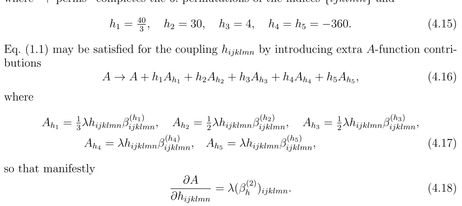
h1 = 403, h2 = 30, h3 = 4, h4 =h5 =−360. (4.15)
Eq. (1.1) may be satisfied for the couplinghijklmn by introducing extraA-function contri-butions
A→A+h1Ah1+h2Ah2 +h3Ah3 +h4Ah4 +h5Ah5, (4.16)
where
Ah1 = 1
3λhijklmnβ (h1)
ijklmn, Ah2 = 1
2λhijklmnβ (h2)
ijklmn, Ah3 = 1
2λhijklmnβ (h3)
ijklmn, Ah4 =λhijklmnβ
(h4)
ijklmn, Ah5 =λhijklmnβ (h5)
ijklmn, (4.17) so that manifestly
∂A ∂hijklmn
=λ(βh(2))ijklmn. (4.18) The different tensor structures in Eq. (4.17) are depicted in Table 2. Here differentiation with respect to h corresponds to removing a vertex with six “scalar” lines (an h-vertex) while differentiation with respect to Y corresponds as before to removing a Y vertex with two “scalar” and two “fermion” lines.
Ah
[image:13.612.68.536.119.328.2]1 Ah2 Ah3 Ah4 Ah5
Table 2: Higher order contributions to A from scalar coupling
So far there is no constraint on h1−5, just as in the case of a-e. However, when we
given by
βabij(4) =λhh2β (h2)
abij +
1 2h3β
(h3)
abij +
1 2h4β
(h4)
abij +h5β
(h5)
abij
i
+h-independent terms, β(h2)
abij =hikmnpqhjlmnpqYabkl, β(h3)
abij =hilmnpqhklmnpqYabkj +hjlmnpqhklmnpqYabik, β(h4)
abij = [(YacikYcdlmYdbnp+YacnpYcdlmYdbik)hjklmnp
+ (YackpYcdmpYdbnl+YacnlYcdmpYdbkp)hijklmn] + (i↔j), β(h5)
abij = [YacklYcdjmYdbnphiklmnp+YackpYcdlmYdbnphijklmn] + (i↔j). (4.19) Note that in the case of theh4,5diagrams in Table 2, there are two topologically inequivalent
types of Y-vertex and therefore differentiation with respect toY yields two different types of β-function contribution from each of these diagrams. Remarkably the predictions of Eq. (4.19) are verified by explicit calculations, provided λ = 901 . This agreement requires relations between two and four loop Feynman diagram pole contributions, and indeed (since as mentionedh4 andh5 each appear in two distinctβ-function contributions in Eq. (4.19))
between distinct four-loop Feynman diagrams. Yet again, these results are in agreement with the earlier explicit results, in this case those of Eqs. (2.11), (2.13). Since λ 6= 1, the overall metric in {Y, h} coupling space is not simply the unit matrix; however, this could of course be arranged by a rescaling of h.
5
Conclusions
We have demonstrated explicitly the existence of a three-dimensionalA-function satisfying Eq. (1.1) for the two-loop β-functions derived earlier in Refs. [16, 17] for a range of gauge theories coupled to scalars and fermions. Considering a more general (but ungauged) theory, we have shown that at lowest order the existence of the A-function is guaranteed irrespective of the values of the coefficients of the two-loop β-functions for the scalar and Yukawa couplings; but that this A-function also entails predictions for terms in the four-loop Yukawa β-function. We have verified that these predictions are correct. It would be interesting to investigate the relation between our results and those of Ref. [14]. These authors presented arguments based on conformal field theory for an “F-function” satisfying Eq. (1.1) at lowest order, and also found a trivial metric at this order. However, their calculations did not reveal the subtle interplay between the two and four loop β functions which is necessary for consistency in the theory with both fermions and scalars.
It is worth pointing out that these methods could also be employed in four dimensions; indeed,they already were to a considerable extent in Refs. [7, 21], though here the metric was known already at leading order from explicit computation. It would appear that in both cases the leading order metric is constant (except for a 1
It is clearly of crucial importance to carry out the full four-loop calculation (at least for the non-gauge theory) to complete the check that Eq. (1.1) is valid at this level. This computation is under way and will be reported on shortly [22]. It would also be of interest to extend our lowest order computations to a general scalar-fermion gauge theory.
Our results certainly appear to point to the all-orders validity of Eq. (1.1) in three dimensions. One way to confirm this would be to attempt to adapt the renormalisation group approach of Refs. [6]. As commented earlier, this approach is hampered by the lack of natural RG quantities to serve as the natural candidate for an A-function. One potentially significant observation is thatRφ2is dimensionless in all dimensions but there is
no clear link between the β-function for the coefficient of this quantity and the A-function as computed here.
Finally it would be interesting to test the monotonicity of our A-function beyond the weak-coupling limit, by examining its behaviour at fixed points. This could in principle be done explicitly; the fixed-point structure of the models considered in Section 2 was already mapped out in Refs. [16,17].More speculatively, one might investigate whether the values of A at fixed points in supersymmetric theories bore any relation tothe corresponding values obtained by “F-maximisation” [23].
6
Acknowledgements
We thank Hugh Osborn for a careful reading of the manuscript and several useful sugges-tions. This work was supported in part by the STFC under contract ST/G00062X/1, and CP by a STFC studentship.
References
[1] J.L. Cardy, Is there a c-theorem in four dimensions?, Phys. Lett. B215 (1988) 749. [2] A.B. Zamolodchikov, Irreversibility of the flux of the renormalization Group in a 2D
Field Theory, JETP Lett. 43 (1986) 730.
[3] Z. Komargodski and A. Schwimmer, On renormalization group flows in four dimensions, JHEP 1112 (2011) 099, arXiv:1107.3987 [hep-th] Z. Komargodski, The constraints of conformal symmetry on RG flows, JHEP 1207 (2012) 069, arXiv:1112.4538 [hep-th]. [4] M.A. Luty, J. Polchinski and R. Rattazzi, The a-theorem and the asymptotics of 4D
quantum field theory, JHEP 1301 (2013) 152, arXiv:1204.5221 [hep-th].
H. Elvang and T.M. Olson, RG flows in ddimensions, the dilaton effective action, and the a-theorem, JHEP 1303 (2013) 034, arXiv:1209.3424 [hep-th].
[6] H. Osborn, Derivation of a four-dimensional c-theorem, Phys. Lett. B222 (1989) 97; I. Jack and H. Osborn, Analogs for the c-theorem for four-dimensional renormalizable field theories, Nucl. Phys. B343 (1990) 647.
[7] I. Jack and H. Osborn, Constraints on RG flow for four-dimensional quantum field theories, Nucl. Phys. B883 (2014) 425, arXiv:1312.0428 [hep-th].
[8] H. Osborn, Weyl consistency conditions and a local renormalization group equation for general renormalizable field theories, Nucl. Phys. B363 (1991) 486.
[9] B. Grinstein, A. Stergiou and D. Stone, Consequences of Weyl consistency conditions, JHEP 1311 (2013) 195, arXiv:1308.1096 [hep-th];
B. Grinstein, A. Stergiou, D. Stone and M. Zhong, A challenge to thea-theorem in six dimensions, arXiv:1406.3626 [hep-th];
B. Grinstein, A. Stergiou, D. Stone and M. Zhong, Two-loop renormalization of multi-flavor φ3 theory in six dimensions and the trace anomaly, arXiv:1504.05959 [hep-th].
H. Osborn and A. Stergiou, Structures on the conformal manifold in six-dimensional theories, JHEP 1504 (2015) 157, arXiv:1501.01308 [hep-th].
[10] L. Fei, S. Giombi and I. R. Klebanov, “Critical O(N) models in 6− dimensions,” Phys. Rev. D 90 (2014) 2, 025018 arXiv:1404.1094 [hep-th];
L. Fei, S. Giombi, I. R. Klebanov and G. Tarnopolsky, “Three loop analysis of the criti-cal O(N) models in 6−dimensions,” Phys. Rev. D 91 (2015) 4, 045011, arXiv:1411.1099 [hep-th].
[11] Y. Nakayama, Consistency of local renormalization group in d= 3, Nucl. Phys. B879 (2014) 37, arXiv:1307.8048 [hep-th].
[12] D.L. Jafferis, The exact superconformal R-Symmetry extremizesZ, JHEP 1205 (2012) 159, arXiv:1012.3210 [hep-th].
[13] D.L. Jafferis, I.R. Klebanov, S.S. Pufu and B.R. Safdi, Towards theF-theorem: N = 2 field theories on the three-sphere, JHEP 1106 (2011) 102, arXiv:1103.1181 [hep-th]. [14] I.R. Klebanov, S.S. Pufu and B.R. Safdi, F-theorem without supersymmetry, JHEP
1110 (2011) 038, arXiv:1105.4598 [hep-th].
[15] D.J. Wallace and R.K.P. Zia, Gradient properties of the RG equations in multicom-ponent systems, Annals Phys. 92 (1975) 142.
[16] L.V. Avdeev, G.V. Grigoryev and D.I.Kazakov, Renormalizations in abelian Chern-Simons field theories with matter, Nucl. Phys. B382 (1992) 561.
[18] O. Antipin, M. Gillioz, E. Mølgaard and F. Sannino, Thea-theorem for Gauge-Yukawa theories beyond Banks-Zaks, Phys. Rev. D87 (2013) 125017, arXiv:1303.1525 [hep-th]; O. Antipin, M. Gillioz, J. Krog, E. Mølgaard and F. Sannino, Standard model vacuum stability and Weyl consistency conditions, JHEP 1308 (2013) 034, arXiv:1306.3234 [hep-ph] .
[19] W. Siegel, “Supersymmetric dimensional regularization via dimensional reduction,” Phys. Lett. B 84 (1979) 193.
D. M. Capper, D. R. T. Jones and P. van Nieuwenhuizen, “Regularization by di-mensional reduction of supersymmetric and nonsupersymmetric gauge theories,” Nucl. Phys. B 167 (1980) 479.
[20] I. Jack, D.R.T. Jones, P. Kant, L. Mihaila, The four-loop DRED gauge beta-function and fermion mass anomalous dimension for general gauge groups, JHEP 0709 (2007) 058, arXiv:0707.3055 [hep-th].
[21] I. Jack and C. Poole, The a-function for gauge theories, JHEP 1501 (2015) 138, arXiv:1411.1301 [hep-th]
[22] I. Jack, D.R.T. Jones and C. Poole, in preparation.