This is a repository copy of Emulator-based control for actuator-based hardware-in-the-loop testing.
White Rose Research Online URL for this paper: http://eprints.whiterose.ac.uk/79706/
Version: Accepted Version
Article:
Gawthrop, P.J., Virden, D.W., Neild, S.A. et al. (1 more author) (2008) Emulator-based control for actuator-based hardware-in-the-loop testing. Control Engineering Practice, 16 (8). 897 - 908. ISSN 0967-0661
https://doi.org/10.1016/j.conengprac.2007.10.009
[email protected] Reuse
Unless indicated otherwise, fulltext items are protected by copyright with all rights reserved. The copyright exception in section 29 of the Copyright, Designs and Patents Act 1988 allows the making of a single copy solely for the purpose of non-commercial research or private study within the limits of fair dealing. The publisher or other rights-holder may allow further reproduction and re-use of this version - refer to the White Rose Research Online record for this item. Where records identify the publisher as the copyright holder, users can verify any specific terms of use on the publisher’s website.
Takedown
If you consider content in White Rose Research Online to be in breach of UK law, please notify us by
Control Engineering Practice 16 (2008) 897–908
Emulator-based control for actuator-based
hardware-in-the-loop testing
P.J. Gawthrop
aD.W. Virden
bS.A. Neild
bD.J. Wagg
b,1aCentre for Systems and Control and Department of Mechanical Engineering, University
of Glasgow, GLASGOW. G12 8QQ Scotland.
bDepartment of Mechanical Engineering, Queens Building, University of Bristol, Bristol
BS8 1TR, UK.
Abstract
Hardware-in-the-loop (HWiL) is a form of component testing where hardware components
a linked with software models. In order to test mechanical components an additional
trans-fer system is required to link the software and hardware subsystems. The transtrans-fer system
typically comprises of sensors and actuators and the dynamic effects of these components
need to be eliminated to give accurate results. In this paper an emulator-based control
strat-egy is presented for actuator based HWiL. Emulator-based control can solve the twin
prob-lems of stability and fidelity caused by the unwanted transfer system (actuator) dynamics.
Significantly EBC can emulate the inverse of a transfer system which is not causally
in-vertible, allowing a wider range of more complex transfer systems to be controlled. A
robustness analysis is given and experimental results presented.
Control Engineering Practice 16 (2008) 897–908 1 Introduction
Hardware-in-the-loop (HWiL) is a form of component testing where physical
com-ponents of the system communicate with software models which simulate the
be-haviour of the rest of the system (Brendecke & Kucukay , 2002; Faithfull et al. ,
2001; Zhang & Alleyne , 2005). Typically the hardware components being tested
are control systems and the method has particular applications in the automotive
in-dustry (Hong et al., 2002; Misselhorn et al., 2006; Rulka & Pankiewicz , 2005) and
a range of other applications (de Carufel et al., 2000; Ferreira et al., 2004a,b;
Gan-guli et al., 2005; Jezernik , 2005; Lambrechts et al., 2005; Mansoor et al., 2003).
In a typical hardware-in-the-loop test, the hardware component consists of a box
of electronic components which can communicate with the software models via
electrical signals exchanged using a data acquisition and control system such as
dSpace. Extending the HWiL technique to test mechanical components has been
an area of interest for some time, for example, for use in suspension development,
see (Misselhorn et al., 2006) and references therein. The main difficulty is that
con-necting a mechanical component to a software model requires the transfer of forces
and velocities, and to achieve this an additional dynamic transfer system (Wagg &
Stoten, 2001) must be included in the loop. Typically the transfer system is a set of
actuators, which will have dynamic characteristics which need to be compensated
for if the test is to be carried out in real time.
Mitigating the effect of transfer system dynamics has been studied in detail in the
1 Corresponding author. Email: [email protected]; Tel. +44 (117) 9289736, Fax:
Control Engineering Practice 16 (2008) 897–908
context of the related testing technique of real time dynamic substructuring (RTDS)
(Blakeborough et al., 2001; Darby et al., 2002; Gawthrop et al., 2005b; Horiuchi
et al., 1999; Reinhorn et al., 2004). The topic of real-time dynamic substructuring
is the subject of a recent issue of Philosophical Transactions of the Royal Society,
within which Williams & Blakeborough (2001) give an excellent introductory
re-view. Real time dynamic substructuring is an actuator based HWiL technique
(Ab-HWiL), which so far has primarily been considered for civil engineering systems.
As a result instability is a frequent problem because the systems being modelled
usually have lightly damped resonant behaviour, and any small delays in the
trans-fer system have the effect of negative damping (Horiuchi et al., 1999; Wallace et al.,
2005a).
The effect of transfer system dynamics can be mitigated by reformulating the
prob-lem as a feedback control probprob-lem, so that the techniques of robust control design
can be applied to ensure stability (Gawthrop et al., 2006), but at the cost of reduced
accuracy. In a small number of cases, the dynamics of the transfer system can be
removed from the closed loop by using an inverted model of the transfer system
dynamics — for example, using the virtual actuator approach (Gawthrop, 2004,
2005; Gawthrop et al., 2005b) — in most cases however, the transfer system is not
(causally) invertible. One of the most commonly considered examples of a
non-invertible transfer system is that of a pure time delay. A number of approaches have
been suggested to compensate for a pure delay including polynomial extrapolation
(Darby et al., 2002; Horiuchi & Konno, 2001; Wallace et al., 2005a,b), adaptive
for-ward prediction (Darby et al., 2002; Wallace et al., 2005b,b) and Smith’s predictor
Control Engineering Practice 16 (2008) 897–908
In the automotive suspension systems studied by (Misselhorn et al., 2006) the
damping levels are significantly higher than in most RTDS tests, such that phase
margin instabilities can be avoided. In fact the approach is to use PID control, and
operate in a frequency range where actuator phase lag is seen to be acceptable.
However, for mechanical components with lower damping, we believe that the
de-lay compensation techniques developed for RTDS will be of significant benefit for
actuator based HWiL. This will also apply to applications where electro-mechanical
devices or complex circuitry are used as transfer systems, with the result that the
effect of their dynamics may be significant (Driscoll et al., 2005; Zhu et al., 2005).
It will also be useful for the development and techniques such as
model-in-the-loop (Plummer , 2006; Zhu et al., 2005) and engine-in-the-model-in-the-loop (Fathy et al., 2006)
testing which are further extensions of the HWiL technique.
In this paper, we propose the use of the emulator-based control strategy for actuator
based HWiL. Emulator-based control (EBC) gives a novel and effective solution to
the twin problems of stability and fidelity caused by the unwanted transfer system
(actuator) dynamics. In particular EBC can emulate the inverse of a transfer system
which is not causally invertible. Moreover, the approach can be used with more
complex models of transfer system dynamics than have previously been studied.
This means that more accurate coupling can be obtained, leading in turn to a higher
degree of accuracy for the complete test. This will be demonstrated using an
ex-ample of the lightly damped mass-spring-damper system previously considered in
Control Engineering Practice 16 (2008) 897–908 2 Actuator based HWiL as a feedback system
This section shows that the actuator-based HWiL (AbHWiL) approach introduced
in this paper has a feedback interpretation and that standard frequency domain
re-sults (for example as discussed in the textbook of Goodwin et al. (2001)) can be
used to analyse the resultant feedback loop.
AbHWiL involves having a model in two parts, one to be tested as a hardware
com-ponent and one to be implemented as a software model. In this paper, the analysis
is accomplished in the continuous-time domain thus regarding not only the tested
component but also the software component as a physical system. The
implementa-tion of the software component (including choice of integraimplementa-tion method and sample
time) is an important issue which is not, however, covered in this paper.
Because the complete system being modelled is a physical system, each of the
two subsystems has the special mathematical property of passivity (Willems, 1972)
which can be expressed in bond graph terms (Gawthrop et al., 2005b). The
soft-ware subsystem is connected to the hardsoft-ware subsystem via a computer digital to
analogue interface driving a physical actuator; the connection is referred to as the
transfer system.
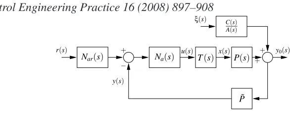
[Fig. 1 about here.]
Gawthrop et al. (2006) showed how RTDS (and hence AbHWiL) can be viewed
as a feedback system, represented in conventional block diagram form in figure
1, where P(s)is the transfer function of the hardware component, N(s)and Nr(s)
refer-Control Engineering Practice 16 (2008) 897–908
ence signal r(s)as well as the physical subsystem output y(s)) and T(s)the transfer
function of the transfer system. For the case where interface displacement is passed
from the software model to the hardware component, u(s)is the interface
displace-ment calculated by the software model, x(s) is the displacement imposed on the
hardware component, y(s)is the force required to impose the displacement x(s)on
the hardware component and r(s)is the external excitation. In the ideal situation,
T(s) =1 so that the software model output matches the hardware component
in-put exactly (and hence the AbHWiL system perfectly replicates the full physical
system). In this ideal case the closed-loop system of figure 1 has the closed-loop
transfer function yr((ss)) =Y(s)Nr(s)given by
Y(s) = N(s)P(s)
1+N(s)P(s) (1)
For the analysis in this paper the following assumptions are made:
Assumption 1 P(s)and N(s)are stable rational transfer functions.
Assumption 2 Y(s)and Nr(s)are stable.
Assumption 1 implies that
P(s) =BP(s)
AP(s)
(2)
N(s) =BN(s)
AN(s)
(3)
where the numerator and denominator of each transfer function is a polynomial in
the Laplace operator s. Assumption 2 implies that the complete physical system
being tested using the substructuring technique is stable. Define σi as the ith root
of the polynomial Aclwhere
Control Engineering Practice 16 (2008) 897–908
so that assumptions 1 and 2 implyℜσi<0∀i.
As illustrated in §4 4.2 and §5 5.3 the feedback system of figure 1 typically has
a very poor stability margin (in a sense to be defined later); thus the problem of
achieving stability and fidelity when T(s)6=1 is not trivial; this paper shows that
EBC can solve this problem in a novel way.
3 Emulator-based Control
Smith’s predictor (Marshall, 1979; Smith, 1959) is an example of a controller
us-ing a built-in mathematical model of the controlled system. Although the technique
was developed in the process industry to overcome problems in controlling
time-delay systems, it has been suggested (Agrawal & Yang, 2000; McGreevy et al.,
1998; Reinhorn et al., 2004) as method of overcoming time delay in transfer
sys-tems. Unfortunately, Smith’s predictor has serious limitations for AbHWiL/RTDS.
In particular, it has poor performance when the controlled system is lightly-damped.
Research on an alternative form of predictive control, based on stochastic time
se-ries analysis – initiated by ˚Astr¨om (1970) – lead to the development of
(discrete-time) self-tuning control ( ˚Astr¨om & Wittenmark, 1973; Clarke & Gawthrop, 1975).
Continuous-time versions of self-tuning controllers (and associated predictors) were
developed by Gawthrop (1987) and lead to the emulator-based control (EBC)
ap-proach (Gawthrop et al., 1996) which overcomes the limitations of Smith’s
predic-tor mentioned above.
Control Engineering Practice 16 (2008) 897–908
Figure 2(a) gives the basic idea of emulator based control (Gawthrop, 1987; Gawthrop
et al., 1996). The controlled system is represented by a rational transfer function
B(s)
A(s) combined with the pure time delay of τ represented by the transfer function
e−sτ; the system input (control signal) is u(s)and system output is y(s). The transfer
function CA((ss)) and the signalξ(s)represent the combined effect of all disturbances
and measurement noise affecting the system.
To control this system it is desirable to modify the closed loop response by applying
the transfer function esτBP−((ss)) to the feedback signal, as shown in figure 2(a), where
B−(s) contains the all of the roots of B(s) with positive real parts2 and P(s) is
a design parameter. However this transfer function is unrealisable. The general
EBC strategy (Gawthrop, 1987; Gawthrop et al., 1996) focuses on the unrealisable
transfer function esτBP−((ss)) of figure 2(a); this transfer function is unrealisable for
some, or all, of the following reasons:
(1) Whenτ>0, esτrepresents a pure prediction.
(2) When the real part of at least one root of B−(s)is positive, the system
repre-sented by B−1(s) is non-causal.
(3) If degree ofP(s)>degree of B−(s), BP−((ss)) is improper.
In the general EBC strategy, as well asP(s), three further design parameters may
be used;R(s),Q(s)and C(s)(Gawthrop et al., 1996).
2 One possibility is B−(s) =B(s), another is to factorise B(s) =B−(s)B+(s)where B−(s)
contains only the roots with positive real part and B+(s)contains only the roots with
Control Engineering Practice 16 (2008) 897–908
In this paper, this general formulation is replaced by the particular formulation
where the unrealisable transfer function esτBP−(s()s) is identified with inverse transfer
system T(s)−1. This allows for a transfer system which may contain a pure delay,
zeros with positive real parts and more poles than zeros to be, in effect, removed
from the closed-loop feedback system.
In both the general and particular cases, the unrealisable transfer function is
re-placed by the (realisable) emulator. This replacement has two consequences; an
exogenous error e⋆(s) is introduced (as shown in the feedback loop in figure2(a))
and the sensitivity of the closed-loop system to modelling error is changed. Both
of these consequences are affected by the choice of the polynomial C(s), which
appears in the emulator formulation. In fact, as discussed later, there are a number
of interpretations to be placed on C(s). For the purposes of this paper, it will be
regarded as a design parameter to be chosen as part of the control system design.
The key finding reported in this paper is that the standard EBC strategy can be
modified for AbHWiL. For the AbHWiL application the following assumption is
made:
Assumption 3 T(s)is a stable transfer function.
As discussed previously (Gawthrop et al., 2006), we believe that the transfer system
transfer function T(s)should comprise well-designed hardware and control
algo-rithms, so Assumption 3 is reasonable. Following the notation of Gawthrop et al.
(2006), the transfer system is represented by the stable transfer function
T(s) =e−sτBT(s) AT(s)
Control Engineering Practice 16 (2008) 897–908
The proposed EBC AbHWiL strategy is shown in figure 2(b). To achieve this
con-trol structure the following equivalence between figures 2(a) and 2(b) is used:
e−sτB(s)
A(s) =T(s)P(s) =
e−sτBT(s) AT(s)
BP(s) AP(s)
(6)
esτP(s) = 1
T(s)=e
sτAT(s) BT(s)
(7)
1
Q(s) =N(s) =
BN(s) AN(s)
(8)
R(s) =Nr(s) (9)
It can be seen that if the transfer function T(s)−1was achievable (such that e⋆(s) =
0) and there is no noise (ξ(s) =0), the dynamics between the software model output
u(s)and the feedback to the software model, now represented byφ⋆(s), reduces to
the hardware component dynamics P(s) as desired. Compared to the ideal case
where there are no transfer system dynamics, T(s) =1, the system output y(s) is
however modified by T(s), but this can easily be rectified by prefiltering r(s) by
T(s)−1 off-line. In the proposed AbHWiL version of the EBC strategy three of
the four design parameters,P(s), R(s)and Q(s), are determined by the software
model and the transfer system dynamics. The fourth design parameter, C(s), which
(as will be shown later) appears in the realisable implementation of the emulator,
remains user-selectable.
As the inverse transfer system T(s)−1 is not realisable, it must be emulated; the
practical implementation of the emulator given in figure 2(c) is now derived. From
figure 2(b)
φ(s) =P(s)u(s) + 1
T(s)
C(s)
A(s)ξ(s) (10)
= BP(s)
AP(s)
u(s) +esτ C(s) BT(s)AP(s)
Control Engineering Practice 16 (2008) 897–908
noting that from equation 6, A(s)may be rewritten as
A(s) =AT(s)AP(s) (12)
Following previous work (Gawthrop, 1987; Gawthrop et al., 1996), the following
realisability decomposition is defined:
esτ C(s) BT(s)AP(s)
=esτ E(s) BT(s)
+ H(s)
AP(s)
(13)
The ideal emulator outputφ(s)is now split into a realisable (causal) emulator output
and an error
φ(s) =φ⋆(s) +e⋆(s) (14)
where using equation (13),φ⋆(s)and e⋆(s)can be written as:
φ⋆(
s) =P(s)u(s) + H(s)
AP(s)
ξ(s) (15)
e⋆(s) =esτ E(s) BT(s)
ξ(s) (16)
However, direct access to the noise signalξ(s)is not available so the equation for
φ⋆(s)must be rearranged using the following relationship (from figure 2(b)):
ξ(s) =A(s)
C(s)[y(s)−T(s)P(s)u(s)] (17)
Substituting (17) into (15) and using (13) gives a realisable expression forφ⋆(s):
φ⋆(s) =F(s)
C(s)y(s) +
G(s)
C(s)u(s) (18)
where:
F(s) =AT(s)H(s) (19)
Control Engineering Practice 16 (2008) 897–908
Equation (18) is depicted in figure 2(c) together with the AbHWiL system and
transfer system.
A key factor in choosing the realisable emulator output given by equation 15 is that
the resulting emulator error, e⋆(s), (equation 16) does not depend on the control
signal u(s). It follows that figures 2(b) and 2(c) are equivalent for the purposes of
stability – in particular the transfer system T(s)has been removed from the closed
loop by the use of the emulator equation (18).
To compute the transfer functions appearing in the emulator equations (18),(19)
and (20), the realisability decomposition (13) must be solved. This is done for three
special cases. Firstly, however, we note that as with the standard EBC formulation
certain design rules are applied in determining C(s):
Design rule 1 All roots of the polynomial C(s)give strictly negative real parts.
Design rule 2 The degree of the polynomial C(s) is one less than the degree of
A(s).
As we shall see, Design Rule 1 ensures a stable emulator and Design Rule 2 makes
sure that the system output is not differentiated by the emulator. In the case of noisy
measurements, Design Rule 2 can be replaced by:
Design rule 3 The degree of the polynomial C(s)is equal to the degree of A(s).
Design Rule 3 ensures that the system output is low-pass filtered by the emulator.
Control Engineering Practice 16 (2008) 897–908 3.1 All-pole transfer system: T(s) = A1
T(s)
In this case, the realisability decomposition (13) becomes:
C(s)
AP(s)
=E(s) + H(s)
AP(s)
(21)
Equation (21) corresponds to polynomial long-division (Gawthrop, 1987) where
E(s)is the quotient and H(s)the remainder.
3.2 All-pass transfer system: T(s) = BT(s)
AT(s)
In this case, the realisability decomposition (13) becomes:
C(s)
BT(s)AP(s)
= E(s)
BT(s)
+ H(s)
AP(s)
(22)
Equation can be rewritten as:
C(s) =E(s)AP(s) +H(s)BT(s) (23)
Equation (23) is variously known as a Diophantine equation or the Bezout identity.
It can be solved (for E(s)and H(s)) using the Euclidean algorithm (MacLane &
Birkhoff, 1967) if and only if the greatest common factor of AP(s) and BT(s) is
also a factor of C(s); typically AP(s) and BT(s) have no common factors and so
Control Engineering Practice 16 (2008) 897–908 3.3 Pure time delay: T(s) =e−sτ
In this case, the realisability decomposition (13) becomes:
esτC(s) AP(s)
=esτE(s) + H(s)
AP(s)
(24)
In this case, E(s)is a transcendental transfer function which can, however, be
ap-proximated by rational transfer function; H(s)is a polynomial in s. An example
appears in §5 5.2 .
4 Analysis
There are many approaches to the analysis of linear feedback systems (Goodwin
et al., 2001). The approach taken here is two-fold: firstly, the nominal closed loop
system is derived and secondly the robustness of this nominal system to
perturba-tions in the various transfer funcperturba-tions is analysed in the frequency domain.
4.1 Nominal closed-loop system
From figure 2(b), the closed-loop system can be written as:
y(s) = N(s)P(s)
1+N(s)P(s)T(s)(Nr(s)r(s) +e ⋆
(s)) + 1
1+N(s)P(s)
C(s)
A(s)ξ(s) (25) = BN(s)BP(s)
AN(s)AP(s) +BN(s)BP(s)
T(s)(Nr(s)r(s) +e⋆(s))
+ C(s)AN(s)
AN(s)AP(s) +BN(s)BP(s) 1
AT(s)
Control Engineering Practice 16 (2008) 897–908
Comparing (26) with (1) and considering the special case whereξ(s) =0
y(s) =Y(s)T(s)Nr(s)r(s) (27)
From assumptions 2 and 3, the system of (27) is stable.
Equation (26) is different in two ways from the ideal closed loop system
corre-sponding to T(s) =1: The factor T(s)occurs in the numerator of the first term of
(26) and the emulator error e⋆(s) appears. From (16), e⋆(s) depends only onξ(s)
and does not affect stability; T(s)appears only in the numerator and therefore (from
assumption 3 also does not cause instability.
For the purposes of comparison with earlier work (Wallace et al., 2005b), and with
reference to figure 2, it is useful to define the ideal transfer function X(s)relating
the reference signal r(s)to the transfer system output x(s)when the noiseξ(s) =0.
In particular
x(s) =X(s)T(s)r(s) (28)
X(s) = N(s)Nr(s)
1+N(s)P(s) (29)
Equations (28) and (29) are used in §5 5.4 to analyse the experimental results.
As discussed in§2, to obtain correct AbHWiL results, T(s)must be removed from
(28). In most cases, the experimental reference signal r′(s)is known in full (either
in the time or frequency domain) before an AbHWiL test. It is therefore possible to
perform non-causal operations (such as a forward time-shift) on r′(s)prior to the
experiment. Hence it is assumed in the following that:
Control Engineering Practice 16 (2008) 897–908 4.2 Nominal loop gain
[Fig. 3 about here.]
[Fig. 4 about here.]
The nominal system of figure 2(b) has a loop-gain of
L0(s) =N(s)P(s) =
BN(s)BP(s) AN(s)AP(s)
(31)
To examine the fundamental issues relating to (31), consider the AbHWiL system
of figure 3. It is natural to apply a displacement to a spring, so, in the the context of
this paper y(s) =FP(the measured force) and u(s) =vN (the applied velocity):
P(s) =ks
s (32)
N(s) = s
ms2+cs+k (33)
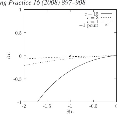
The corresponding Nyquist diagram appears in figure 4 for three values of damping
constant c. It is a fundamental result that connecting two passive systems by energy
ports yields a stable system, so it is unsurprising that as revealed by figure 4 the
loop-gain has a positive phase margin for each value of c. The numerical values of
the phase-marginθmappears in table 1 for each value of c.
However, and this is the key point, the phase-margin is very small for small
val-ues of c. Again, this is unsurprising as this small phase margin is precisely what
is required to give a sharp resonance in the overall AbHWiL system of figure 3.
This small phase margin gives rise to the extreme sensitivity problem discussed
elsewhere (Gawthrop et al., 2005b, 2006; Wallace et al., 2005b); in particular, a
Control Engineering Practice 16 (2008) 897–908
instability. As discussed by Gawthrop et al. (2006), robust stability can be obtained
at the expense of fidelity by appropriate control design. However, the main thrust of
this paper is to remove the transfer system as accurately as possible thus giving
ac-curate fidelity despite the small phase margin. Nevertheless, the issue of robustness
is still crucial and so is analysed further here in the context of EBC.
4.3 Robustness
As mentioned in§3, the fact that the nominal system of figure 2(b) is replaced by
the emulator-based system of figure 2(c) means that the analysis is different. In
particular, the expression for the loop-gain is no longer given by (31). The actual
loop gain is now derived. With reference to figure 2(c), the transfer function Na(s)
of the augmented software subsystem relating y(s)to−u(s)is:
Na(s) =− y(s)
u(s) =
N(s) 1+N(s)CG((ss))
F(s)
C(s) =
BN(s)F(s) AN(s)C(s) +BN(s)G(s)
(34)
For analysis purposes the following assumption is required:
Assumption 4 Na(s)is stable.
It is part of the EBC design process to ensure that assumption 4 holds. The loop
gain L(s)corresponding to figure 2(c) is thus:
L(s) =Na(s)T(s)P(s) =e−sτ
BT(s)BN(s)BP(s)H(s)
AP(s)(AN(s)C(s) +BN(s)BP(s)E(s))
(35)
Equation (35) is now used to investigate the robustness of the EBC to errors in
modelling the physical system P(s).
Control Engineering Practice 16 (2008) 897–908
The hardware component of the AbHWiL system has, thus far, been taken to be
a known linear system with transfer function P(s). However, such a model may
not be accurate and thus it is important to investigate the robustness of the EBC
approach in the presence of such inaccuracy. To do this, assume that the physical
system comprises the nominal system P(s)in series with a neglected system ˜P. Two
stability theorems are given: one for linear time invariant ˜P and one for memoryless
nonlinearities.
Theorem 1 Given assumptions 1– 4, if ˜P is a stable, linear, time-invariant system
with transfer function ˜P(s) and if the frequency locus ˜P(s)L(s) does not encircle
the -1 point in the complex plane as s traverses the Nyquist D contour, then the
perturbed closed-loop system is stable.
PROOF. This is a restatement of Nyquist’s theorem (Goodwin et al., 2001; Nyquist,
1932) for stable open-loop systems. 2
Theorem 2 Given assumptions 1– 4, if ˜P=P˜(z)is a memoryless, sector-bounded
non-linearity where for someα>0
1−α< P˜(z)
z <1+α ∀z6=0 (36)
and if the frequency locus L(s)does not encircle the -1 point in the complex plane
as s traverses the Nyquist D contour and the locus does not intersect the circle in
the complex plane centred at 1−1α2 with radius 1−αα2, then the system is uniformly
asymptotically stable.
Control Engineering Practice 16 (2008) 897–908
In addition to stability, it would be interesting to obtain bounds on the error caused
by such nonlinearities; this is a matter for future research.
5 Experimental Investigation
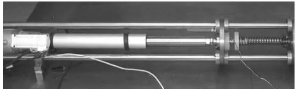
[Fig. 6 about here.]
The AbHWiL system of figure 3 was experimentally investigated in four stages:
identification of the transfer system transfer function T(s), design of the
corre-sponding EBC, robustness analysis and experimental results.
The experimental setup of figure 6 consists of a spring - the hardware component
- connected, via a load cell, to an electro-mechanical ball-screw actuator. This
ac-tuator is driven by a proprietary controller; in proportional displacement control.
In RTDS literature the proprietary controller is often referred to as the inner-loop
controller to distinguish it from the outer-loop control strategy; the EBC in the
im-plementation considered here. The transfer system, T(s), consists of both the
inner-loop controller and the actuator. Since the EBC strategy operates in velocity control
and the inner-loop controller operates in displacement control the EBC control
sig-nal is integrated before being sent as the demand sigsig-nal to the inner-loop controller.
The software model, along with the EBC strategy was written in Matlab-Simulink
Control Engineering Practice 16 (2008) 897–908 5.1 Transfer system identification
The response of the transfer system T(s)was measured experimentally by applying
a square wave displacement setpoint to the transfer system controller; and the
cor-responding displacement was measured. The second order with delay model of the
form ˆT(s) =e−sτ kt
mts2+cts+kt was used; this is a special case of (5) where BT(s) =1.
[image:21.595.94.489.499.653.2]Using an optimisation approach (Gawthrop, 2000; Ljung, 1999), the parameters in
Table 2 were found to give a good fit.
5.2 Emulator design
It is convenient to work in a normalised time scale with a time unit of 10ms. With
these time units,τ=0.5 and T(s) = 0.59656s2+01.51792s+1 The hardware component
P(s) (32) is first order and so, using (12) the equivalent system has a third order
denominator. Using design rule 2 choose C(s)second order; in particular (in this
time-scale) choose
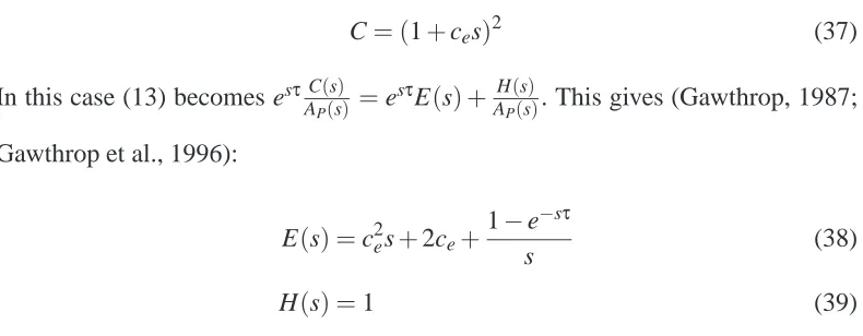
C= (1+ces)2 (37)
In this case (13) becomes esτAC(s)
P(s) =e
sτE(s) + H(s)
AP(s). This gives (Gawthrop, 1987;
Gawthrop et al., 1996):
E(s) =c2es+2ce+
1−e−sτ
s (38)
H(s) =1 (39)
As mentioned in §3, (38) has two problems: it contains an irrational term and it
contains an implicit cancellation of s. Both can be overcome by approximating the
Control Engineering Practice 16 (2008) 897–908
table 3.1)
e−sτ≈ 1−
sτ 2 +
(sτ)2
12
1+12sτ+(s12τ)2
(40)
This approximation is adequate over the frequency range of interest. It follows that:
1−e−sτ
s ≈
τ
1+12sτ+(s12τ)2
(41)
Thus
G(s)
C(s) =
E(s)B(s)
C(s) ≈ks
(c2es+2ce)(1+12sτ+(sτ) 2
12 ) +τ
(ces+1)2(1+12sτ+(sτ) 2
12 )
(42)
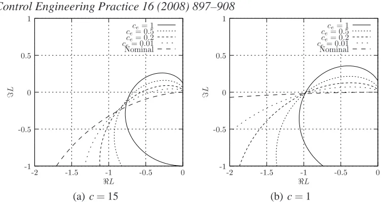
5.3 Robustness analysis
[Fig. 7 about here.]
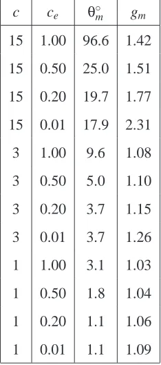
Figures 7(a)–7(b) show the Nyquist diagrams for three cases of software system
damping c=15 and c=1. In each case, the diagram is plotted for choices of the
emulator polynomial C(s)(37): ce=1,0.5,0.2,0.01 and, for comparison, the
nom-inal loop-gain of figure 4. Table 3 gives the corresponding phase and gain margins.
Comparing tables 3 and 1 (the case as ce →0), it can be seen that increasing ce
increases the phase margin and thus increases robustness to small phase errors in
T(s). On the other hand, both figure 7 and table 3 indicate that increasing ce
de-creases the gain margin and thus dede-creases robustness with respect to uncertainty
in ks. In each case, the small stability margins indicate the demanding nature of the
Control Engineering Practice 16 (2008) 897–908 5.4 Experimental results
A number of experiments were conducted using the apparatus of §5 5.1 , and the
EBC designed in §5 5.2 . These can be divided into two categories, sinusoidal tests
where
r(s) =Aisin(2πfit+θi) (43)
and multi-sine test where
r(s) =
N
∑
i=1
Aisin(2πfit+θi) (44)
[Fig. 8 about here.]
Sinusoidal tests (43) were carried out for frequencies fi=3,4,5,6,8,9,10Hz (43),
three values of damping c as listed in figure 3, and two values of emulator constant
ce=0.2,0.5 (37). A signal at 7Hz was omitted as the equipment cannot cope with
signals near to the resonance at 7.2Hz. In each case, the measured values of y=F
(the spring force measured by the load cell), reference signal r, x (measured transfer
system displacement) were recorded every msec for about 5sec. For the purposes of
computing the properties of the sinusoid, the data was truncated to give an integer
number of periods.
Perhaps the most striking result is qualitative; the EBC was stable even at the low
damping (c=1). In contrast, it was not possible to stabilise this system below c=3
using the predictive method reported previously (Wallace et al., 2005b).
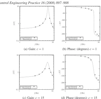
The relative gain g and phaseφof the sinusoidal signals x and r was computed and
compared with those computed from X(s)T(s)(28) using the parameter values of
Control Engineering Practice 16 (2008) 897–908
and smallest (c=1) damping coefficients and for emulator parameter ce =0.2;
the results for c= 5 and ce =0.5 are similar and not shown. In each case, the
experimental and theoretical gains are closely matched indicating good fidelity of
the EBC; the phases are not in such good agreement. Further experimental
inves-tigation revealed that the spring could be more accurately modelled by including
structural damping to give the dynamic spring constant K(s)
K(s) =ks+css (45)
where the estimated damping was cs=3Nsm−1and that this explained some of the
phase error. This is an example of a linear ˜P=1+cs
kss as discussed in §4 4.3 .
[Fig. 9 about here.]
To demonstrate the behaviour of EBC when using non-sinusoidal signals, a
multi-sine reference r was constructed from (44) using the frequencies of figure 8.
Fig-ure 9 shows typical 2sec sequences of desired x0 and actual x displacements for
the same controller parameters used in figure 8. The close match between desired
and experimental displacements verifies that the method is appropriate to
non-sinusoidal reference signals such as a typical earthquake signal.
It was noted that for small values of input (not shown), the experimental response
was dominated by a stable limit cycle at a frequency of about 7Hz; this limit cycle
disappeared as the signal levels were increased to the values shown in Figure 9.
As the measured displacement showed signs of stiction, we suspect the presence
of “friction generated limit cycles” (Olsson & ˚Astr¨om, 2001) due to ball-screw
Control Engineering Practice 16 (2008) 897–908 6 Conclusion
Emulator based control is a well-established controller design method. In this paper
we have shown how it can be used to provide a novel but natural way of
remov-ing the unwanted transfer system dynamics from an AbHWiL test. In fact this
ap-proach gives a significant improvement in control fidelity over previous methods,
as we have demonstrated with the example system considered in this paper. The
main advantages are; (i) more complex forms of transfer system dynamics can be
compensated for, leading to improved fidelity and stability, (ii) the correct gain and
phase compensation are applied at any frequency, without the need for adaption,
(iii) multi-frequency signals can be dealt with, and (iv) there is a preexisting
robust-ness theory to guide the choice of design parameters. Unlike previous approaches
using Smith’s predictor, the method presented here is not restricted to stable
tems with well-damped resonances — a critical feature for AbHWiL/RTDS
sys-tems with lightly damped resonances. In fact emulator based control has a further
advantage over Smith’s predictor in that it removes unwanted dynamics described
by a rational transfer function as well as those described by a pure time-delay.
To achieve these advantages over previous RTDS approaches, we have exploited
the fact that for many applications an approximate linear model of the critical
com-ponent will be available. The emulator based control is then able to cope with the
subsequent under-modelled nonlinearities (and other uncertainties) by using robust
nonlinear control techniques, as we have demonstrated by application of the circle
criterion. For systems without a linear plant model, or with nonlinearities which do
Control Engineering Practice 16 (2008) 897–908
would not be appropriate. An area of future research is to use adaptive emulator
approach (in fact there is already a large literature containing not only algorithms
but adaptive robustness results for emulator based self-tuning controllers) to allow
a wider class of nonlinear critical components to be included.
Acknowledgements
Peter Gawthrop is a Visiting Research Fellow at Bristol University. The other
au-thors would like to acknowledge the support of the EPSRC: David Virden is
sup-ported by EPSRC grant (GR/R99539/01) and David Wagg via an Advanced
Re-search Fellowship.
References
˚
Astr¨om, K. J. 1970. Introduction to Stochastic Control Theory. Academic Press,
New York.
˚
Astr¨om,K. J. & Wittenmark,B. 1973. On self-tuning regulators. Automatica, 9:
185–199.
Agrawal,A.K. & Yang,J.N. 2000. Compensation of time-delay for control of civil
engineering structures. Earthquake Engng Struc. Dyn., 29(1):37–62.
Blakeborough, A., Williams, M.S., Darby, A.P. & Williams, D.M. 2001. The
de-velopment of real-time substructure testing. Philosophical Transactions of the
Royal Society pt. A, 359(1869-1891).
automatic-Control Engineering Practice 16 (2008) 897–908
transmission control units in the form of hardware-in-the-loop. Internationa
Journal of Vehicle Design, 28:(84-102).
de Carufel, J., Martin, E. & Piedboeuf, J. C. 2000. Control strategies for
hardware-in-the-loop simulation of flexible space robots. IEE Proceedings-Control Theory
and Applications, 147:569–579.
Clarke,D. W. & Gawthrop, P. J. 1975. Self-tuning controller. IEE Proceedings
Part D: Control Theory and Applications, 122(9):929–934.
Darby,A.P., Williams,M.S., & Blakeborough, A. 2002. Stability and delay
com-pensation for real-time substructure testing. ASCE Journal of Engineering
Me-chanics, 128:1276–1284.
Driscoll, S.; Huggins, J.D. & Book, W.J. 2005. Electric Motors Coupled to
Hy-draulic Motors as Actuators for HyHy-draulic Hardware-in-the-Loop Simulation.
Proceedings of ASME International Mechanical Engineering Congress and
Ex-position, paper IMECE2005-82124.
Faithfull, P. T., Ball, R. J. & Jones, R. P. 2001. An investigation into the use of
hardware-in-the-loop simulation with a scaled physical prototype as an aid to
design. Journal of Engineering Design, 12:231–243.
Fathy, H.K.; Ahlawat, R. & Stein, J.L. 2006. Proper Powertrain Modeling for
Engine-in-the-Loop Simulation. Proceedings of the ASME International
Engi-neering Congress and Exposition, paper IMECE2005-81592.
Ferreira, J. A., Almeida, F. G., Quintas, M. R. & de Oliveira, J. P. E. 2004. Hybrid
models for hardware-in-the-loop simulation of hydraulic systems Part 2:
experi-ments. Proceedings of the Institution of Mechanical Engineers Part I-Journal of
Systems and Control Engineering, 218:475–486.
Control Engineering Practice 16 (2008) 897–908
models for hardware-in-the-loop simulation of hydraulic systems Part 1: theory.
Proceedings of the Institution of Mechanical Engineers Part I-Journal of Systems
and Control Engineering, 218:465–474.
Ganguli, A., Deraemaeker, A., Horodinca, M. & Preumont, A. 2005. Active
damp-ing of chatter in machine toolsdemonstration with a ’hardware-in-the-loop’
sim-ulator. Proceedings of the Institution of Mechanical Engineers Part I-Journal of
Systems and Control Engineering, 219:359–369.
Gawthrop, P. J. 1987. Continuous-time Self-tuning Control. Vol 1: Design.
Re-search Studies Press, Engineering control series., Lechworth, England.
Gawthrop,P. J., Jones, R. W., & Sbarbaro, D. G. 1996. Emulator-based control
and internal model control: Complementary approaches to robust control design.
Automatica, 32(8):1223–1227.
Gawthrop., P.J. 2000. Sensitivity bond graphs. Journal of the Franklin Institute,
337(7):907–922.
Gawthrop., P.J. 2004. Bond graph based control using virtual actuators.
Proceed-ings of the Institution of Mechanical Engineers Pt. I: Journal of Systems and
Control Engineering, 218(4):251–268.
Gawthrop, P.J. 2005. Virtual actuators with virtual sensors. Proceedings of the
Institution of Mechanical Engineers Pt. I: Journal of Systems and Control
Engi-neering, 219(5):371 – 377.
Gawthrop,P.J., Wallace,M.I. & Wagg, D.J. 2005b. Bond-graph based substructuring
of dynamical systems. Earthquake Engng Struc. Dyn., 34(6):687–703.
Gawthrop,P.J.,Wallace, M.I., Neild, S.A. & Wagg, D.J. 2006. Robust real-time
substructuring techniques for under-damped systems. Structural Control and
Control Engineering Practice 16 (2008) 897–908
G.C. Goodwin, S.F. Graebe, & M.E. Salgado. Control System Design. Prentice
Hall, 2001.
Hong, K. S., Sohn, H. C. & Hedrick, J. K. 2002. Modified skyhook control of
semi-active suspensions: A new model, gain scheduling, and hardware-in-the-loop
tuning. Journal of Dynamic Systems Measurement and Control-Transactions
of the ASME, 12400158–167.
Horiuchi,T. & Konno,T. 2001. A new method for compensating actuator delay in
real-time hybrid experiments. Philisophical Transactions of the Royal Society,
Pt.A, 359:1893–1909.
Horiuchi, T., Inoue, M., Konno, T. & Namita, Y. 1999. Real-time hybrid
experi-mental system with actuator delay compensation and its application to a piping
system with energy absorber. Earthquake Engng Struc. Dyn., 28:1121–1141.
Jezernik, S. 2005. Hardware-in-the-loop simulation and analysis of magnetic
recording of nerve activity. Journal of Neuroscience Methods, 142:295–304.
Lambrechts, P., Boerlage, M. & Steinbuch, M. 2005. Trajectory planning and
feedforward design for electromechanical motion systems. Control
Engineer-ing Practice, 13:145–157.
Ljung,L. 1999. System Identification: Theory for the User. Information and
Sys-tems Science. Prentice-Hall, 2nd edition.
MacLane, S. & Birkhoff, G. 1967. Algebra. Macmillan, New York.
Mansoor, S. P., Jones, D. I., Bradley, D. A., Aris, F. C. & Jones, G. R. 2003.
Hardware-in-the-loop simulation of a pumped storage hydro station.
Interna-tional Jornal of Power and Energy Systems, 23:127–133.
Marshall, J. E. 1979. Control of Time-delay Systems. Peter Peregrinus.
Control Engineering Practice 16 (2008) 897–908
time delay compensation in active structural control. In Proceedings of the 6th
International Modal Analysis Conference-IMAC, volume 1, pages 733–739.
Misselhorn, W. E., Theron, N. J. & Els, P. S. 2006. Investigation of
hardware-in-the-loop for use in suspension development. Vehicle System Dynamics, 44:
65–81.
Morari, M. & Zafiriou, E. 1989. Robust Process Control. Prentice-Hall, Englewood
Cliffs.
Nyquist, H. 1932. Regeneration theory. Bell Syst. Tech. J., 11:126–147.
Olsson, H. & ˚Astr¨om, K.J. 2001. Friction generated limit cycles. Control Systems
Technology, IEEE Transactions on, 9(4):629–636.
Plummer, A. R. 2006. Model-in-the-loop testing. Proc IMechE Part I-Journal of
Systems and Control Engineering, 220:183–199.
Reinhorn, A.M. , Sivaselvan, M.V., Liang, Z., & Shao, X. 2004. Real-time
dy-namic hybrid testing of structural systems. In Thirteenth World Conference on
Earthquake Engineering, Vancouver. Paper No 1644.
Rulka, W. & Pankiewicz, E. 2005. MBS approach to generate equations of motions
for HiL-simulations in vehicle dynamics. Multibody system dynamics, 14:367–
386.
Smith, O. J. M. 1959. A controller to overcome dead-time. ISA Transactions, 6(2):
28–33.
Wagg, D.J. & Stoten, D.P. 2001. Substructuring of dynamical systems via the
adaptive minimal control approach. Earthquake Engng Struc. Dyn., 30(6):865–
877.
Wallace, M.I., Sieber, J., Neild, S.A., Wagg, D.J. & Krauskopf, B. 2005a. A delay
Control Engineering Practice 16 (2008) 897–908 Engng Struc. Dyn., 34(15):1817 – 1832.
Wallace, M.I., Wagg, D.J. & Neild, S.A. 2005b. An adaptive polynomial based
for-ward prediction algorithm for multi-actuator real-time dynamic substructuring.
Proceedings of the Royal Society, 461(2064):3807 – 3826.
Willems, J. C., 1972. Dissipative dynamical systems, part I: General theory, part
II: Linear system with quadratic supply rates. Arch. Rational Mechanics and
Analysis, 45:321–392.
Williams, M.S. & Blakeborough, A. 2001. Laboratory testing of structures under
dynamic loads: an introductory review. Philosophical Transactions of the Royal
Society, 359:1651–1669.
Zames, G. 1966a. On the input-output stability of time-varying nonlinear systems
– part I: Conditions derived using concepts of loop gain, conicity and positivity.
IEEE Trans. on Automatic Control, 11(2):228–238.
Zames, G. 1966b. On the input-output stability of time-varying nonlinear systems
– part II: Conditions involving circles in the frequency plane and sector
nonlin-earities. IEEE Trans. on Automatic Control, 11(3):465–476.
Zhang, R. & Alleyne, A. G. 2005. Dynamic emulation using an indirect control
input. Journal of Dynamic Systems Measurement and Control - Transactions of
the ASME, 127:114–124.
Zhu, W. D., Pekarek, S., Jatskevich, J., Wasynczuk, O. & Delisle, D. 2005. A
model-in-the-loop interface to emulate source dynamics in a zonal DC
distribu-tion system. IEEE Transacdistribu-tions on Power Electronics, 20:438–445.
[Table 1 about here.]
Control Engineering Practice 16 (2008) 897–908
Control Engineering Practice 16 (2008) 897–908 List of Figures
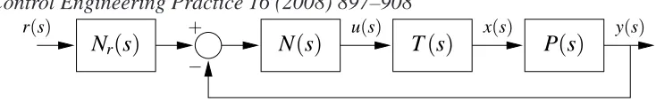
1 Substructuring as a feedback system. P(s)is the hardware component transfer function, N(s)and Nr(s)are the software substructure transfer functions and T(s)is the transfer system
transfer function. 33
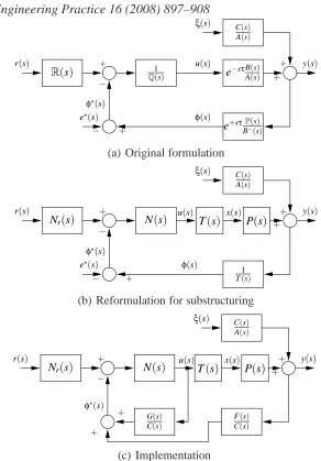
2 Emulator-based control. (a) shows the general EBC formulation of Gawthrop (1987). (b) shows the particular form appropriate to substructuring which appears to cancel T(s). (c) shows the
approximate, but realisable, implementation of (b). 34
3 An AbHWiL system. The physical system, comprising a mass, two springs and a damper, is configured so that the spring ks is the hardware component; the other components form the software subsystem. r is the imposed wall displacement. The numerical values used are: c=1,3 or 15Nm−1s, k=ks=2250Nm−1 and
m=2.2kg 35
4 Nominal loop gain. L0(s)(31) is plotted for three values of
damping coefficient: c=15,3,1 36
5 Robustness analysis. The physical system has been split into a
nominal part P(s)and neglected part ˜P 37
6 Experimental Equipment. The hardware component (spring) lies to the right, the transfer system (actuator) is the linear
electro-mechanical transducer at the left. 38
7 Actual loop-gain. (a) L(s)(35), with damping coefficient c=15, is plotted for five values of damping coefficient: ce=1,0.5,0.2,0.01 and c=1 as well as for the nominal loop gain L0(s)(31) of figure
4. (b) is as (a) except that the damping coefficient c=1; the
stability margins are smaller in this case. 39
8 Frequency response. Experimental points marked with ×are
superimposed on theoretical frequency response of T(s)X(s)(28). 40
9 Multi-sine tests. The reference signal is a weighted sum of sinusoids at 3,4,5,6,8,9&10Hz with amplitude adjusted to give
Control Engineering Practice 16 (2008) 897–908
Nr
(
s
)
N
(
s
)
T
(
s
)
P
(
s
)
y(s)r(s)
−
[image:34.595.98.465.77.134.2]+ u(s) x(s)
Control Engineering Practice 16 (2008) 897–908
e−sτB(s)
A(s)
1
Q(s)
C(s)
A(s)
e+sτP(s)
B−(s)
R(s)
ξ(s)
r(s) u(s) y(s)
+
−
+ +
φ⋆(s)
e⋆(s) φ(s)
− +
(a) Original formulation
N(s)
C(s)
A(s)
1
T(s)
Nr(s) T(s) P(s)
ξ(s)
r(s) y(s)
+
−
+ +
φ⋆(
s)
u(s)
e⋆(s) φ(s)
− +
x(s)
(b) Reformulation for substructuring
N(s)
C(s)
A(s)
Nr(s) T(s)
F(s)
C(s)
G(s)
C(s)
P(s) ξ(s)
r(s) y(s)
+ − + + + + φ⋆(s)
u(s) x(s)
[image:35.595.138.430.70.489.2](c) Implementation
Control Engineering Practice 16 (2008) 897–908
m k
c
r ks
Control Engineering Practice 16 (2008) 897–908
-1 -0.5 0 0.5 1
-2 -1.5 -1 -0.5 0
ℑ
L
ℜL
[image:37.595.179.384.74.276.2]c= 15 c= 3 c= 1 −1point
Fig. 4. Nominal loop gain. L0(s) (31) is plotted for three values of damping coefficient:
Control Engineering Practice 16 (2008) 897–908
Na(s)
C(s)
A(s)
T(s) P(s)
Nar(s)
˜
P
ξ(s)
r(s) y0(s)
+ −
+ +
y(s)
[image:38.595.113.406.71.185.2]u(s) x(s)
Fig. 5. Robustness analysis. The physical system has been split into a nominal part P(s)
Control Engineering Practice 16 (2008) 897–908
Control Engineering Practice 16 (2008) 897–908
-1 -0.5 0 0.5 1
-2 -1.5 -1 -0.5 0
ℑ
L
ℜL
ce= 1
ce= 0.5
ce= 0.2
ce= 0.01 Nominal
(a) c=15
-1 -0.5 0 0.5 1
-2 -1.5 -1 -0.5 0
ℑ
L
ℜL
ce= 1
ce= 0.5
ce= 0.2
ce= 0.01 Nominal
[image:40.595.97.474.72.272.2](b) c=1
Fig. 7. Actual loop-gain. (a) L(s)(35), with damping coefficient c=15, is plotted for five values of damping coefficient: ce =1,0.5,0.2,0.01 and c=1 as well as for the nominal loop gain L0(s)(31) of figure 4. (b) is as (a) except that the damping coefficient c=1; the
Control Engineering Practice 16 (2008) 897–908 0.1 1 10 1 10 | X T | f(Hz) experimental theoretial
(a) Gain: c=1
-250 -200 -150 -100 -50 0 1 10 6X T f(Hz) experimental theoretial
(b) Phase: (degrees) c=1
0.1 1 10 1 10 | X T | f(Hz) experimental theoretial
(c) Gain: c=15
-250 -200 -150 -100 -50 0 1 10 6X T f(Hz) experimental theoretial
[image:41.595.100.437.69.398.2](d) Phase (degrees): c=15
Control Engineering Practice 16 (2008) 897–908
-15 -10 -5 0 5 10 15
0 0.2 0.4 0.6 0.8 1 1.2 1.4 1.6 1.8 2
x
(mm)
t(se)
x x0
(a) c=1
-15 -10 -5 0 5 10 15
0 0.2 0.4 0.6 0.8 1 1.2 1.4 1.6 1.8 2
x
(mm)
t(se)
x x0
[image:42.595.101.474.71.214.2](b) c=15
Control Engineering Practice 16 (2008) 897–908 List of Tables
1 Nominal phase-margin: c=15,3,1 43
2 Estimated transfer system parameters 44
Control Engineering Practice 16 (2008) 897–908
c θ◦m
15 17.3
3 3.5
1 1.1
Table 1
Control Engineering Practice 16 (2008) 897–908
Parameter Value
ct 191Nm−1s kt 36878Nm−1
mt 2.2kg
Table 2
Control Engineering Practice 16 (2008) 897–908
c ce θ◦m gm
15 1.00 96.6 1.42
15 0.50 25.0 1.51
15 0.20 19.7 1.77
15 0.01 17.9 2.31
3 1.00 9.6 1.08
3 0.50 5.0 1.10
3 0.20 3.7 1.15
3 0.01 3.7 1.26
1 1.00 3.1 1.03
1 0.50 1.8 1.04
1 0.20 1.1 1.06
[image:46.595.231.348.267.531.2]1 0.01 1.1 1.09 Table 3