Event-Triggered Consensus and Formation Control in Multi-Agent Coordination

Formation Control in Multi-Agent

Coordination

Qingchen Liu

A thesis submitted for the degree of

Doctor of Philosophy

The Australian National University

My doctoral studies have been conducted under the guidance and supervision of Assoc. Prof. Changbin (Brad) Yu, Dr. Jonghyuk Kim and Prof. Jiahu Qin. This thesis contains no material which has been accepted for the award of any other degree or diploma in any university.

Most of the results in this thesis have been published at refereed international journals or international conferences. Some of these results have been achieved in collaboration with other researchers. Co-authored publications as a result of parts of my thesis research are listed as below:

Refereed Journal Papers

1. Z. Sun,Q. Liu, C. Yu and B. D. O. Anderson. Cooperative Event-Based Rigid Formation Control. In revision, to be submitted to IEEE Transactions on Net-work Science and Engineering.

2. Q. Liu, M. Ye, J. Qin and C. Yu. Event-Triggered Algorithms for Leader-Follower Consensus of Networked Euler-Lagrange Agents. Accepted by IEEE Transaction on Systems, Man and Cybernetics: Systems.

3. Q. Liu, J. Qin and C. Yu. Event-based Agreement Protocols for Complex Net-works with Time Delays under Pinning Control. Journal of The Franklin Insti-tute, vol. 353, no. 15, pp. 3999-4015, 2016.

Refereed Conference Papers

4. P. Fang,Q. Liu, X. Hou, J. Qin and C. Yu. Edge-Event-Based Multi-Agent Con-sensus with Zeno-free Triggers under Synchronized/Unsynchronized Clocks. Accepted, to be presented at the 56th IEEE Conference on Decision and Con-trol (CDC’17), Melbourne, Australia, 2017.

5. Q. Liu, M. Ye, Z. Sun, J. Qin and C. Yu. Coverage Control of Unicycle Agents under Constant Speed Constraints. Proc. of the 20th IFAC World Congress (IFAC WC’17), pp. , Toulouse, France, 2017.

6. C. Huang,Q. Liuand C. Yu. Uniform Upper Bound of the Spectrum of Rooted Graphs. Proc. of the Australian Control Conference (AUCC’16), pp. 105-109, Newcastle, Australia, 2016.

7. Q. Liu, M. Ye, J. Qin and C. Yu. Event-Based Leader-Follower Consensus for Multiple Euler-Lagrange Systems with Parametric Uncertainties. Proc. of the

8. Q. Liu, J. Qin and C. Yu. Event-Based Multi-Agent Cooperative Control with Quantized Relative State Measurements. Proc. of the 55th IEEE conference of Decision and Control (CDC’16), pp. 2240-2246, Las Vegas, USA, 2016.

9. Q. Liu, Z. Sun, J. Qin and C. Yu. Distance-Based Formation Shape Stabilization via Event-Triggered Control. Proc. of the 34th Chinese Control Conference (CCC’15), pp. 6948-6953, Hangzhou, China, 2015.

Firstly and foremost, I would like to express my sincere gratitude to my principal supervisor, Assoc. Prof. Changbin (Brad) Yu, who has been incredibly supportive since I first met him. I was recruited by Brad in Shandong Computer Science Center (SCSC) in late 2012 as a team member under his leadership. This precious opportu-nity to work with a young, creative researcher from a world-leading group benefits me a lot from various perspectives. At this stage, Brad also provides me a lot of support in my PhD application and suggestions in the future research directions, which paved a smooth way for me to start a PhD journey at ANU. In my four years life at ANU, Brad endowed me lots of freedom to explore the research topics of my own interest and offer me invaluable discussions on these topics. He also provides me great opportunities to attend international conferences so that I can get in touch with cutting-edge research topics and discuss with worldwide researchers. Besides research, Brad would also like to share his life experience with me in our numerous hot pot "banquets", which brings me more insights on different aspects of lives.

Secondly, I would also like to thank my co-supervisor, Prof. Jiahu Qin, for his great help and support in my research journey. During these four years, he would always like to sacrifice his time to discuss with me on my research topics or answer my questions, no matter how busy he was. We had discussions at midnights, at the time he was at airports or train stations. My training as a research student would not be complete without his guidance. Jiahu’s life attitude also affects me a lot, from which I learnt how a researcher balances his time between work and family.

Thirdly, I would like to thank my friends and colleagues, Dr. Zhiyong Sun and Mr. Mengbin Ye, for sharing their knowledges with me. I started to work with Zhiyong in SCSC and have always received his great help since that. Zhiyong is the person who inspired me to find my PhD research direction: distributed event-triggered control for multi-agent systems. He would always like to share his research experience with me and help me at all the aspects in research. Mengbin is my best partner in research. His cautious attitude to work really benefits me a lot.

I also take this opportunity to thank Dr. Jonghyuk Kim, for his kind help and suggestions during my PhD study and Prof. Brian D.O. Anderson, for his invaluable comments to my research papers. I would also thank Prof. Sandra Hirche, for hosting me as a visiting student in her group where I gained different insights to my research topics by interacting with a robotic researcher.

My time as a PhD student at ANU is with so much happiness by interacting with many nice friends. They are Dr. Yun (Gavin) Hou, Dr. Xiaolei (Eric) Hou, Dr. Junming (Jamie) Wei, Dr Yiming Ji, Yonhon Ng, Pengfei Fang, Dr. Chao Huang, Dr. Yinqiu Wang, Dr. Pan Ji, Dr. Gao Zhu, Yaoxian Song, Zhixun Li at ANU, Dr. Na

My PhD research has been supported by an ANU-CSC scholarship awarded jointly by ANU and China Scholarship Council. The financial support from this scholarship is greatly appreciated. I am also thankful to Mr. Linlan Ma, who is a secretary in the education office of China Embassy in Australia, for his kind help in dealing with various issues regarding my scholarship.

The focus of this thesis is to study distributed event-triggered control for multi-agent systems (MASs) facing constraints in practical applications. We consider sev-eral problems in the field, ranging from event-triggered consensus with information quantization, event-triggered edge agreement under synchronized/unsynchronized clocks, event-triggered leader-follower consensus with Euler-Lagrange agent dynam-ics and cooperative event-triggered rigid formation control.

The first topic is named as event-triggered consensus with quantized relative state measurements. In this topic, we develop two event-triggered controllers with quan-tized relative state measurements to achieve consensus for an undirected network where each agent is modelled by single integrator dynamics. Both uniform and log-arithmic quantizers are considered, which, together with two different controllers, yield four cases of study in this topic. The quantized information is used to up-date the control input as well as to determine the next trigger event. We show that approximate consensus can be achieved by the proposed algorithms and Zeno be-haviour can be completely excluded if constant offsets with some computable lower bounds are added to the trigger conditions.

The second topic considers event-triggered edge agreement problems. Two cases, namely the synchronized clock case and the unsynchronized clock case, are studied. In the synchronized clock case, all agents are activated simultaneously to measure the relative state information over edge links under a global clock. Edge events are defined and their occurrences trigger the update of control inputs for the two agents sharing the link. We show that average consensus can be achieved with our proposed algorithm. In the unsynchronized clock case, each agent executes control algorithms under its own clock which is not synchronized with other agents’ clocks. An edge event only triggers control input update for an individual agent. It is shown that all agents will reach consensus in a totally asynchronous manner.

In the third topic, we propose three different distributed event-triggered con-trol algorithms to achieve leader-follower consensus for a network of Euler-Lagrange agents. We firstly propose two model-independent algorithms for a subclass of Euler-Lagrange agents without the vector of gravitational potential forces. A variable-gain algorithm is employed when the sensing graph is undirected; algorithm parameters are selected in a fully distributed manner with much greater flexibility compared to all previous work concerning event-triggered consensus problems. When the sensing graph is directed, a constant-gain algorithm is employed. The control gains must be centrally designed to exceed several lower bounding inequalities which require lim-ited knowledge of bounds on the matrices describing the agent dynamics, bounds on network topology information and bounds on the initial conditions. When the Euler-Lagrange agents have dynamics which include the vector of gravitational potential

forces, an adaptive algorithm is proposed. This requires more information about the agent dynamics but allows for the estimation of uncertain agent parameters.

Declaration vii

Acknowledgments ix

Abstract xi

1 Introduction 1

1.1 Research background . . . 1

1.2 Contributions and Outline . . . 3

2 Preliminary 7 2.1 Notations . . . 7

2.2 Event-triggered consensus: a revisit . . . 7

2.2.1 The consensus problem . . . 7

2.2.2 Basic trigger schemes . . . 11

2.2.2.1 Self-measurement-based scheme . . . 11

2.2.2.2 Edge-measurement-based scheme . . . 14

2.2.2.3 Local-measurement-based scheme . . . 15

2.2.3 Zeno behaviour . . . 18

2.2.4 Zeno-free approaches . . . 20

2.2.4.1 Time-dependent trigger function . . . 20

2.2.4.2 Static trigger function . . . 22

2.2.4.3 Time-regulation trigger condition . . . 23

2.3 Chapter summary . . . 24

3 Event-Triggered Consensus with Quantized Relative Information 25 3.1 Introduction . . . 25

3.2 Additional Preliminaries . . . 26

3.2.1 Quantizer functions . . . 26

3.2.2 Quantizer properties . . . 26

3.3 Problem formulation . . . 27

3.4 Input quantization case . . . 28

3.5 Edge quantization case . . . 32

3.6 Simulation examples . . . 36

4 Edge-Event-Triggered Consensus under Synchronized and Unsynchronized

Clocks 41

4.1 Introduction . . . 41

4.1.1 Problem formulation . . . 42

4.2 Synchronized clock case . . . 43

4.3 Unsynchronized clock case . . . 46

4.4 Simulation examples . . . 50

4.5 Concluding remarks . . . 51

5 Event-Triggered Consensus for Networked Euler-Lagrange Agents 53 5.1 Introduction . . . 53

5.2 Additional preliminaries . . . 54

5.2.1 Graph theory . . . 56

5.2.2 Euler-Lagrange systems . . . 57

5.3 Problem statement . . . 58

5.4 Variable-gain, model-independent algorithm . . . 58

5.4.1 Main result . . . 59

5.4.1.1 Stability analysis . . . 61

5.4.1.2 Absence of Zeno behaviour . . . 64

5.4.2 Discussions on the choice of trigger functions . . . 66

5.4.2.1 SDTF . . . 67

5.4.2.2 TDTF . . . 67

5.4.2.3 MTF . . . 70

5.5 Fixed gain, model-independent algorithm . . . 71

5.5.1 An upper bound using initial conditions . . . 74

5.5.2 Main proof . . . 75

5.6 Adaptive, model-dependent algorithm . . . 81

5.6.1 Main result . . . 81

5.7 Simulations . . . 85

5.8 Concluding remarks . . . 89

6 Event-Triggered Rigid Formation Control 91 6.1 Introduction . . . 91

6.2 Preliminaries . . . 92

6.2.1 Basic concepts on rigidity theory . . . 92

6.2.2 Problem statement . . . 94

6.3 Centralized control algorithm . . . 94

6.3.1 Centralized algorithm design . . . 95

6.3.2 Exclusion of Zeno behaviour . . . 98

6.4 Distributed control algorithm . . . 101

6.4.1 Distributed algorithm design . . . 101

6.4.2 Trigger behaviour analysis . . . 104

6.4.3 A modified distributed trigger function . . . 105

6.6 Concluding remarks . . . 110

7 Conclusions 113

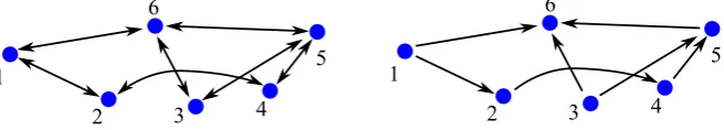
2.1 Left: An undirected graph. Right: A corresponding directed graph with arbitrarily chosen edge orientations for constructing the incidence

matrix. . . 10

2.2 Communication topology for the illustration of the self-measurement-based scheme. . . 17

2.3 Sensing topology for the illustration of both the edge-measurement-based scheme and the local-measurement-edge-measurement-based scheme. . . 18

2.4 State trajectories and trigger performance of agents with dynamics (2.1) and with control input (2.21) and trigger function (2.26). . . 19

2.5 State trajectories and trigger performance of agents (2.1) with control input (2.21) and time-dependent trigger function (2.28). We setαi =3 for all agents . . . 21

2.6 State trajectories and trigger performance of agents (2.1) with control inputs (2.21) and time-dependent trigger functions (2.28). The param-eter αi is set as 1.5 for all agents . . . 22

2.7 State trajectories and trigger performance of agents (2.1) with control input (2.21) and static trigger function (2.29). ci is chosen to be 0.5 for all agents. . . 23

3.1 Uniform quantizer function with the gainδu =0.2. . . 27

3.2 Logarithmic quantizer function with the gainδu=0.2. . . 27

3.3 Evolution of the comparison states . . . 32

3.4 Input quantization case with uniform quantizer . . . 37

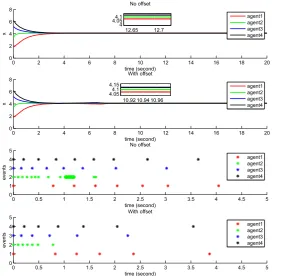
3.5 Input quantization case with logarithmic quantizer . . . 38

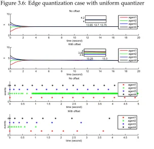
3.6 Edge quantization case with uniform quantizer . . . 39

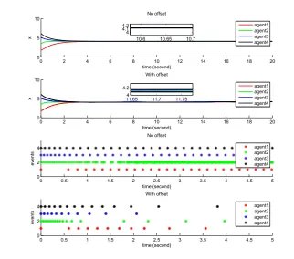
3.7 Edge quantization case with logarithmic quantizer . . . 39

4.1 Graph topology . . . 50

4.2 Comparison of state trajectories . . . 51

4.3 State trajectories for all agents and edge event times for agents 1 and 2 triggered over edge e1 . . . 52

5.1 Graph topology used in simulations . . . 68

5.2 Top: the evolutions of the generalized coordinate and velocity of agent 1. Bottom: the trigger event times of agent 1 . . . 69

5.3 Performance of controller (5.9) using SDTF (5.26). We set βi = 2.4. From top to bottom: 1) the rendezvous of the generalized coordinates; 2) the evolution of βikvi(t)k; 3) event times for each agent. . . 69 5.4 Performance of controller (5.9) using TDTF (5.27). We setκiexp(−εit) =

0.1 exp(−0.2t). From top to bottom: 1) the rendezvous of the gener-alized coordinates; 2) the evolution of κiexp(−εit); 3) event times for each agent. . . 70 5.5 Performance of controller (5.9) with MTF (5.28). We set βi = 2.4

and κiexp(−εit) = 0.1 exp(−0.2t). From top to bottom: 1) the ren-dezvous of the generalized coordinates; 2) the evolution ofβ_ikv_i(t)k+ κiexp(−εit); 3) event times for each agent. . . 70 5.6 Diagram for proof of Theorem 8. The red region is S(t), in which

˙

V(t) < 0 for allt ≥ 0. The blue region is T(t), in which ˙V(t) is sign indefinite. A trajectory of (5.36) is shown with the black curve. At

t = T1, it is shown in Part 2 that the trajectory of (5.36) is such that

ku(T1)k< X,kv(T1)k<Y and thus the trajectory does not leaveS(t).

The sign indefiniteness of ˙V(t)inT(t)arises due to the terms linear in kukandkvkin (5.49), i.e. the terms containing ¯ω(t)(coefficientsA5(t)

and A6(µ,t) in (5.50)). Because ¯ω(t) goes to zero at an exponential

rate, so do the coefficients A5(t)and A6(µ,t). Examining the

inequal-ities detailed in Corollary 1 as applied to p(kuk,kvk) in (5.50), it is straightforward to conclude that for a fixed µ₆∗, the exponential decay

of A5,A6implies that the regionT(t)shrinks towards the origin at an

exponential rate. In other words,ϑ(t)andϕ(t)monotonically increase

until ϑ(t) =X andϕ(t) =Y, at which point T(t) = [0, 0]. This

corre-sponds to the dotted red and blue lines, which show, respectively, the time-varying boundaries ofS(t)andT(t). The solid red and blue lines show respectively, the boundaries of S(t) and T (t), which are time-invariant. Exponential convergence to the leader-follower objective is discussed inPart 3making using ofT2. . . 80

5.7 Two-link manipulator, generalized coordinatesq= [q1,q2]> . . . 86 5.8 Simulation results for controller (5.9) under trigger function (5.11).

From top to bottom: the plots the generalized coordinates; the plots of generalised velocities of all the follower manipulators; the plot of variable gainµi(t); the plot of trigger events . . . 87 5.9 Simulation results for controller (5.29) under trigger function (5.31).

From top to bottom: the plots the generalized coordinates; the plots of generalised velocities of all the follower manipulators; the plot of trigger events . . . 88 5.10 Simulation results for controller (5.58) under trigger function (5.61).

6.1 Examples on rigid and non-rigid formations. (a) non-rigid formation (a deformed formation with dashed lines is shown); (b) minimally rigid formation; (c) rigid but non-minimally rigid formation. . . 94 6.2 Simulation on stabilization control of a double tetrahedron formation

in 3-D space with centralized algorithm. The initial and final positions are denoted by circles and squares, respectively. The initial formation is denoted by dashed lines, and the final formation is denoted by red solid lines. The black star denotes the formation centroid, which is stationary. . . 108 6.3 Exponential convergence of the distance errors with centralized

algo-rithm. . . 109 6.4 Performance of the centralized algorithm. Top: evolution of kδkand

kδkmax=γkR(t)Te(t)k. Bottom: event triggering instants . . . 109

6.5 Simulation on stabilization control of a double tetrahedron formation in 3-D space with distributed algorithm. The initial and final positions are denoted by circles and squares, respectively. The initial formation is denoted by dashed lines, and the final formation is denoted by red solid lines. The black star denotes the formation centroid, which isnot

stationary. . . 110 6.6 Controller performance of the distributed event-triggered formation

system (6.30) with distributed trigger function (6.34). Left: Event in-stants for each agent. Right: Exponential convergence of the distance errors with distributed event controller. . . 111 6.7 Controller performance of the distributed event-based formation

Introduction

1

.

1

Research background

Multi-agent systems (MASs) in general refer to a large-scale system consisting of multiple autonomous agents, which coordinate their actions to achieve a group ob-jective. The word "agent" can refer to autonomous robots, unmanned aerial vehicles (UAVs), or mobile sensors, depending on different control context. The control algo-rithms designed for MASs are usually required to be implemented in a distributed manner, since it is undesirable to collect and process the global information, compute and allocate the control tasks, within a centralized processor. Over the past decade, the development and investigation of MASs has become extremely popular in var-ious research communities (e.g. control, power systems, computer science, social science) due to their great capacity for a broad applications [Ren and Beard, 2008; Nagata and Sasaki, 2002; Ferber, 1999; Pan et al., 2007].

In control community, there are two fundamental tasks in the study of MASs:

• Consensus, where the aim is to reach an agreement regarding certain quan-tities of interest that depend on the states of all agents via local interaction rules. Successful applications of consensus algorithms are found in spacecraft attitude alignment [VanDyke and Hall, 2006; Ren and Beard, 2004], in smart grids [Zhang and Chow, 2012; Rahbari-Asr et al., 2014] and in wireless sensor networks (see [Oliva et al., 2013; Qin et al., 2017a] for a clustering problem) and [Carli and Zampieri, 2010; Seyboth and Allgower, 2013] for a clock synchro-nization problem). Some excellent surveys of recent progress on the research of multi-agent consensus can be found in [Cao et al., 2013; Knorn et al., 2016].

• Formation control aims to design distributed control algorithms such that a group of agents can achieve some pre-defined formations defined by geometric relationships between the agents. The distributed formation control strategies are usually classified into two types: displacement-based approach [Ren, 2007; Dong and Hu, 2016], in which the desired formation is specified by a set of inter-agent relative positions, and distance-based approach [Anderson et al., 2008; Sun et al., 2015b; Oh and Ahn, 2014]1, in which the desired formation is

1_{In this thesis, we use ’rigid formation control’ to represent formation control using a distance-based}

approach.

specified by a set of inter-agent distances. The two approaches have their own distinct properties. We refer the readers to an excellent survey paper [Oh et al., 2015] for detailed discussions on formation control.

In practical applications, agents in MASs are usually resource limited. The re-source here mainly refers to the agents’ on-board devices, such as microprocessors (for processing information and generating control signals), wireless communication devices (for exchanging information among agents), sensors (for measuring relative information between neighbouring agents) and actuators (for driving the agents). The resource limitations partly arise from the fact that these on-board devices are composed of digital components whose performance are restricted by the frequency of the clock references. Thus the procedures of information collection, exchange and processing as well as the generations of control signals can only be implemented in a discrete-time manner even though the agents’ self dynamics are continuous. Ac-cording to the above observations, it is necessary to design distributed algorithms with discrete updating time instants for MASs. The classical approach is to use time-scheduled control scheme (or sampled control scheme) [Isermann, 2013]. When using time-scheduled control scheme, the control updates are determined by a con-stant sampling period, and between updates the control signals are held concon-stant via zero-order hold techniques. Some recent effort regarding the application of time-scheduled control in MASs can refer to [Xie et al., 2009; Liu et al., 2010; Yu et al., 2011; Gao and Wang, 2011; Xiao and Chen, 2012]. However, using time-scheduled control may be conservative in terms of the number of control updates, since the constant sampling period has to guarantee stability in the worst-case scenario [Sey-both, 2010]. Under this background, the event-scheduled control scheme [Tabuada, 2007; Heemels et al., 2008; Lehmann and Lunze, 2009; Donkers and Heemels, 2012; Wang and Lemmon, 2011] have been introduced into the field of MASs. While both schemes update at discrete time instants, in comparison with the time-scheduled scheme, the event-scheduled scheme has a distinctive advantage when applied in MASs as it can generate updating events aperiodically and adaptively, which has the potential to reduce as much the requirement of processing and actuating resources as possible. Some brief introduction for the recent progress regarding event-triggered control in MASs can be found in [Qin et al., 2016]. InChapter2, we will also provide a detailed review on the basic event-triggered schemes for MASs, appeared in recent literature. We note that there also have been some work that reports successful appli-cations of event-triggered strategies in different coordination tasks [Guinaldo et al., 2013; Araújo et al., 2014; Wang et al., 2017a].

consensus tasks (results are presented in Chapters 3-5). We then solve a distance-based formation control problem, by using event-triggered control algorithms. Note that the distance-based formation control problem was proposed under a practical constraint that agents cannot share a knowledge of a global coordinate system. Our proposed event-triggered algorithms can deal with this practical constraint, as well.

1

.

2

Contributions and Outline

In this section, we present the outline and summarize the main contributions, of the thesis. We remark that at the beginning of each main chapter, a more detailed lit-erature review with comparison to existing work will be provided for each research topic.

Chapter 1presents a general introduction to the research background and some mo-tivations for the research topics to be discussed in this thesis.

Chapter 2 provides mathematical notations and theoretical preliminaries on graph theory (which focuses on undirected graphs). A general revisit to the event-triggered consensus problem with the review of relevant literature is also provided in this chapter.

Chapter 3 develops two event-triggered control algorithms with quantized relative state measurementsto achieve consensus for a multi-agent system where each agent is modelled by single integrator dynamics and the network topology is captured by an undirected graph. Both uniform and logarithmic quantizers are considered.

The main contributions of this chapter are summarised as follows:

• We propose event-triggered control algorithms in which the updates of the control inputs and calculations of the trigger conditions are both implemented with onlyquantized relative information.

• We establish the fact that the offsets added to the trigger conditions are neces-sary to eliminate Zeno behaviour for each agent when designing distributed, event-triggered consensus algorithms with quantized information and presents detailed discussions on how to design constant offsets with a priori knowledge of the graph topology and quantization gain.

unsynchronized clock case, are studied. In the synchronized clock case, all agents are activated simultaneously to measure the relative state information over edge links under a global clock. Edge events are defined and their occurrences trigger the up-date of control inputs for the two agents sharing a link. We show that average con-sensus can be achieved with our proposed algorithm. In the unsynchronized clock case, each agent executes its control algorithm under its own clock which is not synchronized with other agents’ clocks. An edge event only triggers control input update for an individual agent. We show that all agents will reach consensus in a totally asynchronous manner.

The main contributions of this chapter are two-fold:

• The synchronized clock case provides new insights to the edge-event-triggered consensus problem with much simpler trigger conditions. Moreover, when em-ploying our algorithm, agents only need to use relative information measured in its own local coordinate frame.

• The unsynchronized clock case provides a generalised framework for edge-event-triggered algorithms where agents can be activated to execute the con-sensus task at different starting times. The case involving synchronized clocks thus can be regarded as a special case.

Chapter 5 proposes three different distributed event-triggered control algorithms to achieve leader-follower consensus for a network of Euler-Lagrange agents. We first propose two model-independent algorithms for a subclass of Euler-Lagrange agents whose dynamics do not have the vector of gravitational potential forces. A variable-gain algorithm is employed when the sensing graph is undirected. When the sensing graph is directed, a constant-gain algorithm is employed. When the Euler-Lagrange agents have dynamics which include the vector of gravitational potential forces, an adaptive algorithm is proposed.

Our main contributions in this chapter are the following:

• A globally asymptotically stable variable-gain model-independent algorithm is proposed for agents on undirected graphs. The variable-gain controller allows for fully distributed and arbitrary design of parameters in both the control algorithm and trigger function.

• A model-independent, constant-gain algorithm applicable for directed graphs is proposed to achieve leader-follower consensus for networked Euler-Lagrange agents semi-globally, exponentially fast. The control gains are designed to ex-ceed several lower bounding inequalities which require limited knowledge of bounds on the matrices describing the agent dynamics, bounds on network topology information and bounds on the initial conditions.

net-works. The algorithm requires more information about the agent dynamics but allows for uncertain agent parameters.

• All three proposed algorithms use only piecewise constant control inputs, which have the benefit of reducing actuator updates and thus conserving energy re-sources. Furthermore, each agent only updates its control inputs at its own event times, and does not require knowledge of the trigger times of neighbour-ing agents.

Chapter 6 discusses cooperative stabilization control of distance-based formations via an event-triggered approach. We first design a centralized event-triggered forma-tion control system, in which a central event controller determines the next trigger-ing time and broadcasts the event signal to all the agents for control inputs update. We then build on this centralized approach to propose a distributed event control strategy, in which each agent can use its local trigger events and local information to update the control inputs at its own event times. For both cases, the triggering condition, triggering behaviour and system convergence are discussed in detail.

The contributions of this chapter are stated as follows:

• For the first time, we propose and apply event-triggered strategies to distance-based formation control tasks.

• We prove local stability of the formation system for both centralized and dis-tributed event-based controllers, and show that, in fact, convergence is expo-nentially fast. The exponential stability of the formation control system has important implications relating to robustness issues.

Preliminary

2

.

1

Notations

The notations used in this thesis are those standard in systems and control literature. We useNto denote the set of all natural numbers. LetRndenote then-dimensional Euclidean space andRm×n _{denote the set ofm×n real matrices. The transpose of a} vector or matrixM is given byM>. The rank, image and null space of a matrixM are denoted by rank(M), Im(M)and ker(M), respectively.The i-th smallest eigenvalue of a symmetric matrix M is denoted by λi(M). Let x = [x1, . . . ,xn]> where xi ∈

Rn×n _{and n > 1. Then diag{x}denotes a (block) diagonal matrix with the (block)} elements of x on its diagonal, i.e. diag{x₁, ...,xn}. A symmetric matrix A ∈ Rn×n which is positive definite (respectively, non-negative definite) is denoted by A > 0 (respectively, A ≥ 0). For two symmetric matrices A,B, the expression A > B is equivalent to A−B>0. The n×n identity matrix is In and 1n denotes an n-tuple column vector of all ones. The n×1 column vector of all zeros is denoted by 0n. The symbol⊗ denotes the Kronecker product. The Euclidean norm of a vector, and the matrix norm induced by the Euclidean norm, is denoted by k · k. We let kMk_F denote the Frobenius norm for a matrix M. Note that there holds kMk ≤ kMk_F for any matrix M. For the space of piecewise continuous, bounded vector functions, the norm is defined as kfkL_∞ = supkf(t)k < ∞ and the space is denoted by L∞.

The spaceL_p for 1 ≤ p < ∞is defined as the set of all piecewise continuous vector functions such that kfkLp =

R∞

0 kf(t)kpdt 1/p

< ∞ where p refers to the type of

p-norm.

2

.

2

Event-triggered consensus: a revisit

2.2.1 The consensus problem

Consider a MAS consisting of n agents with continuous-time single-integrator dy-namics

˙

xi(t) =ui(t) (2.1)

where xi(t)∈R is the state of agentiandui(t)is the control input. The objective of consensus is to ensure all agents reach a common state value, i.e. x1= x2 =· · ·= xn. It is required that agent i can only take local information (information between agent i and its neighbours) into account to reach consensus. For this purpose, we need to describe the interactions between the agents. A well-known approach is to model the neighbouring relations by a graphG with vertex set V = {v1,v2, . . . ,vn} and edge set E = {e1,e2, . . . ,em} ⊂ V × V 1. The neighbour set Ni of vertex vi is defined as N_i := {vj ∈ V : (vi,vj) ∈ E }. The unweighted adjacency matrix A = A(G) = (aij) is a n×n matrix given by aij = 1, if and only if (vi,vj) ∈ E, and aij = 0, otherwise. If there is an edge (vi,vj) ∈ E, then vertexes vi,vj are said to be adjacent. A path of length r from a vertex vi to a vertex vj is a sequence of r+1 distinct vertices starting with vi and ending with vj such that consecutive vertices are adjacent. If there is a path between any two vertices of the graph G, then G is called connected. Let D be the n×n diagonal matrix of di’s, where the degree di of each vertex i is defined as di = ∑nj=1aij. The Laplacian matrix of G is a symmetric positive semi-definite matrix given by L = D − A. For a connected graph, the Laplacian matrix L has a single zero eigenvalue and the corresponding eigenvector is the vector of ones. All other eigenvalues are positive and real. The eigenvalues of L can be ordered as 0 = λ1(L) < λ2(L) ≤ . . . ≤ λn(L) [Ren and Beard, 2008].

We define an auxiliary variable gi(t)for agenti:

gi(t) =

∑

(xi(t)−xj(t)) (2.2)

The consensus controller is typically designed as follows:

ui(t) =−gi(t) (2.3) or some variation of the above. By using the Laplacian matrix L, the closed loop form of the MAS with agents having dynamics (2.1) and control inputs (2.3) can be written as

˙

x(t) =−g(t) =−Lx(t) (2.4) where g(t) = [g1(t)· · ·gn(t)]>∈Rn andx(t) = [x1(t)· · ·xn(t)]> ∈Rn.

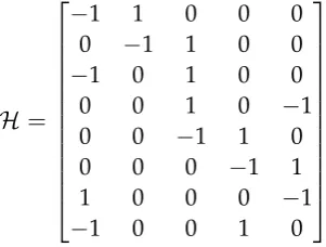
Another important matrix representation of an undirected graph G is the inci-dence matrixH =hri ∈Rm×n(for more information, see [Zelazo and Mesbahi, 2011; Bapat, 2010; Mesbahi and Egerstedt, 2010]. The incidence matrix relates the edges to the vertexes, whose entries are defined as (with arbitrarily chosen edge orientations):

h_ri =    

  

−1, if vertexvi is the terminal vertex of edgeer 1, if vertexv_i is the initial vertex of edgeer 0, otherwise

(2.5)

Note that the Laplacian matrix for an undirected graph can be written asL=H>H. The incidence matrixHcan be divided into two sub matrices: the in-incidence matrix and the out-incidence matrix. Following the definitions in [Zeng et al., 2016], each entry of them×nin-incidence matrixHJ is denoted as

(hJ)

ri = (

−1, if vertexvi is the terminal node ofr-th edge

0, otherwise (2.6)

and each entry of them×nout-incidence matrixHNis denoted as

(hN)

ri = (

1, if vertexvi is the initial node ofr-th edge

0, otherwise (2.7)

It is obvious that H=HJ+HN.

By using the incidence matrix H, we can construct the relative state vector as an image of Hfrom the state vectorx:

z(t) =Hx(t) (2.8) where z(t) = [z1(t)· · ·zm(t)]> ∈ Rm with zr ∈ R being the relative state for the vertex pair defined by ther-th edgeer. Then, the consensus dynamics (2.4) can also be reformulated as:

˙

x(t) =−H>z(t) (2.9) We use Example 1 to show how to construct the Laplacian matrix, incidence matrix, in-incidence matrix and out-incidence matrix for a given undirected graph.

For an undirected graph Gand its corresponding Laplacian matrix and incidence matrix, we have the following lemmas.

Lemma 1 ([Dimarogonas and Johansson, 2010]). If G is undirected and connected, the matrixHH> and the Laplacian matrixLboth have non-negative eigenvalues and moreover the same positive ones.

Lemma 2([Guo and Dimarogonas, 2013]). IfGis undirected and connected, thenz>HH>z≥

λ2(L)kzk2.

and broadcast the self-state (xi(t)) to its neighbours. This approach requires agents to be

aligned with a common coordinate system. Another approach is to let each agent sense the relative states (xj(t)−xi(t)) between its neighbours and itself by using sensors, for example,

stereo cameras. In this approach, only local coordinate systems are required. To equip both wireless communication devices and relative state sensors on agents for consensus tasks can be regarded as a waste of resources on hardware cost and energy/process resource consumption, since we usually assume low cost and limited on-board resources for one agent when studying a distributed multi-robot system.

Example 1. An example of the Laplacian matrix and the incidence matrix:

1

2 3 4

5 6

1

2 3 4

5 6

Figure 2.1: Left: An undirected graph. Right: A corresponding directed graph with arbitrarily chosen edge orientations for constructing the incidence matrix.

The Laplacian matrix of the undirected graph inFig. 2.1 can be written as

L=         

2 −1 0 0 0 −1 −1 2 0 −1 0 0

0 0 2 0 −1 −1 0 −1 0 2 −1 0 0 0 −1 −1 3 −1 −1 0 −1 0 −1 3

         By defining z=           

x1−x2 x2−x4 x3−x5 x3−x6 x4−x5 x5−x6 x1−x6           

we can construct an incidence matrix as follows:

H =           

where the in-incidence matrix and out-incidence matrix can be separately constructed as

HJ =

          

0 −1 0 0 0 0 0 0 0 −1 0 0 0 0 0 0 −1 0 0 0 0 0 0 −1 0 0 0 0 −1 0 0 0 0 0 0 −1 0 0 0 0 0 −1           

HN=

          

1 0 0 0 0 0 0 1 0 0 0 0 0 0 1 0 0 0 0 0 1 0 0 0 0 0 0 1 0 0 0 0 0 0 1 0 1 0 0 0 0 0           

It can be verified thatL=H>H andH =HJ+HN.

2.2.2 Basic trigger schemes

Event-triggered consensus algorithms are usually designed based on the fundamen-tal continuous-time controller (2.3), for which there are two main steps:

• Design a control input which only uses the agents’ state values (xi orzi) at some discrete-time instants.

• Define a state mismatch between the continuous states and the discrete-time state values, then design trigger conditions to determine the time instants for updating the control input.

How to define the state mismatch variable (it is called measurement error in some pa-pers) plays a very important role in the design of event-triggered algorithms, accord-ing to which we can classify widely-adopted event-triggered consensus algorithms in the vast number of literature regarding event-triggered consensus into three types, namely self-measurement-based, edge-measurement-based and local-measurement-based schemes.

2.2.2.1 Self-measurement-based scheme

The self-measurement-based scheme is the first trigger scheme reported in the liter-ature (see [Dimarogonas and Johansson, 2009a,b; Dimarogonas et al., 2012] for some early work) and has been widely developed in the studies of event-triggered consen-sus problem investigating different agent dynamics [Mu et al., 2015; Yang et al., 2016; Garcia et al., 2014; Liu et al., 2016d], and information constraints (e.g. graph topol-ogy, information quantization, communication delays) [Seyboth et al., 2013; Garcia et al., 2013; Yi et al., 2016; Mu et al., 2015; Zhang et al., 2015].

In this scheme, each agent is required to monitor its own state (xi(t)) continuously in a global coordinate system. The interactions among the agents rely on on-board wireless communication devices. Let the event time instants for agent ibe denoted asti₀=0,· · · ,ti_ki,· · ·. The state mismatch for agentiis defined as

Every time an event is triggered,ei(t)is reset to be equal to zero. The control input is described by

ui(t) =−

∑

xi(ti_ki)−xj(tj_kj)

(2.11)

where kj _{= arg min}

l∈N : t ≥ tjl. Fort ∈ [tiki,ti_ki₊₁), t j

kj is the last event time of agent

j. Each agent takes into account the last update value of each of its neighbours in its control law (seeExample2). The control input for agentiis updated both at its own event times ti

0,ti1, . . ., as well as at the event times of its neighbourst

j

0,t

j

1, . . ., j∈ Ni. The closed loop form of the MAS with agent dynamics (2.1) and control input (2.11) can be written as

˙

x(t) =−L 

   

x1(t1_k1)

x2(t2_k2)

.. .

xn(tn_kn) 

   

Note that xi(ti_ki) = xi(t) +ei(t). By substituting this to the above closed-loop form, we obtain

˙

x(t) =−Lx(t)− Le(t) (2.12) This closed loop form is of great importance for the design of trigger conditions and represents the main difference of the self-measurement-based scheme from the other two triggering schemes. We now show how to design a basic, distributed trigger function by using Lyapunov analysis and the closed loop form (2.12).

Consider the following Lyapunov function

V(t) = 1 2x(t)

>_{Lx(t) (2.13)} Its time derivative along the solution of (2.12) is

˙

V(t) =x(t)>Lx˙(t)

=−x(t)>LLx(t)−x(t)>LLe(t)

SinceLis symmetric, we obtaing(t)>= x(t)>L. Then we can upper bound ˙V(t)as ˙

V(t)≤ −kg(t)k2+kLkkg(t)kke(t)k

To guarantee ˙V(t) < 0 ( ˙V(t) < 0 means limt→∞Lx(t) = 0, which implies

consen-sus), we must ensure that ke(t)k ≤ kg(t)k/kLk. For this purpose, we can design a distributed trigger function as follows:

whereβi >0. The trigger condition can be simply formulated as follows: an event for agentiis triggered as soon as the trigger function fi(t) =0 is satisfied. Note thatei(t) is reset at each event time, the trigger condition thus ensureskei(t)k ≤βikgi(t)k. By using a properly selected βi, the trigger condition can ensureke(t)k ≤ kg(t)k/kLk holds for allt ≥0, meaning consensus can be achieved.

Remark 2. The above design procedures follow the ideas proposed in [Dimarogonas and Jo-hansson, 2009a,b; Dimarogonas et al., 2012]. The trigger function(2.14)involves two terms, the error term ei and the comparison term gi, where gi can be calculated by using continuous

communication or measured by relative state sensors (e.g. cameras). To avoid continuous communication, [Dimarogonas and Johansson, 2009a,b; Dimarogonas et al., 2012] assumes each agent monitors the relative states using additional sensors. However, this assumption increases the cost for constructing the system since both wireless communication devices and relative state sensors are equipped. We note that the requirement of continuous relative measurement has been removed in [Garcia et al., 2013; Seyboth et al., 2013], by replacing the comparison term (gi) with state values measured at discrete-time instants and time-dependent

functions, respectively. The two ideas were then widely adopted in the follow-up work (e.g. [Yang et al., 2016; Liu et al., 2016d]) using agent-measurement-based scheme. According to this, we choose to say that, when using the self-measurement-based scheme, each agent only needs to monitor its self state continuously rather than measuring relative states continu-ously.

Now we record two features of the self-measurement-based scheme and present both its advantages and disadvantages.

• Each agent uses discrete-time state values at both its own and its neighbours’ event time instants to update the control input. For this purpose, each agent is assumed to be equipped with wireless communication devices to broadcast the discrete-time state values to its neighbours.

• Each agent monitors its own state continuously to calculate the state mismatch (2.10) and determine event time instants. The state measurement for each agent has to be with respect to a global coordinate system. For example, UAVs use Global Positioning System (GPS) to measure their own position information. Advantages: Each agent only needs to broadcast its discrete-time state values at specific time instants, and therefore continuous communications among the agents are avoided. On-board communication resources can be saved significantly.

2.2.2.2 Edge-measurement-based scheme

The edge-measurement-based scheme is firstly proposed in [Xiao et al., 2012, 2015] and has been further developed by numerous papers, e.g. [Cao et al., 2015; Wei et al., 2016; Cao et al., 2016; Wei et al., 2017; Xu et al., 2017].

In the edge-measurement-based scheme, it is assumed that for each edgeer con-necting agentsi and j, both agents iand j measure the relative statezr over er con-tinuously. The sequence of event-triggered executions for edge er (meaning agents

i,jlinked by er) is denoted by t0r = 0,tr1r,· · · ,t r

kr,· · ·. At trkr, the two linked agents update their control inputs simultaneously. For time t ∈[tr_kr,tr_kr+1), the relative state mismatch over edgeer is defined as

er(t) =zr(trkr)−zr(t), r =1, . . . ,m (2.15) We note that er(t) is actually calculated by agents i and j linked by er separately using their own on-board processors. For agenti, which is one of the agent pair(i,j) linked byer, the control input is designed as follows:

ui(t) =

∑

xj(trkr)−xi(trkr)

(2.16)

for t ∈ [tr_kr,tr_kr+1). Note that only partial information xj(trkr)−xi(trkr) in the control input is updated attr_kr (seeExample2).

According to (2.9), we can construct the closed loop form of agent (2.1) with control input (2.16) as

˙

x(t) =−H> 

    

z1(t1_k1) z2(t2_k2)

.. .

zm(tm_km) 

    

(2.17)

Substituting the state mismatch (2.15) into (2.17) leads to ˙

x(t) =−H>z(t)− H>e(t) (2.18) wherez(t) = [z1(t),z2(t), . . . ,zm(t)]> ∈Rmande(t) = [e1(t),e2(t), . . . ,em(t)]>∈Rm. We now show how to use this closed loop form and the Lyapunov function (2.13) to design a basic edge trigger function.

The time derivative of (2.13) along the solution of (2.18) yields ˙

V(t) =x(t)>Lx˙(t)

SinceG is undirected and connected, by applyingLemma2, we have ˙

V(t)≤ −λ2(L)kz(t)k2+kz(t)kkHH>ke(t)k

We then design an edge trigger function as follows:

fr(t) =ker(t)k −βrkzr(t)k (2.19) with βr > 0. The selection of βr must guarantee ˙V(t)< 0, which means consensus can be achieved.

We also record two features of the edge-measurement-based scheme and summa-rize both its advantages and disadvantages.

• The trigger events are defined over edges rather than agents. An agent may have multiple edge trigger conditions, whose number is determined by the amount of its edges links. Every time an edge trigger condition is satisfied, two agents linked by this edge must update their control inputs simultaneously.

• Each agent measures the relative states over its connected edges to determine edge events. The measurement is executed in each agent’s own local coordinate system.

Advantages: The algorithms based on the edge-event-based scheme can be im-plemented in a totally coordinate-free manner, which extends the application circum-stances.

Disadvantages: The control input (2.16) of agentihas to be updated at the event times of all edges it links. This may also result in a very frequent control input updates. Furthermore, measuring relative states is more complicated and unreliable when compared to measuring self states in practical applications.

2.2.2.3 Local-measurement-based scheme

The local-measurement-based scheme was first proposed in [Fan et al., 2013]. After that, the trigger scheme was widely used and developed by researchers, e.g. in [Liu et al., 2016b,c,a; Hu et al., 2016, 2017; Fan et al., 2015; Li et al., 2015; Zhu et al., 2014; Zhu and Jiang, 2015].

In the local-measurement-based scheme, we let gi(t)(defined in (2.2)) represent the real-time average state of agent iand its neighbours in agent i’s local coordinate system. Agent i monitors gi(t) continuously. The sequence of event-triggered exe-cutions for agent iis ti₀ = 0,ti₁, . . . ,ti_ki, . . .. The state mismatch for agenti is defined as

The control input is designed as follows:

ui(t) =−gi(ti_ki)

=

∑

xj(ti_ki)−xi(ti_ki)

(2.21)

fort ∈[ti_ki,ti_ki₊₁). The control input is only updated at agenti’s own event times. The closed loop form of agent dynamics (2.1) with control input (2.21) is formulated as follows:

˙

x(t) =− 

   

g1(t1_k1)

g2(t2_k2)

.. .

gn(tn_kn) 

   

(2.22)

By substituting (2.20) into (2.22), we obtain ˙

x(t) =−g(t)−e(t) (2.23) wheree(t) = [e1(t),e2(t), . . . ,en(t)]> ∈Rn. We now design a trigger function accord-ing to the Lyapunov function (2.13) and the dynamics (2.23). The derivative of (2.13) along the solution of (2.23) is

˙

V(t) =−g(t)>g(t)−g(t)e(t) (2.24) Then the upper bound of ˙V(t)can be simply calculated as

˙

V(t)≤ −kg(t)k2_{+kg(t)kke(t)k (2.25)}

It is then straightforward to design the trigger function as

fi(t) =kei(t)k −βikgi(t)k (2.26) where βi ∈ (0, 1). Every time fi(t) = 0 is satisfied, ei(t)is reset and thus ˙V(t) < 0 can be guaranteed.

As before, we record the features of the local-measurement-based scheme and summarise both its advantages and disadvantages.

• Each agent has its own isolated trigger conditions. The updates of each agent’s control input are only determined by its own trigger conditions.

• The state mismatch is defined according to each agent’s measurements of rela-tive states in its own local coordinate system.

control input at its own event times; thus the control input updating times can be significantly reduced.

Disadvantages: Similarly, to obtain accurate relative state measurements is com-plicated in practical applications.

We now present an example to intuitively display the differences of the control input updates in the three trigger schemes.

Example 2. Now we present three examples to illustrate the control input updates for the three trigger schemes.

1

2

3

4

5

6

Figure 2.2: Communication topology for the illustration of the self-measurement-based scheme.

Firstly, we describe the updates of agent2’s control input inFig.2.2 to illustrate the self-measurement-based scheme. At time t0,t0 = 0, the control input of agent2 can be written as

u2(t) =x1(t0)−x2(t0) +x3(t0)−x2(t0)

Assuming that the starting trigger times (t1

1, t21, t31) for agents1, 2, 3satisfy t11 <t21 < t31 <

min{t1₂,t2₂,t3₂}. At t1₁, agent2 receives the state update x1(t11)from agent 1, and then the control input changes to

u2(t) =x1(t11)−x2(t0) +x3(t0)−x2(t0)

At t2₁, agent2updates its own state, then

u2(t) =x1(t11)−x2(t21)+x3(t0)−x2(t21)

At t3₁, agent2receives the state update x3(t3₁)from agent3and changes the control input as u2(t) =x1(t11)−x2(t21) +x3(t31)−x2(t21)

Secondly, we turn to the edge-measurement-based scheme. As shown inFig. 2.3. Agent

2 measures the relative states x1−x2 over e1 (linking agents 1 and 2) and x2−x4 over e2 (linking agents 2 and 4) in its own local coordinate system. At time t0, the control input is

u2(t) =x1(t0)−x2(t0) +x3(t0)−x2(t0)

1

2

3

4

5

6

Figure 2.3: Sensing topology for the illustration of both the edge-measurement-based scheme and the local-measurement-based scheme.

min{t1

2,t22}. At t11, the control input changes to

u2(t) =x1(t11)−x2(t11)+x3(t0)−x2(t0)

Then at t2₁, the control input is

u2(t) =x1(t11)−x2(t11) +x3(t21)−x2(t21)

Lastly, we move to illustrate the local-measurement-based scheme. Agent 2 measures x1−x2and x2−x4in its own local coordinate system. At t0, the control input for agent 2 is:

u2(t) =x1(t0)−x2(t0) +x3(t0)−x2(t0)

At t2

1, which is the first trigger time of agent2, the control input is updated as u2(t) =x1(t21)−x2(t21) +x3(t21)−x2(t21)

At the second trigger time t2₂, the control input changes to

u2(t) =x1(t22)−x2(t22) +x3(t22)−x2(t22)

2.2.3 Zeno behaviour

Zeno behaviour is a key issue when designing event-scheduled control systems. We first provide a formal definition of Zeno behaviour:

Definition 1. Let a finite time interval be tZ = [a,b]where0 ≤ a < b< ∞. If, for some

finite k≥0, there is a sequence of event triggers{ti_k, ...,ti_∞} ∈[a,b]then the system exhibits Zeno behaviour.

definitions of this concept of Zeno behaviour are not provided in [Seyboth, 2010; Qin et al., 2017b] or in other literature, we call this concept of Zeno behaviour asConcept 2, noting it is different fromDefinition1, for later reference.

An example presented in [Qin et al., 2017b] can be used to illustrate the differ-ences betweenDefinition1 andConcept2: if the inter-event timeti_k+1−ti_kis bounded below by 1_t, where t denotes a continuous time, then the lower bound 1_t tends to 0 when t → ∞. There might be accumulation events as t → ∞. In Concept 2, this accumulation of trigger events at t → ∞ is also called Zeno behaviour. However, in Definition1, this is not Zeno behaviour as the definition is only valid in at finite time.

Remark 3. In this thesis, we adoptDefinition1 as the formal definition of Zeno behaviour. however, it is also obvious that, if we can exclude Zeno behaviour according to Concept 2, then Zeno behaviour defined inDefinition1 does not exist, either.

In the sequel, we will follow the idea presented in [Sun et al., 2016a] to show that how Zeno behaviour may happen when using the basic event-triggered consensus schemes introduced above.

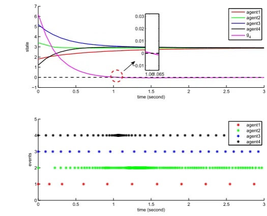
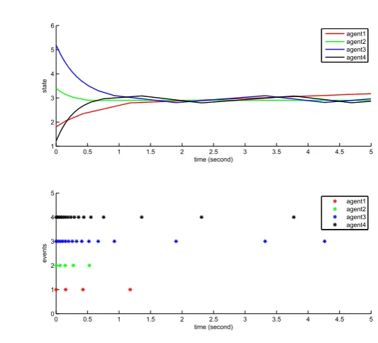
We first use a simulation to show the trigger performance of agents with dynam-ics (2.1) and with control inputs (2.21) and trigger functions (2.26).

0 0.5 1 1.5 2 2.5 3

−1 0 1 2 3 4 5 6 7

time (second)

state

agent1 agent2 agent3 agent4 g₄

0 0.5 1 1.5 2 2.5 3

0 1 2 3 4 5

time (second)

events

agent1 agent2 agent3 agent4 1.061.065

−0.01 0 0.01 0.02 0.03

Figure 2.4: State trajectories and trigger performance of agents with dynamics (2.1) and with control input (2.21) and trigger function (2.26).

From Fig. 2.4, it is observed that agent 4 shows a dense trigger phenomenon when the comparison term g4 crosses zero at some finite time 2. Referring to the

2_{We emphasis that g}

i is thei-th element of vectorg, which may cross zero several times at some

numerical data in the simulation shows that the minimum inter-event time is 0.00005 seconds, which is equal to the fixed time step of our settings in MATLAB. From the viewpoint of the experiment, this dense trigger phenomenon can be seen as Zeno behaviour. We note that the issue of Zeno behaviour at zero-crossing points of the state-dependent comparison threshold has been theoretically proved in [Sun et al., 2017]. We refer interested readers to this comment paper.

For three basic trigger schemes, all of the comparison terms might behave zero-crossing phenomenon, which means Zeno behaviour cannot be completed excluded by each agent when using the basic trigger schemes. Now we show three Zeno-free approaches proposed in the literature.

2.2.4 Zeno-free approaches

In the last subsection we have concluded that Zeno behaviour occurs when ti k+1− ti_k →0 at some finite time instants and the reason is that the comparison thresholds in the trigger functions cross zero. Thus there are two intuitive idea to exclude Zeno behaviour. One is to modify the comparison thresholds for which zero-crossing phe-nomenon does not appear. By following this idea, we will introduce two modified trigger functions with either a time-dependent comparison threshold or a static com-parison threshold. Another idea is to directly add a strictly positive inter-event time interval. We will talk about this at the end of this subsection.

2.2.4.1 Time-dependent trigger function

The intuitive idea of the time-dependent trigger function is to replace the state-dependent comparison term in the trigger functions, e.g. (2.14), (2.19), (2.26), by a non-negative, time-dependent continuous function hi(t), which can be formulated as

fi(t) =kei(t)k −hi(t) (2.27) In [Sun et al., 2016a], a general type ofhi(t)is designed and analysed, which satisfies

hi(t)∈ L∞,hi(t)>0 for all finite timetandhi(∞) =0. Sincehi(t)is strictly positive at any finite time, it takes time for kei(t)k to increase from zero at tik to be equal to hi(t) so that Zeno behaviour is excluded. By finding an upper bound bi of the evolution speed _dtdkei(t)k, a lower bound for the inter-event time ti_k+1−ti_k can be simply calculated as h_i(ti

k+1)/bi, which is strictly positive for any finite time tik+1,

and thus Zeno behaviour is excluded.

0 0.5 1 1.5 2 2.5 3 3.5 4 4.5 5 1

2 3 4 5 6

time (second)

state

agent1 agent2 agent3 agent4

0 0.5 1 1.5 2 2.5 3 3.5 4 4.5 5 0

1 2 3 4 5

time (second)

events

agent1 agent2 agent3 agent4

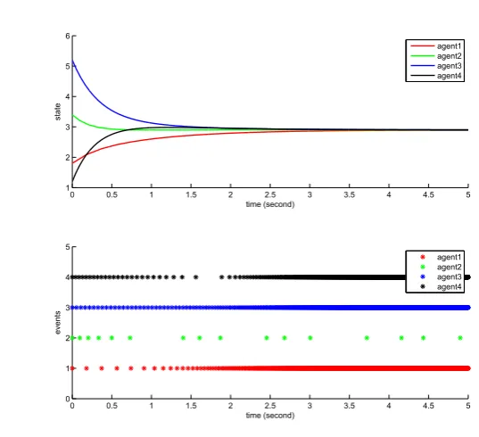
Figure 2.5: State trajectories and trigger performance of agents (2.1) with control input (2.21) and time-dependent trigger function (2.28). We setαi =3 for all agents .

We conclude that the trigger behaviour inFig. 2.5 is Zeno-free in terms ofDefinition 1, but is not Zeno-free in terms of Concept 2. It is still possible to use a time-dependent trigger function to exclude Zeno behaviour as presented inConcept2 by carefully designing the decay rate of hi(t). This idea is first proposed in [Seyboth, 2010; Seyboth et al., 2013], wherehi(t)is chosen as

hi(t) =ciexp−αit (2.28) with ci,αi > 0. The exponential decay rate αi is required to be less than a specific upper bound, which is calculated according to the system evolution rate (e.g. related to the network connectivityλ2). By using carefully designed, time-dependent trigger

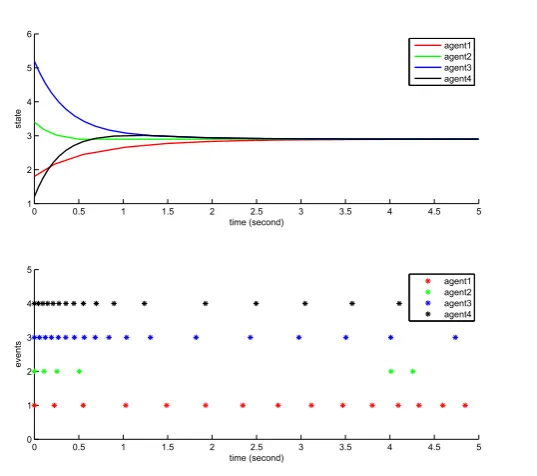
function, a strictly positive, constant lower bound of the inter-event timeti_k+1−ti_kcan be obtained, which excludes the possibility of accumulation events when t ∈ [0,∞) (seeFig. 2.6 for the trigger performance whenα_i is selected small enough).

Though using a pre-designed time-dependent trigger function shows nice trigger performance, there exist two constraints:

• The studied system has to be exponential stable.

• The design of the decay rate requires global informations.

0 0.5 1 1.5 2 2.5 3 3.5 4 4.5 5 1

2 3 4 5 6

time (second)

state

agent1 agent2 agent3 agent4

0 0.5 1 1.5 2 2.5 3 3.5 4 4.5 5 0

1 2 3 4 5

time (second)

events

agent1 agent2 agent3 agent4

Figure 2.6: State trajectories and trigger performance of agents (2.1) with control inputs (2.21) and time-dependent trigger functions (2.28). The parameterαi is set as

1.5 for all agents .

2.2.4.2 Static trigger function

The idea of using a static trigger function to exclude Zeno behaviour can be found in [Zhu et al., 2014; Mu et al., 2014; Seyboth, 2010].

A static trigger function is usually designed as

0 0.5 1 1.5 2 2.5 3 3.5 4 4.5 5 1

2 3 4 5 6

time (second)

state

agent1 agent2 agent3 agent4

0 0.5 1 1.5 2 2.5 3 3.5 4 4.5 5 0

1 2 3 4 5

time (second)

events

agent1 agent2 agent3 agent4

Figure 2.7: State trajectories and trigger performance of agents (2.1) with control input (2.21) and static trigger function (2.29). ci is chosen to be 0.5 for all agents.

2.2.4.3 Time-regulation trigger condition

The time regulation idea is originally proposed in [Nowzari and Cortés, 2014; Fan et al., 2015] and is gaining attention.

We use the equations in [Fan et al., 2015] to illustrate the idea of using time-regulation trigger condition. The next event timetki+1 for agentiis determined by

tki+1= tki +max{τki,ci} (2.30) whereci is a strictly positive andτki is determined by

τkr = inf

t>tkr

{t−tkr|fi(t) =0} (2.31)

where fi(t)is the trigger function (2.26).

By observing the above equations, we see that the time-regulation idea is straight-forward by directly adding a strictly positive, minimum inter-event timeci between two consecutive trigger events, thus Zeno behaviour (Concept 2) can be well ex-cluded by each agent. To ensure convergence, the minimum inter-event time has to be less than a finite upper bound. Though this is a straightforward idea, how to calculate the upper bound of ci is actually quite challenging, especially when the studied system has complex agent dynamics or network topology.

2

.

3

Chapter summary

Event-Triggered Consensus with

Quantized Relative Information

3

.

1

Introduction

Event-triggered consensus [Dimarogonas et al., 2012; Seyboth et al., 2013; Fan et al., 2013] and quantized consensus [Nedi´c et al., 2009; Liu et al., 2012; Guo, 2011; Cera-gioli et al., 2011] have been widely investigated in recent years. Note that quantized algorithms are considered because they reduce the requirement of measurement, and event-triggered algorithms are designed to reduce the requirement of control updates. However, implementing both of them together to further minimize the pro-cessing and actuating burden is still relatively unexplored. Some existing work in this area can be found in [Yu and Antsaklis, 2012], [Garcia et al., 2013] and [Zhang et al., 2015]. The work in [Yu and Antsaklis, 2012] first uses quantizedabsolutestate measurements to design event-triggered consensus algorithms for undirected net-works with single integrator agent dynamics. The authors prove that the quantized states of agents achieve consensus asymptotically. In [Garcia et al., 2013], the authors consider a uniform quantizer and prove that all agents will converge to a certain ball whose radius is related to the quantization error. However, both [Yu and Antsak-lis, 2012] and [Garcia et al., 2013] do not provide any analysis on the exclusion of Zeno behaviour [Zhang et al., 2001], which is a key issue when designing event-scheduled systems as Zeno behaviour can cause the collapse of the entire system. In addition, the proposed schemes in [Yu and Antsaklis, 2012] and [Garcia et al., 2013] require each agent to update its own control input at both its own and its neighbours’ trigger time and this may increase the updating frequency significantly. Moreover, the information shared among the agents in these work is measured with respect to a global coordinate. However, for multi-robot systems in 2-dimensional or 3-dimensional space, the assumption that all robots align with a global coordinate system is undesirable for implementing consensus controllers in e.g. a GPS-denied environment. The work in [Zhang et al., 2015] is built on [Garcia et al., 2013], in which the authors further investigate the case of logarithmic quantizer and provide analysis which shows Zeno behaviour does not occur. However, it is worth point-ing out that the trigger conditions proposed in this work useidealstate information

instead of quantized state information. This strong assumption makes the exclusion of Zeno behaviour easier but is not reflective of real world applications since agents with digital sensors and processors actually will not have access to the ideal state information.

In this chapter, we present event-triggered algorithms for solving the consensus problem withquantized sum of relative statesandsum of quantized relative states, respec-tively. The agent dynamic is described by single integrator and the sensing graph is undirected. Both uniform and logarithmic quantizers are considered, which, to-gether with two different controllers, yield four cases of study in this chapter. The quantized information is used to update the control input as well as to determine the next trigger event. We show that approximate consensus can be achieved by the pro-posed algorithms and Zeno behaviour can be completely excluded if constant offsets with some computable lower bounds are added to the trigger conditions.

3

.

2

Additional Preliminaries

3.2.1 Quantizer functions

In this chapter, q(·) : R → R represents a generalised quantization function which includes two types of quantization models, namely uniform quantization and loga-rithmic quantization. We follow the definitions of [Guo, 2011] for these quantizers. Definition 2. A uniform quantizer qu:R→Ris defined as:

qu(x) =∆u[

x

∆u

] (3.1)

where[·]denotes the nearest integer operation and[1₂] =1. ∆uis the quantization gain. Definition 3. A logarithmic quantizer ql :R→Ris defined as:

ql(x) =sign(x)·equ(ln(|x|)) (x6=0) (3.2)

where qu is the uniform quantizer with gain ∆u, as defined in (3.1). In particular, ql(0)is

defined to be zero.

3.2.2 Quantizer properties

Letδ(x) =q(x)−xdenote the quantization error function. For the uniform quantizer qu, the following relation holds

|δu(x)|=|qu(x)−x| ≤ ∆u

2 (3.3)

For the logarithmic quantizerql, we haveδl(x) =ql(x)−x. Then |δl(x)| ≤∆l|x|, ∆l =e

∆u

where∆uis the gain of uniform quantizer in (3.1).

0 0.5 1 1.5 2 0

0.5 1 1.5 2 2.5

x qu

(x)

Uniform quantizer (gainδu=0.2)

Figure 3.1: Uniform quantizer function with the gainδu=0.2.

0 0.5 1 1.5 2

0 0.5 1 1.5 2 2.5

x

ql

(x)

Logarithmic quantizer (gain δu=0.2)

Figure 3.2: Logarithmic quantizer function with the gainδu =0.2.

3

.

3

Problem formulation

Assume that each agent is equipped with sensors which allow measurement of rela-tive states (e.g. xi−xj). We further assume that the relative state sensors have their own processors and can collect the relative state information xi−xj continuously. The sensing graph topology for the relative states is captured by a fixed, undirected graph G with associated incidence matrix H and Laplacian matrixL. That is, if for agentiwe haveaij =1, i.e. the sensors on agentican sensexi−xj. The control unit of agent i can only receive quantized information from its sensors and update the control input at its own event time. The sequence of event-triggered executions for agentiisti

0=0,ti1, . . . ,tik, . . ..

Assume agentiis described by single-integrator dynamics ˙

xi(t) =ui(t) (3.5) for all i ∈ 1, . . . ,n. Since the way of quantizing information is determined by the relative state sensors, the control input can either be thequantized sum of relative states

or the sum of quantized relative states. Accordingly, we design two controllers. The control input 1 is designed as

ui(t) =q

∑

(xi(tik)−xj(tik)) !

(3.6)

while the control input 2 is designed as

ui(t) =

∑

qxi(tik)−xj(tik)