Hernando Carlos Luis Sabau Garcia
A thesis submitted for the degree of Doctor of Philosophy
of
The Australian National University
DECLARATION
T he co n ten ts of th is th esis a re m y own w ork , except w here o th erw ise in d icated .
ACKNOWLEDGEMENTS
I am deeply indebted to my Supervisors, Dr. Trevor S. Breusch and Dr. Anthony D. Hall, for their comments, guidance and constructive criticism. Their help was not restricted to academic matters and their doors were always open for advice and discussion.
Dr. Adrian R. Pagan introduced me to the topic of the Thesis and put me in contact with a rich and interesting literature. To him I want to express my most sincere gratitude. The many references to his work in this Thesis show only a very small fraction of my intellectual debt to him.
Many others in the Department of Statistics, Faculty of Economics and Commerce, ANU, contributed to a stimulating environment. In particular, I would like to thank Professor R. Deane Terrell without whose support my doctoral studies would not have been possible, and Dr. John J. Beggs who always offered constructive criticism and was enthusiastic in undertaking joint work with me. My thanks also go to Mrs. Daniele Elliot who typed the manuscript with great skill and care.
I gratefully acknowledge the financial support of an ANU Scholarship during the period of my study, and an educative credit from Banco de Mexico. I also want to express my gratitude for the institutional support of the Centro de Investigaciön y Docencia Economicas, A. C. (CIDE).
To my daughters Lucfa and Ana I thank for putting up with a not always understanding father during this period, and to my Mother I thank especially for the time she spent with us in Canberra.
ABSTRACT
This Thesis is concerned with econometric inference in parametric heteroskedastic models. Each moment of the conditional distribution can be seen as a source of information which provides an estimating equation for the parameter vector. Different issues arise in the different moments concerning the identifiability of parameters, the observability of the dependent variable of the estimating equation, and the positivity restrictions implicit in even order moments. Estimators of the identifiable functions of the parameter vector are obtained from orthogonality conditions in each moment. Under symmetry of the distribution, the sources of information corresponding to the first two conditional moments are independent, at least asymptotically, and the information about common parameters is combined in estimation by constructing a matrix weighted average. Estimation procedures under normality are viewed in a maximum likelihood framework, and generalized method of moments estimation provides the setup for the analysis of more general distributions. The separation of the information into its moment source constitutes a basic element for diagnostic testing of the model. The implications of different forms of misspecification are analyzed and robustness properties are established for some leading cases, especially the ARCH class of models. A general framework is presented for diagnostic testing of
heteroskedastic models, which includes tests of the coherency of the
information contributed by the two moments, a family of 'consistency tests' which concentrates on the assessment of the first two moments, and a family of 'efficiency tests' which concentrates on checking the specification of moments of order three and higher. The consistency and efficiency tests may be
exogeneity, a n d n o rm ality , a re an aly zed in p a rtic u la r. T he e stim atio n an d diagnostic te s tin g fram ew ork is ex ten d ed to th e inclusion of la te n t v ariab les in th e conditional m ean , such as p a ra m e tric ris k m e a su re s a n d v a ry in g
coefficients, an d also to a m u ltiv a ria te settin g . F in ally , th e problem of
TABLE OF CONTENTS
Page
DECLARATION (ii)
ACKNOWLEDGEMENTS (iii)
ABSTRACT (iv)
CHAPTER 1. INTRODUCTION 1
CHAPTER 2. THE BASIC MODEL 11
§ 2.1. Basic model and notation 11
§ 2.2. Assumptions 18
§ 2.3. Some special cases 24
§2.3.1. Simple heteroskedasticity 24
§ 2.3.2. Amemiya model 26
§ 2.3.3. The Poisson and Poisson-type models 27
§ 2.3.4. The ARCH class of models 29
§ 2.4 Objective and design of Monte Carlo experiments 34 CHAPTER 3. ESTIMATION AND LIKELIHOOD FACTORIZATION 39 § 3.1. Extracting information from the conditional mean 40
§ 3.1.1. The parametric approach 42
§ 3.1.2. A note on semi-parametric approaches 44 § 3.2. Extracting information from the conditional variance 47
§ 3.2.1. Two-stage estimators for a 53
§ 3.2.2. Estimating the identifiable functions in the
variance equation 56
§ 3.3. Combining information from the two conditional
moments 59
§ 3.3.1. Combining information from orthogonality
conditions 60
CHAPTER 4. THE ROBUSTNESS OF THE QUASI-MAXIMUM
LIKELIHOOD ESTIMATOR 81
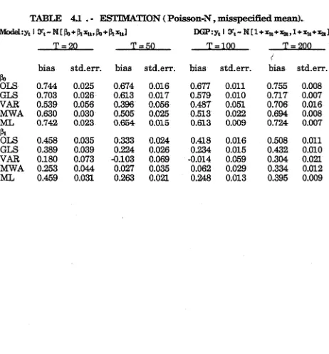
§ 4.1. Some conditions on the likelihood function 82 § 4.2. Specification error in the conditional mean 85 § 4.3. Specification error in the conditional variance 88 § 4.4. Specification error in higher order moments 98 § 4.5. Some com m e n ts on Monte Carlo evidence 96
§ 4.5.1. Specification error in the conditional mean 97 § 4.5.2. Specification error in the conditional variance 100
CHAPTER 5. GENERAL SPECIFICATION TESTS 108
§5.1. Coherency tests 111
§ 5.2. Consistency tests 115
§ 5.2.1. Consistency tests and other tests in the
literature 117
§ 5.2.2. The distribution of consistency test-statistics 122
§ 5.2.3. Some power considerations 129
§ 5.2.4. A simple example 133
§ 5.3. Efficiency tests for higher order moments 134 § 5.4. Comments on some Monte Carlo evidence 139 § 5.4.1. Consistency and coherency tests 139
§ 5.4.2. Efficiency tests 143
CHAPTER 6. TESTING THE MODEL AGAINST SPECIFIC
ALTERNATIVES 152
§ 6.1. The LM test for variable addition 153
§ 6.2. LM tests for autocorrelation and dynamics 156 § 6.2.1. Autocorrelation in the conditional mean 156 § 6.2.2. Dynamics in the conditional mean 158 § 6.2.3. Autocorrelation in the variance equation 160 § 6.2.4. Dynamics in the conditional variance 161
§ 6.3. Parameter stability 163
§6.3.1. Structural break 163
§ 6.3.2. Prediction error tests 165
§ 6.4. LM tests for weak and strong exogeneity 168
§ 6.5. Testing normality 178
§ 6.6. Some comments on the Monte Carlo evidence 183
§ 6.6.1. LM tests for autocorrelation 183
CHAPTER 7. RISK MODELS 189 § 7.1. Param etric risk models and testing for risk effects 190 § 7.2. Estim ation and diagnostic testing of y-risk models 195 §7.2.1. Estim ation of y-risk models 195 § 7.2.2. Consistency and efficiency tests for y-risk
models 200
§ 7.3. Estim ation and diagnostic testing of x-risk models 202 §7.3.1. Estim ation of x-risk models 202 § 7.3.2. Consistency and efficiency tests for x-risk
models 206
CHAPTER 8. VARYING COEFFICIENT HETEROSKEDASTIC
MODELS 215
§ 8.1. Varying coefficients and heteroskedastic models 216 § 8.2. F urther tests for param eter stability and diagnostic
tests for varying coefficient heteroskedastic models 224 § 8.3. Testing for superexogeneity and invariance 227 CHAPTER 9. MULTIVARIATE HETEROSKEDASTIC MODELS 239
§ 9.1. Notation and assumptions 240
§ 9.2. M ultivariate ARCH and some other m ultivariate
heteroskedastic models 243
§ 9.3. Estim ation and likelihood factorization 247
§ 9.4. A note on specification error 254
§ 9.5. Consistency tests 256
§ 9.6. Efficiency tests 260
Appendix to Chapter 9 265
CHAPTER 10. AN EXPLORATION INTO HIGHER ORDER
MOMENTS 272
§ 10.1. Estim ating the first two moments in the presence
of asymmetry 273
§ 10.2. Extracting information from higher order
moments 280
§10.3. Diagnostic testing 294
CHAPTER 11. CONCLUSIONS 298
WITH HETEROSKEDASTIC M ODELS, B y Hernando C. L. Sabau
Page Line
19 21 Says: ... of the variance equation. ...
Should say: ... of th e variance equation. C are should be exercised w hen combining lagged d ep en d en t variables and m ixing conditions (A threya an d P a n tu la [1986]). ... 20 2 Says: . . . 2 on 0, uniform ly in t . F urther, \it a n d ht and
their first two derivatives w ith respect to 0 are bounded from above an d h t is bounded aw ay from zero alm ost everywhere in 0 , uniform ly in t .
Should say: ... 2 on 0 , a nd h t is bounded aw ay from zero alm ost everywhere in © .
20 7 Says: ... Given th is sm oothness ... in th e classical lin e a r model). ...
Should say: ... 20 16 Says: in tro d u c e
Should say: introduce a condition of uniform in teg rab ility (W hite an d Domowitz [1984], page 147):
21 13 Says: . . . o / 0
o-Should say: ... o f 0 o , which is identifiably unique . 21 la s t Says: ... \|/(^)' At \j/(X)
Should say: ... \j/(X)' At \}/(X)
22 18 Says: ... (0.0) - (Cl 7) are sufficient for (A l) - (A9).
remains valid without this continuous differentiability condition.
22 19 Says: ... (Cl2) and (0.3) => (Al) and (A5) ...
Should say: ... (02) and (03) with the continuous differentiability being uniformly in t => (Al) and (A5) ...
22 24 Says: ... in (5) - (7).
Should say: ... in (5) - (7). Now, (C*2) => A l of Andrews [1987] (Andrews in what follows); (C14) - (Cl5) => A5 of Andrews; the mixing conditions in (01) => B1 of Andrews; and (04) - (06) B2 of Andrews. Corollaries 1 and 2 of Andrews then ensure the applicability of his uniform Law of Large Numbers and guarantee the validity of Theorems 3.1 and 3.2 of White and Domowitz without continuity uniformly in t .
49 7 Says: and
Should say: and, provided the expectations exist, 53 8 Says: ... Weiss [1984, 1986a]).
Should say: ... Weiss [1984, 1986a], Davidian and Carroll [1987]). 60 25 Says: which evaluated at some root-T ...
Should say: where for any set of matrices Di ,..., Dm we define the block diagonal matrix
f
Dl 0 . . 0 ^D = diag { D i , . . . , D m } = 0 d2 •.. 0 l 0 0 . • D m j The weighting matrix At(0) evaluated at some
root-T...
61 last Says: ... V(0j) = 6 { T-i G' Z-1 G } . Should say: ... V(0j) = £ { T*i G' £-1 G F . 82 19 Says: ... limit 0*.
82 23 Says:
Should say: .
.. (0.7) im plies th a t 0o is ... .. From (iBO) 0* is ...
83 15 Says:
Should say: .
.. definite, a necessary ...
,.. definite, th e n if C930) holds, a nec
86 3 Says:
Should say: .
... pt - M-t = xt ( b t ), bt ... ... p t- h t = xt ( b t ) 'b t ...
168 25 Says:
Should say: .
... the m arg in al likelihood £ ( ^2) •••
... the m arginal likelihood 13x( ^ ) ...
194 1 Says:
Should say:
... E [ h t ] = o ... -n r i 1/2 i ... G = E [ h t ] ...
208 7 Says:
Should say:
... Theorem s 5.4 an d 5.10 an d ... ... Theorem s 5.3 an d 5.10 an d ...
272 22 Says:
Should say:
... Newey [1986] ... ... Newey [1987] ...
306 13 Says:
Should say:
... Lem m as 3.2.1 an d 9.3.1 ... ... Lem m as 3.3 and 9.3 ...
Additional References:
Page 307, betw een "Amemiya, T. [1985]" and "B alestra, P. [1983]": A ndrew s, D.W.K. [1987], C onsistency in n o n lin ear econom etric models: a
generic uniform Law of L arge N um bers, Econom etrica 55, 1465- 1471.
A threya, K.B. an d P a n tu la , S.G. [1986], M ixing properties of H a rris chains and autoregressive models, Journal o f A p p lied Probability 23, 880-892. Page 310, betw een "D asG upta, S. and P erlm an, M.D. [1974]" and "Davidson J.E .H ., H endry, D.F., Srba, F. an d Yeo, J.S . [1978]": D avidian, M. an d C arroll, R .J. [1987], V ariance function estim ation, Jo u rn a l o f
CHAPTER 1
INTRODUCTION
The presence of heteroskedastic disturbances in regression models has been traditionally regarded as a problem. Modelling the mean alone has proved to be a difficult enough task and at the same time has permitted a large number of useful applications in many areas of economics. Applied
econometricians have seldom have a priori information to specify the variance but have been well aware of the implications of ignoring heteroskedasticity, namely inefficiency in estimation and the risk of drawing incorrect inferences because the covariance matrix of the least squares estimator is incorrectly estimated by the usual formula. As a protection against these undesirable outcomes, testing for heteroskedasticity has become a well established routine in applied work, and a vast literature was generated during the sixties and seventies to produce alternative testing procedures. Some of the most relevant examples are Goldfeld and Quandt [1965], Glejser [1969], Harvey [1976], and Breusch and Pagan [1979].
More recently, White [1980b] pursued the ideas of Eicker [1967] and produced an estimate of the covariance matrix which is robust to
correct the component arising from the inherent randomness of the model which is changing with the variance itself. Thus any forecasting exercise is still jeopardized by the presence of heteroskedasticity. Besides, there may exist an explicit interest in studying the change in the variability of the dependent variable in response to changes in the independent variables and in analyzing the dynamics intrinsic in the variance, which may be substantially different from the dynamics in the mean of the process. We should be more concerned about the implications of policy actions on the variability of the main indicators of economic activity, and exercises of policy design such as those proposed by Tinbergen [1952] and Chow [1975,1981] might produce interesting results if the variances are considered amongst the targets. When analyzing economic policy, for example, one of the contentions of the rational expectations school has been that unpredicted policy changes will have a much stronger effect on the variance than on the mean of the process, mainly creating uncertainty.
Some areas of economic modelling, mainly those dealing with situations in which risk plays an important role in explaining economic behavior such as financial markets, have felt the need for a more constructive approach to
heteroskedasticity. Models treating jointly the first two moments of the distribution have been constructed for a long time (Prais and Houthakker [1955]), but it has not been until recently with the appearance of Engle's [1982a] paper presenting the ARCH model that heteroskedasticity has been more systematically incorporated in applied work. The ARCH model has filled several gaps by providing a way to approximate many conditionally
heteroskedastic patterns much in the same way that ARMA models can approximate the conditional mean of linear processes, by having theoretical plausibility and empirical success, and by generating lines of research which have produced a more complete body of inferential procedures when the
The aim of this Thesis is to contribute to a constructive treatment of heteroskedasticity by analyzing some theoretical aspects of econometric inference with heteroskedastic models, constructing a coherent general framework for the estimation and testing of such models. Our view of
heteroskedasticity is that it provides a second equation about the subject of study — and hence an additional source of information — which in many cases
constitutes directly an additional set of observations to improve the efficiency of estimators of the parameters of the mean - usually the focus of interest of applied econometricians. The implication of this view is that we can clearly separate what information is being contributed to the process of inference by each of the two moments. Along the way we find that estimation procedures are not substantially complicated by taking the heteroskedasticity into account, with most of the results being capable of interpretation in terms of the
generalized classical linear model, and that the better known diagnostic tests under homoskedasticity are easily extended to this situation. To fulfill our goal, the presentation of the material can be divided into two parts. The first part deals with the estimation and diagnostic testing of the univariate
heteroskedastic model (Chapters 2 - 6), and in the second part this basic model is extended to more general settings (Chapters 7 -10).
We start by introducing the notation and characterizing the model as a two-equation system composed of a mean equation and a variance equation with (possibly) cross-equation restrictions in Chapter 2. This chapter is essentially a reference chapter for the rest of the Thesis. A basic set of assumptions is presented which conforms to the hypotheses underlying general method of moments estimation (Hansen [1982]) and nonlinear
discussed. These special cases include the simple heteroskedasticity model, the Amemiya model (Amemiya [1973]), the Poisson model and continuous models with a Poisson structure (Cameron and Trivedi [1985, 1986]), and the ARCH class of models presented by Engle [1982a] and extended by Bollerslev [1986] , Engle and Bollerslev [1986], and Weiss [1984,1986a].
We then move to the problem of estimation under correct specification, and this is the subject of Chapter 3. The central issue is that we can extract information separately from each of the two conditional moments by means of orthogonality conditions and then form matrix weighted averages of the
separate estimators to combine the information and obtain joint estimators. Further, the contribution to efficiency of each of the moments can be measured using simple statistics. These developments are closely related to the joint generalized least squares estimator presented by Jobson and Fuller [1980]. Under conditional normality, the likelihood can be locally factorized and one of the factors contains the information contributed by the conditional mean while the other factor contains the information contributed by the conditional
variance. Of course there is no computational need to separate the estimation problem in this fashion, as full maximum likelihood can be implemented in microcomputers. But the presentation of separate estimators clarifies the structure of joint estimators, and we argue that it constitutes an important tool to assess model specification. To estimate the mean equation, generalized least squares with known conditional variance is set as an efficiency benchmark, and using parametric estimates of the conditional variance produces
conditional mean which are fully efficient with respect to the information contributed by the mean of the process. To estimate the variance equation we must solve the problem posed by the unobservability of its dependent variable (the squared mean innovations), but this is solved trivially using residuals from the mean equation. There may also exist identifiability problems for the parameters of this equation, so that in general we can only estimate a function of the parameters of lower dimension, and we find the form of the identifiable parameters for some leading cases. Generalized least squares with known conditional kurtosis is set as an efficiency benchmark for the identifiable
parameters, and using parametric estimates of the conditional kurtosis results in an estimator with the same asymptotic distribution. The possibilities of
semi-parametric approaches are considered, and the commonly used two-stage estimators of a subset of the parameters are studied (Amemiya [1977]).
The "axiom of correct specification" is certainly very restrictive (Learner [1978]), but it provides a useful benchmark for the analysis. In Chapter 4 we analyze the effects of specification error on the properties of the quasi
maximum likelihood estimator (the estimator obtained from maximizing the likelihood function assuming normality). We assume that the pseudo-true value of the parameters exists (Domowitz and White [1982]), and conditions for the consistency of estimators under misspecification are characterized in terms of expectations of the score evaluated at this pseudo-true value. These conditions are used to analyze different forms of specification error, and in general we find that misspecification of the first two moments causes inconsistency in the estimators, misspecification of the third and fourth moments does not affect consistency but results in incorrect estimates for the covariance matrix of the estimators, and misspecification in higher order moments does not affect the asymptotic distribution of the estimators but
introduce inconsistency in the estimation of mean parameters are derived, and the ARCH model is seen to preserve the consistency of estimators of the mean parameters under some classes of specification error in the conditional
variance.
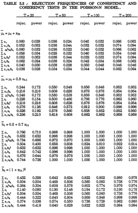
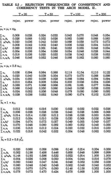
The consequences of specification error call for a careful evaluation of at least the first four conditional moments, and for an assessment of whether there may be substantial loss of information due to incorrect distributional assumptions. Chapters 5 and 6 are devoted to this task. In Chapter 5 we derive general diagnostic tests which do not use information external to the model. To evaluate the first two moments we produce tests of the coherency of the
information of the two moments, and a more general class of tests which we call consistency tests can be derived from residual analysis of both the mean and the variance equations. This class includes the tests of coherency of
information and is related to other procedures in the literature, mainly those of Hausman [1978], White [1980a], Pagan and Hall [1983], Ruud [1984], Cameron and Trivedi [1985], and Breusch and Godfrey [1986]. The distribution of
consistency test-statistics is derived under the null hypothesis and sequences of local parametric alternatives by relating this family of tests to conditional
moment tests (Newey [1985a, 1985b], Tauchen [1985]), and the tests can be computed from the coefficient of determination of a double-length auxiliary regression with the residuals of the two equations as dependent variables. An example is given by applying some simple tests to the GARCH specification for foreign exchange rates of Engle and Bollerslev [1986]. To evaluate the
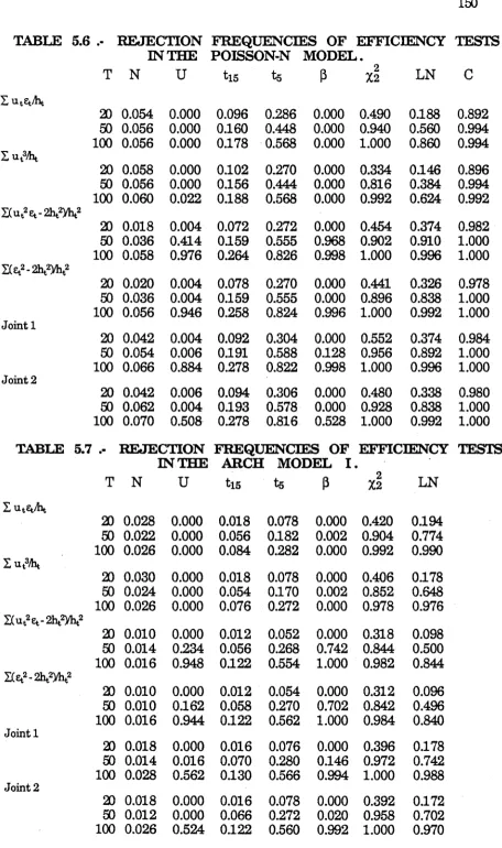
specification of moments of order third and higher, we develop a general class of tests which we call efficiency tests. Efficiency tests are also based on the analysis of the residuals, and the distribution of the efficiency test-statistics is also derived by relating them to conditional moment tests.
desirable directions. The LM test for variable additions (Breusch and Pagan [1980], Engle [1982b, 1984], Pagan [1984a]) in the mean or variance equations is shown to be a consistency test by suitable choice of the moment restrictions. The results of Engle [1982b] are extended to the case of a non-diagonal covariance matrix, and the principle is used to generalize some typical
departures considered in applied work to a heteroskedastic setup. We consider testing for autocorrelation, lag orders and common factors in both the mean and variance equations; testing for structural breaks (Chow [I960]) and
prediction error tests (Salkever [1976], Pagan and Nicholls [1984]); and testing for weak and strong exogeneity (Engle et al [1983], Wu [1973], Hausman [1978], Geweke [1978]). As to testing the higher order moments, the normality test of Jarque and Bera [1980] against the Pearson family is generalized to
heteroskedastic models and shown to be an efficiency test by suitable choice of the conditional moment restrictions.
The developments mentioned above constitute a more complete theoretical body of inferential procedures than has been provided so far in the literature on heteroskedastic models, and in order to have some means to assess the
performance in small to moderate samples of the asymptotic approximations derived, some Monte Carlo experiments are reported at the end of each of Chapters 2 to 6 .
Our next task is to try to cover a wider range of situations, and we proceed to generalize the results obtained so far. This is the objective of the four
chapters which constitute the second part of the Thesis. In these chapters the estimation and evaluation framework of the first part of the Thesis is adapted to more general situations, and since the generalizations are made in different directions there is not a sequential path to the reading of these four chapters.
parametric risk measures, derive tests for risk effects, and classify parametric risk models in terms of the relationship between the risk measure and the variables in the model. When the risk term is a function of the conditional variance of the dependent variable we term the model a y-risk model (as the ARCH-M model of Engle et al [1987]). The regularity conditions and
factorization of the likelihood are reconsidered in this framework, and it is seen that the consistency and efficiency tests derived in Chapters 5 and 6 apply
directly to y-risk models. The risk premia model of Engle et al [1987] is
analyzed as an illustration. When the risk measure is a parametric function of the conditioning variables we term the model an x-risk model (Hansen and Hodrick [1983]). Inference may be conducted on x-risk models from the joint likelihood, or from the conditional likelihood using a two-stage approach (Pagan [1984b, 1986]). Two-stage estimators are derived and their properties are analyzed, and the efficiency and consistency tests are extended to the two- stage procedure by taking into account the additional source of randomness introduced by the extraneous estimates obtained in the first stage.
In Chapter 8 we consider varying coefficients in the conditional mean. The coefficients may vary deterministically (Belsley [1974a, 1974b]), randomly (Swamy [1971]), or they may evolve randomly (Nicholls and Pagan [1985]). We discuss the conditions under which the results available for homoskedastic models extend to models with implicit sources of heteroskedasticity, and the estimation and evaluation procedures of Chapters 2 to 6 are easily generalized because the likelihood has been cast in state space form from the beginning. Further tests for parameter stability are derived which generalize well known results in homoskedastic models (e.g. Breusch and Pagan [1979], Nicholls and Quinn [1982]), and an evolving coefficient model for the joint parameters of the conditional and marginal models is proposed to represent a learning
model must introduce new information in stages, and LM tests for superexogeneity are derived.
In many cases researchers are interested in modelling more than one variable, and we face the task of generalizing our results to a multivariate framework in Chapter 9 . The model is interpreted as a system including mean, variance and covariance equations with (possibly) cross-equation restrictions, and we extend the principle of extracting information separately from orthogonality conditions and of combining the information in matrix weighted averages. The likelihood function of the multivariate normal heteroskedastic model can be locally factorized and the consistency and efficiency tests are generalized to evaluate the model, using vectorizations of the higher order moments.
Once the move has been made to incorporate the second moment into the modelling process, the question arises as to the possibility of considering higher order moments as well. In Chapter 10 we explore this situation by viewing the problem as a generalization of extracting information from the variance under heteroskedasticity: each moment provides an additional equation to the system introducing the potential to improve efficiency in
estimation, and we can extract the information from orthogonality conditions. To motivate this exploration we use the two-moment case when the distribution is not symmetric and the estimators may not be combined by simple matrix weighted averages. We use a modified version of the variance equation that contains only the information not already contributed by the mean, and with this we recover the asymptotic independence between the separate estimators. This approach is then generalized to produce a sequential search for
equations is solved by the use of residuals from the mean equation. When the conditional distribution is symmetric this raises no further problems, but when the distribution is not symmetric, substituting innovations by residuals
introduces a new source of uncertainty which must be accounted for. The tests for coherency of information are generalized and constitute an integral part of the search for information in higher order moments.
CHAPTER 2
THE BASIC MODEL
This Chapter is a reference for the main core of the Thesis contained in Chapters 3 to 6 . The model and notation are presented in section § 2.1 and the basic assumptions discussed in section § 2.2 . It is not our purpose to weaken the set of assumptions to the last consequence, nor do we want to make such assumptions at an excessively high level. We follow Hansen [1982] and White and Domowitz [1984] and relate their hypotheses to the specific case of
heteroskedastic models. In section § 2.3 we analyze some of the more
important particular cases in the literature. The Chapter concludes with the presentation of the experimental design for the Monte Carlo evidence that will be discussed in Chapters 3 to 6 .
§2.1 Basic model and notation
We start from the relation between a (scalar) variable Y and a vector of variables X* . The primitive theoretical proposition is that Y is a function of X* , Y = Y(X*) . The variables correspond to measurable and observable concepts and are thus related to specific time periods or units. For the t-th
*
period, Y and X* are represented by yt and xt , respectively. Throughout the Thesis we place the emphasis on time-series models, but many of the results we derive apply as well to cross-section models and to panel data. However, some of the concepts introduced would not make sense in a cross- section framework and would require modification.
g * g * * *
Yt = a{ ys , ys+i y t ) , and \ = a{ xs , xg+1 xt } ,
where for any set of observations A , a(A) represents the corresponding a- algebra (White [1984], Spanos [1986]). We use Yt = YT° and = Xt “*° to designate the past information sets of Y and X* respectively, up to and including period t .
*
The data generating process (DGP henceforth) for ( y t, xt ) is the time- dependent probability mechanism that underlies the stochastic structure of the variables (see Hendry and Richard [1982,1983]), and is given by the joint
probability density function (pdf) conditional on past information (!) . This joint DGP can always be factorized as
D ( yt , xt I 9 t) = D ( yt I CTt) D ( ^ I 9 t ) ,
* *
where 9 t = v ( Yt-i U Xt l ) is the past information set, and y t = a (Yt.i U Xt ) =
*
a ( 9 t U x t )is the conditioning information set, and we have that 9t c • Corresponding to the primitive theoretical proposition Y = Y (X*) , our interest is to construct a statistical model for the conditional DGP D( yt I t ). This constitutes the conditional model. At the extreme of generality we may build a fully non-parametric conditional model, and at the extreme of
specificity we can construct a fully parametric one. In between these two extremes we have the semi-parametric alternative in which part of the
conditional model is characterized by a finite-dimensional parameter set and part by an infinite-dimensional one. In the literature on heteroskedastic models Amemiya [1973,1977], Jobson and Fuller [1980], Engle [1982a], and Bollerslev [1986] are examples of parametric models, Fuller and Rao [1978], White [1980b], Carroll [1982], Carroll and Ruppert [1982b], Amemiya [1983],
Cragg [1983], and Robinson [1987] are examples of semi-parametric specifications, and Hall and Carroll [1987] analyze a fully non-parametric
model. Our approach is mainly parametric though we consider the possibility of specifying only a few conditional moments which is itself a semi-parametric proposition. Also in Chapter 3 we briefly review some semi-parametric
approaches to inference and explore the possibilities of mixed parametric/semi- par ametric strategies.
A random variable is fully characterized by its distribution or its
characteristic function. Our weakest proposition is a partial description of the characteristic function by the parametric specification of the first two moments of the conditional DGP. The conditional mean is characterized by a k-
dimensional parameter vector ß , ß s B C Rk , that is,
E [ yt I 3^ 1 = Pt = M-t (ß) = M-t ( ß ; ^ t ) •
The information set 2T t and the parameter vector ß will not be shown as explicit arguments unless necessary. For ease of reference to the most common case in which pt is linear in ß we denote
xt = xt (ß) = xt ( ß;3rt) = “ “ , öß
which does not depend on ß in the linear case. The conditional variance is characterized by the p-dimensional parameter vector 9 , 0 e @ C R p , a s i n
Var [ yt l DM = ht = ht (0) = ht ( 0 \& t).
The class of models which is of our particular interest is that in which pt and ht have common parameters. To allow for this we let p > k and introduce the vector a , a e C Rp-k , such that 0 may be partitioned as 0 = ( ß ', of )'. In most cases 0 = B x Qx , but this need not be the case. Thus p is the total number of parameters for the two conditional moments. Also for ease of reference to the most common case, denoted the linear-in-a model , in which ht is a linear function in a , we define
3ht 0a ’
so that when ht is linear-in-a we have ht = a , where zt = zt(ß) in general. The other partial derivative of ht is
wt = wt (9) = wt ( 9 ;DTt ) = , -(2)
dß and wt and zt are stacked into
St = st (9) = st ( 9 jSFt) = “~ = •
The parameter space @ and/or the function ht and its variable arguments in J t need to incorporate restrictions to ensure ht > 0 for all t . This can be achieved if ht = h(^t) , where £t = ( 9 jSFt) > and h(^) > 0 V % , which generalizes the formulation of Breusch and Pagan [1979]. For example, Harvey [1976], Hausman et al [1984], Gourieroux et al [1984b] and Geweke [1986a] choose h(-) = exp(-) . Other functional forms may require restrictions to be imposed on the parameter space (mainly on Ci ), but for most well known variance
specifications such restrictions can be enforced through reparameterization of the model. In linear-in-a models we assume that zt > 0 (2) , so that
reparameterizing in terms of a* = a 1/2 ensures positivity.
In parallel to the specification of the conditional moments pt and ht we have the corresponding sequences of innovations. The innovations in the conditional mean of yt are
ut = ut (ß) = yt - E [ yt 12Tt ] = yt - P t, - (3) and the innovations in the conditional variance of yt are
et = et (9) = u? - E [ ut I ^ t 1 = ut - ht . - (4) The joint modelling of pt and ht requires new information to accumulate on both moments and this is reflected in the two sets of innovations ut and et . In
(2) We make the convention that scalar functions and expressions referred to vectors apply element
other words, there are two distinct, though possibly related, relationships
underlying the heteroskedastic model. From (3) we derive the usual regression function
yt = M-t (ß) + Ut , - (5)
which will be referred to as the mean equation . And from (4) we obtain the second relation
ut = ht ( ß , a ) + 8t = ht (0) + 8t , - (6) which will be referred to as the variance equation . The disturbances ut and St in these equations are not added errors', but are derived from the proposed model for the DGP (see Hendry and Richard [1982,1983], Spanos [1986]).
In Chapter 3 we gain insight into the problem of inference in
heteroskedastic models by treating the mean and variance equations as a set of seemingly unrelated regression equations (SURE, Zellner [1962]). Let gt = gt(9) = gt (9 ) = ( M-t > ht )', % = ( yt , ut )', and Ut = ( ut , et )'. The two-equation
system is given by
Tit = gt (9) + u t , - (7)
and has conditional covariance matrix
Xt = var[utlD rt] = E [ u t Ut, i y t ] = ^
Jt
^* 2 *
where A t = E [ ( yt - |it )3 1 7 1 ] , Kt = var [ £t I 7 1 ] = k,. - ht , and Kt =
*
E [ ( yt - Mt )4 I 7 1 ] » and of course /&t, ^ 6 ^ t (3) • The parameterization of these
higher order moments will be explicitly introduced when required. When the conditional distribution is symmetric we have that At = 0 and Zt is diagonal.
O ur strongest proposition is the complete param etric specification of the conditional DGP,
D ( yt I 2Tt) = f ( y t I SFt; 9 , 7C),
where f(-) is a pdf and k is the vector of (possible) additional param eters in
moments of order higher th an two. In this case we use the likelihood function
£ ( 0 , t u)
r
tI lf Cy t i a v. e, * )
_t=i
f ( yo I y o ; 9, k ) , - (8)
where f ( yo I 7 o ; 9, ft ) represents the information from the initial conditions yo . The corresponding log-likelihood is given by
T
i ( 9, Jt) = T"1 £ log f ( yt I 7 t ; 9. ft ) , t=l
where the conventions of normalizing by sample size, neglecting constants, and the assum ption th a t the term T'1 log f (yo I 3T o ; 9, k ) has no asymptotic
effect for inferences on 9 and k , are utilized. The subvector of the score for 9 is
9 i( 9 ,7i) ^ d log f (yt l y t ; 9, x ) I , ' fdß( 9, tu )>
do( 9 ,7C)
99 t=l t=l da( 9, k )
in obvious notation and partition, and the information subm atrix for 9 is dee( 9, k ) = - E "92i ( 9,
k ) (iJßß( 9, 7U) dßa( 9» ft )")
dQdQ' " [üaß( 9. Jt ) <Jact( 9, 7C )j
The most common full param etric model is the normal model which assum es conditional norm ality, th a t is,
yt l 7 t ~ N [ p t , h t ] ,
and it has been used successfully in heteroskedastic econometric models in many cases. See for example Engle [l 982a,1983], Weiss [1984], Domowitz and Hakkio [1985], Bollerslev [1986], Diebold and Nerlove [1986], and Engle et al
alia . O ther distributions th a t have played an im portant role in the subject either theoretically or empirically and th a t will receive mention in this Thesis are the t-distribution (Bollerslev [1985], and Engle and Bollerslev [1986]), the gamma distribution (Amemiya [1973]), and the Poisson distribution and other distributions compounded with the Poisson (Hausman et al [1984]),
Gourieroux et al [1984b], and Cameron and Trivedi [1985,1986]). For some specific purposes other more general distributions such as the Pearson family (Kendall and S tu art [1968]) will be used as well.
Since the normal model will play an im portant role in our analysis, it is convenient to present the likelihood, score and information m atrix for this case (see Engle [1982a]). These are given by
i(8) = - \ T-i X ht - I T-l X hi1 u? , - (10)
t=l t=lt=l
de(0) = T-1 Yj ht1 xt ut + I T-1 Y h ~t2 st et
t=l t=l
= T-1 x' a-1 u + 1 T"1 S' a-2 8
T-1 G' I-1 u , - (11a)
dp(0) = T*1 Y ^t1 xt ut + t? T-1 Y ht2 wt et
t=l t=l
= T-i X'Q-i u + \ T*1 W Q-2 8 , -(lib )
da(0) = I T-1X ht2 Zt et = \ T-1 Z' Q-2 e , T
- ( 1 1 c ) t=l
m = E [ T-1 G' Z-1 G ] = E
/ T-1X'£2-1X + | T-iW'Q-zw ^ |t-!Z'Q-2W
|x -iW 'Q -2Z^ | t-iZ'Q-2Z
(12)
where xt = ( xt', 0 ) ', y = ( y i ...y r ) ' , H = ( H i M - t)' . u = ( u i u t)' ,
h = ( h i h r ) ' , e = ( e i,..., 6t) ', X = ( x i xt)' , X = ( x i x t)' = ( X , 0 ) , W = ( w i wT ) ' , Z = ( z 1 ,...,z T )/ , S = ( S i s t)' = ( W , Z ) , rj = ( y7, u2' )' , g = ( |I ' , h ' )' , X) = ( u ' , s' )' , a = diag { hi,...,hT } , A = diag { } ,
K = diag { , G W z ) z Q
A K . In (9) - (12) we have used the properties of the normal distribution th a t A = 0 and K = 2 Q2 , and the functions depend only on 9 because the normal distribution is completely characterized by its first two moments. For this reason we have also deleted the '90' subscript from the inform ation matrix.
§ 2.2 Assumptions
The previous section gives form to the model and produces our fundam ental 'correct specification' assum ption
(C|0) The conditional mean o f yt is |it(ßo) = E [ yt I IFtl > its conditional
variance is ht (0o) = Var [ yt I IF 11 > and the third and fourth moments
are given hy /&t = E [ { yt - lit (ßo) }3 1 ] and k,. = E [ {yt - Jit (ßo) )4 1 ]
which exist and are finite conditional on 7 1 .
A full param etric alternative to (CiO) is
(C*07) y t l 3 ^ ~ N [ j i t ( ß o ) , h t ( 0 o ) ] .
O ther possibilities are the gamma, the Poisson, or Student's t
There are now available many powerful results to establish the asymptotic properties of estimators in nonlinear models under a variety of circumstances, see Jennrich [1969], Malinvaud [1970], Hannan [1971], Burguete et al [1982], Hansen [1982], White and Domowitz [1984], inter alia . The last two references are of particular interest and will allow us to establish the main asymptotic results under different conditions of heterogeneity and dependence of the processes involved. The generalized method of moments (GMM) theory of Hansen [1982] permits relatively mild memory restrictions for economic
variables in the form of ergodicity, and requires a degree of homogeneity which is fulfilled by strict stationarity. The general theory for nonlinear regression with dependent observations presented by White and Domowitz [1984] allows for more heterogeneity by strengthening the conditions on the memory of the
process to uniform or strong mixing of some given order. In line with this, our next assumption is
*
(CU) ( y t, xt ') is stationary and ergodic, or
*
( yt , xt ' ) is mixing with <j>(m) of size r/(2r -1), r > 1, or aim) of size
r/(r -1), r > 1 .
2 *
Note that ( ut , xt ' ) has the same heterogeneity and memory structure than *
( y t, xt ' ) e.g. Lemma 2.1 of White and Domowitz. This is important for the estimation of the variance equation. The parameter space is restricted by
(C|2) © is a compact suhspace of Rp and 0o is an interior point of © .
Not allowing 9o to lie on the boundary of the parameter space is required for a well-behaved (normal) asymptotic distribution of the estimators.
(0.3) fit and ht are measurable functions of 2Tt for all 9 e 0 , and are continuously differentiable of order 2 on 0 , uniformly in t .
Further, and ht and their first two derivatives with respect to 9
are bounded from above and ht is bounded away from zero almost everywhere in 0 , uniformly in t .
This assumption states the smoothness conditions which are characteristic of parametric work in heteroskedastic models in econometrics. Given this
smoothness and the compactness of © , boundedness relates to functions of moments of the variables which are generally assumed to hold (e.g. the convergence of T*1 X' X in the classical linear model). Positivity of the conditional variance typically imposes some restrictions on the parameter space 0 , as discussed in the previous section.
We must ensure the existence of the first few unconditional moments and also that we can take expectations of the likelihood function or other estimation criteria (quadratic in nature) over the parameter space. For this purpose we introduce
2
(Cl4) St = £t(9o)2 is uniformly (r + 5)-integrable r > 1, 5 > 0 , while
[ jLLt (ßo) - M-t (ß) l2 and [ ht (9o) - ht (9) ]2 are dominated by uniformly
(r + h)-integrable functions .
Note that the uniform integrability of St implies the existence of at least four moments of yt . The first two are usually assumed for mean models, and the last two are required for the proper estimation of the variance equation. Also observe that this imposes conditions on dynamic models which in general imply further restrictions on the parameter space 0 .
These assumptions are required to ensure the proper asymptotic behavior for the Hessians of the relevant criterion functions.
(Cl5) The matrix function of 9 given hy —— St “ 7 is dominated by
o0 o 6
uniformly r-integrable functions, r > 1 , and has finite expectation at
90 .
(Cl6) { Kt xt xt' - ht1 ut (ß) TT7 ) and { k^1 st st' - k*1 et (9) “ 7 } are
dp d0
dominated by uniformly r-integrable functions, r > 1 .
Observe that (Cl5) is sufficient for the same condition to apply separately to h't1 xt xt' and iq1 st st' .
Finally, identifiability is ensured by means of
(Cl7) Var [ T - ^ X' Q_1 u ] = E [ T-1 X' Or1 X ] and Var [T-1/2 G' Z*1 u ] =
E [ T-1 G' Z-1 G ] are uniformly positive definite in an open neighborhood of 0o.
The equalities in (Cl7) are obtained using iterated expectations. In other words, (Cl7) ensures the identifiability of ßo in the mean equation, and that of 9o in the two-equation system. Because the mean equation does not contain information about ao , then given ß , this vector must be identifiable in the variance
equation. Therefore (Cl7) implies that Var[ T*1/2 Z' K'1 s ] = E [ T*1 Z' K*1 Z ] is uniformly positive definite in an open neighborhood of 0o .
In Chapter 3 we make repeated use of Theorems 3.1 and 3.2 of White and Domowitz, and Theorems 2.1 and 3.1 of Hansen. A summary of these results can be stated as
T h eo rem 2.1.- Suppose a parameter vector X e A C IRn is to be estimated by
x =
min \ |f ( xy A T v ( WT
where \\f (X) = T*1 £ \\rt (X), E [ \\rt (Xo) ] = 0 , and At —> S { T \j/(Xo) \|/(Xo)'}(4), t=l
where Xo is the true value of X . Assume th a t the regularity conditions of H ansen and/or White and Domowitz are fulfilled for this problem. Then
t^ u -Xo) A f j [ o , v ( £ ) ] , where
v d ) = [ e ( 9 ^ / o) ) g { 9 ^ ) } ] 4 .
dX dX
Proof: See Theorems 3.1 and 3.2 of White and Domowitz and Theorems 2.1 and
3.1 of H ansen. Q
A unified treatm ent of both types of estimators is considered by Burguete et al [1982], and Chamberlain [1987] discusses the selection of the optimal
weighting matrix. In order to avoid later repetition we establish here the sufficiency of the assumptions (ClO) - (Ci7) for the application of these results to our specific problem.
P r o p o s itio n 2.2.- Suppose the mean equation in (5), or the variance equation in (6) , or both equations jointly as in (7), are to be estim ated respectively by
minp { u ' Q-1 u }, mine { s' K-1 e }, or min© { n' It1 u } , where Q. , K and X are given. Let (Al) - (A9) denote Assumptions 1 to 9 of White and Domowitz [1984]. Then (ClO) - (Cl7) are sufficient for (Al) - (A9).
Proof: (Ci2) and (Ci3) => (Al) and (A5); (Ci4) => (A 2); (ClO) => (A3); (Ci7) => (A4) and (A9) ; the m artingale assumption in (ClO) with Exercise 5.26 of White [1984] ensure th a t (Cl7) also implies (A7) ; (Cl5) => (A6) ; and (Cl6) => (A8). The mixing conditions of Theorems 3.1 and 3.2 of White and Domowitz are guaranteed by (Cil), and therefore we can readily apply these results to generalized least squares (GLS) estimation of the equations in (5) - (7).
For any random sequence XT we define 6 ( XT} = lim E [XT ], provided such limit exists.
P ro p o sitio n 2.3.- Suppose the mean equation in (5), or the variance equation in (6), or both equations jointly as in (7) , are to be estimated by the GMM method w ith orthogonality conditions given by equating to zero the param etric
functions T*1 X' Q_1 u , T*1 S' K*1 e , or T'1 G' £4 u , respectively , where O. , K and £ are given. Let (A2.1) - (A2.5) denote Assumptions 2.1 - 2.5, and (A3.1) - (A3.6) denote assum ptions 3.1 - 3.6 of H ansen [1982]. Then (ClO) - (Cl 7) are sufficient for (A2.1) - (A2.5) and also for (A3.1) - (A3.6).
Proof: (CU) => (A2.1) and (A3.1); (Cl2) and (Cl3) => (A2.2), (A2.3), (A3.2), and (A3.3). The m artingale difference assumption in (Cl0) together with (Cl5) and (Ci7) are sufficient for (A2.4), (A3.4) and (A3.5), by Theorem 5.24 of White [1984]. Since there are as many orthogonality conditions as param eters in all three cases, (A2.5) and (A3.6) are trivially satisfied. Finally, note th a t for Theorem 2.1 of H ansen condition (i) is guaranteed by (Ci5) and his Lemma 3.1, (ii) is ensured by (Ci2), and the identifiability condition in (iii) is fulfilled in view of (Cl7). Therefore, we can also readily apply Theorems 2.1 and 3.1 of H ansen to the heteroskedastic setting under (ClO) - (Cl7).
The GLS estim ators of White and Domowitz and the GMM estim ator of H ansen cannot make claims of efficiency other th an in relation to the
orthogonality conditions involved(6) . Such relative efficiency follows trivially in this case from Theorem 3.2 of H ansen and also from Chamberlain [1987]
because the num ber of orthogonality conditions in Proposition 2.3 equals the num ber of param eters, and hence the definition of a weighting m atrix is
superfluous. U nder some circumstances, however, stronger efficiency claims can be made. This generally entails the knowledge of the form of the
conditional DGP up to the param eter vector 9 , and for full efficiency in the Cramer-Rao sense in this context we will require the additional assum ption
*
(Cl8) The variables ^ are weakly exogenous for 9 in the sense o f Engle, Hendry and Richard [1983] .
This ensures that the conditional likelihood in (8) contains all the relevant information about 9 .
§ 2.3 Some special cases
In this section we present some particular cases of heteroskedastic models which have been studied and applied in the literature. Subsection § 2.3.1
considers models in which ht is not a function of ß , while the remaining subsections deal with cases in which ht is parameterized as a function of ß .
§ 2.3.1 Simple heteroskedasticity
In cross-section models it may be too restrictive to assume that all units can be represented by a fixed parameter set. Hildreth and Houck [1968] and Swamy [1971] have proposed a more general model in which the coefficients vary randomly across units as drawings from a common parent distribution. This has led to the random coefficients model which results in a specific
heteroskedastic pattern. An alternative is to allow for changing variances and to try to model these changes as functions of other observables. In time series models confusion in the relationships between nominal and real measures induces heteroskedasticity (see Theil [1971]), and the same happens in general if the ß coefficients evolve stochastically through time. These are cases of the simple heteroskedastic model which is defined when
ht = ht ( a ; CT t ),
follows that the maximum likelihood estimators (MLE's) of ß and a are asymptotically independent.
The most common form given to ht has been a linear one, ht = zt a , where zt e & t , (Amemiya [1977], Pagan [1984a], Pagan and Hall [1983], inter alia ). Other possible models include the simple quadratic ht = (zt'a)2 (Glejser [1969]), and the multiplicative ht = exp {zt'a} (Harvey [1976]). All these are encompassed by the parameterization of Breusch and Pagan [1979] in which ht = h(zt'a) , for some continuous function h(-) taking positive values only. A constant is usually included in zt so that homoskedasticity is nested within this model. If zt is strongly exogenous no further conditions are required in general for the existence of moments. But if zt is weakly, but not strongly, exogenous so that zt is Granger-caused by yt (see Granger [1969], Engle et al
[1983]), restrictions may be needed on the parameter space for the existence of fourth order moments. Even a simple model like this can produce a very complicated dynamic structure involving both the conditional mean and the conditional variance, and these dynamics will certainly have to be non
explosive for the existence of fourth order moments. Dominance conditions are trivially satisfied if ht and pt are linear. If this is not the case, some structure on the functions pt (*) and ht (•) may be required.
We must also mention in this section the attempts in the literature to allow for heteroskedasticity without going through the burden of specifying the conditional variance. This has led to semi-parametric models in which ht is only specified as
h t = h t (
y
t ) .is put forward other than the variables involved as arguments, and maybe some ranking relations.
§ 2.3.2 Amemiya Model
One of the earliest references to a model in which the heteroskedasticity is made dependent upon ß is the Prais and Houthakker [1955] study of family budgets (see also Theil [1951]). There they propose a cross-section model in which the variance is proportional to the square of the mean,
ht = a (it ,
and therefore ht = ht ( ß, a ). They did not capitalize, however, on the
information provided by the variance. Amemiya [1973] considered this model in a likelihood framework and proved that the GLS estimator of ß would be inefficient if yt was distributed normally or log-normally conditional on 7 1 > thus showing the potential importance of variance information. He also proved that if yt I y t ~ T (a ,a_1 p t), then GLS for ß would be fully efficient.
This model is clearly linear-in-a , and from (1) and (2) we have
2
zt — M-t > and
wt = 2 a pt xt ,
so that using (12) we have under conditional normality T
%a(e) = a - i E [ T - i £ n i1xt ] > t=l
which will be nonzero in general. Therefore there is asymptotic dependence between the MLE's of ß and a in the Amemiya model.
*
nature of xt . Positivity is ensured by a > 0 and this can be implicitly
incorporated parameterizing in terms of a2 i.e. ht = a 2 pt • But the parameter space has to be restricted to meet the moment conditions when dynamics are allowed in the conditional mean. Dominance conditions, on the other hand, are straightforward when pt is linear.
Homoskedasticity is not nested within the proposition ht = a pt » but it can be incorporated with the obvious generalization to ht = ao + ai pt , where ao > 0 and ai > 0 , so that homoskedasticity obtains when ai = 0 (Jobson and Fuller [1980]). A simple further generalization to other functions of jit is
ht = ao + oci hi (pt ; a2) - (13)
where hi(-) is a non-negative function of pt and must obey some smoothness conditions to satisfy the regularity requirements.
§ 2.3.3 The Poisson and Poisson-type models
There are many economic examples in which the dependent variable is discrete rather than continuous (e.g. Maddala [1983], McFadden [1984]). In many instances discrete economic variables can be characterized as Poisson or Poisson compounded processes. Some examples are Chatfield et al [1966], Chatfield and Goodhardt [1970] and Ehrenberg [1972] in analyzing purchasing behavior, and Hausman et al [1984] in the study of the relationship between patents and R&D expenditure, while Cameron and Trivedi [1985,1986] survey the literature and propose diagnostic tests for these models.
The mean and variance of a Poisson variate are equal and therefore
Pt = P t ( ß ; * t ) = ht . -(14)
dependent variable and its importance in modelling count data. Also observe that there are no a parameters in (14) and so p = k and 9 = ß .
Rather than restricting the parameter space to ensure ht > 0 (and also P t > 0 in this case) Hausman et al [1984] and Gourieroux et al [1984b] argue for a parameterization that implicitly incorporates positivity, and they suggest
* *
p t = h t = exp { X t ' ß } , which implies a null zt and x t = w t = P t x t . Dominance conditions are ensured by the compactness of B with this proposition. The required moment conditions and whether the parameter space needs to be further restricted depends on the dynamic characteristics of the model.
A more general version of the Poisson model compounds this distribution with a random distributional parameter. Hausman et al have introduced random effects by these means, while Gourieroux et al have allowed for specification error. A gamma-distributed parameter has led to negative binomial models (see also Ehrenberg [1972]). Such extension of the Poisson model allows for overdispersion ( ht > p t) and produces a natural diagnostic for the Poisson model. Cameron and Trivedi [1985] propose alternative
regression-based tests for over-and under-dispersion parameterizing the conditional variance under the alternative hypothesis as
ht =• pt + a hi (pt ),
for some positive function hi . Then a < 0 (a > 0) results in under- (over-) dispersion and a = 0 represents the Poisson null hypothesis.
Using Poisson characteristics with a continuous dependent variable results in Poisson-type models in which the central issue is the moment relationship in (14). Cameron and Trivedi [1985] and also Pagan and Sabau [1987a] consider the model
and the former authors consider alternative assumptions by specifying the first four moments. Here again the fulfillment of the assumptions in § 2.2 depends on the nature of pt and its variable arguments in 7 1.
§ 2.3.4 The ARCH class of models
Engle [1982a] proposed the ARCH model to account for inflation uncertainty, and subsequently this model has been successfully applied to study many financial variables (see Engle and Bollerslev [1986] for a survey of applications). The conditional variance of an ARCH process depends on past information, drawing a clear distinction between the conditional and the unconditional second moment of the variable under study. The (linear) ARCH(q) process is characterized by
. A 2 ,
ht = cco + 2, ai ut-j = zt <*, j=l
2 2
where zt = (1 , ut-i ut-q )' and a = ( ao , a i ,..., a q )' , and therefore has a q
linear-in-a structure. The derivative with respect to ß is wt = - 2 £ ut-j xt.j . j=l
The positivity constraint requires ao > 0 and aj > 0 , j = l,...,q , which may be implicitly incorporated by parameterization in terms of the af . An alternative approach has been to restrict the lag structure to reduce the number of
parameters and hence the probability of obtaining negative values. Although this procedure does not formally exclude negative estimates it has been
successfully applied (see Engle [1982a, 1983], Engle et al [1987]).
The moment structure of the ARCH(q) was analyzed by Engle for some cases, and Milhoj [1985] has produced general results. For wide-sense
q
stationarity we require ao > 0 and £ ccj < 1 (Theorem 1 of Milhoj), and then
q j=l
E [ ht ] = ao [ 1 - I aj T1 . The condition for the existence of fourth order j=l
II bi+j + bi_j II , an d bi = for 1 < i < q a n d bi = 0 otherw ise. T hus for
ex am p le for th e A R C H (l) th e condition is a? < 1/3 (Theorem 3 of M ilhoj). The ARCH(q) im plies a lep to k u rtic d istrib u tio n for y t , an d th is is one of its
a ttra c tiv e fe a tu re s for m odelling in te re s t ra te s , exchange ra te s , in fla tio n , stock p rices a n d o th e r fin an cial d a ta .
A n o th er in te re s tin g asp ect of th e ARCH m odel is t h a t <)aß = 0 u n d e r conditional n o rm ality a n d so th e ML e stim ate s of a an d ß a re asy m p to tically in d e p e n d e n t (E ngle [1982a]). T hus alth o u g h th e conditional v a ria n ce is a fu n ctio n of ß th ro u g h th e presence of ut-j , th e ARCH m odel re ta in s a sto ch astic s tru c tu re w hich is sim ila r in several aspects to th e sim ple h e te ro s k e d a stic m odel.
T he v arian ce m em ory of a n AB,CH(q) dies a fte r q periods a n d th is led B ollerslev [1986] to p u t forw ard th e G A RCH (qi,q2) process whose conditional v a ria n c e is
o r
bt - OCo + ^ ctj ht-j + ^ ttq-L+j u t-j >
j= l j= l
2
oci(L) h t = oco + 0C2(L) u t ,
- (15a)
- (15.b)
qi 02
w h ere L is th e lag o p erato r, oti(L) = 1 - X <*j LJ , an d 0C2(L) = X ocq +j L3 * for
j=l j=f
q2 > 0 . The boun d ed n ess of ht aw ay from zero still req u ire s oco > 0 an d (Xj > 0
for j > 0 , but- since (15) allow s for a long m em ory w ith a m ore p arsim o n io u s p a ra m e te riz a tio n th a n th e sim ple ARCH, it is also less d e m a n d in g in te rm s of ach iev in g p o sitiv ity in estim atio n . T he conditional v a ria n ce is n o t lin e a r-in -a in th e GAJRCH m odel.
B ollerslev provided th e n ecessary a n d sufficient conditions for w ide-sense s ta tio n a rity of th e GA RCH (qi,q2) process, w hich is th a t <xi(l) - 0C2G ) > 0 , or
qi+02
eq u iv alen tly th a t X ocj < 1 . He also gave th e n ecessary an d sufficient j= l
conditions for the existence of 2m-th order moments in the GARCH(1,1), and
2 2
in particular for the fourth moment we require that ai + 2 oq 0C2 + 3 ct2 < 1 , and similar conditions may be established for higher order processes following the
2
lines of Milhoj [1985] in obtaining the autocorrelation structure for ut . There is a close resemblance of the GARCH variance specification to ARMA models for the mean of a process. This is better appreciated by
substituting the variance equation (6) in (15b) to get
2
<xi2(L) ut = ao + ai(L) et , - (16)
where a i2(L) = oqCL) - 0C2CL) . Because of this similarity Bollerslev suggested the use of the autocorrelation and partial autocorrelation functions of ut as tools for model identification (see also MacLeod and Li [1983]). The et follow a heteroskedastic pattern and have changing support (see Engle and Bollerslev [1986]), but nevertheless Bollerslev's suggestion is entirely appropriate if fourth order moments exist because then et is unconditionally homoskedastic. An interesting alternative for model identification which is also valid in these circumstances is the Hannan and Rissanen [1982] procedure with some information criterion such as AIC (Akaike [1974]) or BIC (Schwarz [1978], see
also Geweke and Meese [1981]), and the advantage of such procedure is that it relies more on direct analytical results and less on visual inspection and subjective judgement.
We assume that the polynomials oci(L) and 0C2(L) do not have any
common factors. The wide-sense stationarity and positivity conditions ensure the invertibility of cci(L) and OC12 (L). Thus solving (16) for ut we obtain
2
u t = a i2(l)'1 oto + a i2(L)-1 ai(L) et ,
2
ht = ai(l)-1 ao + ai(L)*1 a2(L) ut ,
which expresses the GARCH(qi,q2) as an ARCH(«0. Thus the normal GARCH
process is also leptokurtic, and Bollerslev [1985] and also Engle and Bollerslev [1986] have proposed the use of the conditional t-distribution for fatter tails. Similarly, the block-diagonality of the information matrix of the normal ARCH extends to the normal GARCH.
ARMA models provide a rational approximation to the undeterministic component of Wold's decomposition of wide-sense stationary time series. Diebold [1986a] has argued that GARCH models may play a similar role in modelling conditional variances with time series data, and this suggestion is already implicit in Engle's [1982a] paper. Diebold argues that the
undeterministic component of wide-sense stationary series allows for a
changing conditional variance and hence GARCH processes are not excluded. But the power of the GARCH parameterization as an approximation to many heteroskedastic patterns is better understood from its ARMA form: if yt possesses fourth order moments then ut is wide-sense stationary and (16) provides a rational approximation to to its undeterministic component, while its changing conditional mean is ht = E [ ut I t ] •
Our main concern in econometric modelling is to construct statistical models of economic propositions. ARMA models are atheoretical propositions in general and from the previous argument the same could be said about GARCH models for the conditional variance. What is important about these models is that they permit us to make statistical propositions even in the
absence of a priori knowledge. As theory says more about the second moment we expect a movement towards a mixture of the different models presented in this section. Dependence of ht on jit and exogenous variables may represent the theoretical propositions about the variance, while a GARCH component can represent the dynamics in ht . This is the variance analogy of transfer