Essays on Non-Gaussian Time Series Analysis

(1)

Essays on Non-Gaussian Time Series Analysis

Peter Julian Cayton

December 2017

A thesis submitted for the degree of Doctor of Philosophy

of the Australian National University

c

Copyright by Peter Julian Cayton 2017

(2)

(3)

Declaration

I hereby declare that the work in this thesis is my own work except where otherwise stated. Part

of this thesis is based on joint research with my supervisor Dr Kin-Yip Ho.

(4)

Acknowledgements

This thesis is based on my three-and-a-half-year PhD program, funded by the University of the

Philippines (UP) Faculty Development Program - Foreign Doctoral Studies Fellowship and by the

Research School of Finance, Actuarial Studies, and Statistics (RSFAS) of the Australian National

University (ANU). During this period, I have been helped by many individuals and institutions. I

would like to express my gratitude to those who made this thesis possible.

Firstly, I would like to express my deepest thanks to my supervisory panel, Dr Kin-Yip Ho,

Dr Dennis Mapa, and Dr Yanlin Shi, for their encouragement from the very beginning of this

research, as well as their patience and support throughout the thesis work. I particularly thank

Dr Kin-Yip Ho for the guidance on all stages of my PhD study. His enthusiastic support made

my PhD experience productive. His perseverance and patience in supervision has been crucial to

completing my thesis. His counsel is invaluable for the direction of my PhD study and on my

career moving forward. My time as his research assistant opened my potential in doing further

research in finance and statistics. I sincerely thank Dr Dennis Mapa for opening opportunities for

me to disseminate my research in many avenues back home in the Philippines. He introduced me

to the field of financial econometrics and extreme value modelling in my undergraduate years. The

field has since been my research interest. I give my warm thanks to Dr Yanlin Shi, for his guidance

on writing the thesis and on engaging conversations about the directions of this thesis and of my

research direction. Throughout this PhD study, Dr Kin-Yip Ho, Dr Dennis Mapa, and Dr Yanlin

Shi have always been treating me as a colleague and friend, and I have learned a lot from them.

Stimulating conversations on research and on thoughts about life are of great value to me. They

have developed and supplemented my fervour for research which will further my academic career.

I would like to express my warmest gratitude to UP for their generous funding in the first three

years of my PhD studies through the Faculty Development Program Foreign Doctoral Studies

Fellowship. The fellowship generously provided for my living expenses and tuition costs for the

first three years and provided me a paid study leave throughout the PhD period. I would like to

extend my thanks to then UP President Alfredo Pascual, PhD and then Vice President for

Aca-demic Affairs Gisela Concepcion, PhD, then Vice President for Planning and Finance Lisa Grace

(5)

Dean Erniel Barrios, PhD and their staff for facilitating the conferment of the fellowship. I also

thank the current UP President Danilo Concepcion, PhD and Vice President for Academic Affairs

Maria Cynthia Rose Bautista, PhD, Vice President for Planning and Finance Joselito Florendo,

PhD, and UP Diliman Chancellor Michael Tan, PhD, and UP School of Statistics Dean Dennis

Mapa, PhD and their staff for continuing my fellowship until its expiration of funds last July 2017.

I also thank UP Diliman Chancellor Michael Tan, PhD, and School of Statistics Dean Dennis

Mapa, PhD for providing my paid study leave while pursuing my PhD studies in Australia.

I would also like to thank the warm faculty and staff of the UP School of Statistics for the great

times and friendships during my time in the Philippines. I would like to thank Assoc Prof Genelyn

Ma. Sarte who is a mother figure and an important psychological support in my time as instructor

in UP and during my PhD study in Australia. I also extend my thanks to my academic mother

dur-ing my MS (Statistics) program in UP and the incumbent National Statistician of the Philippines,

Dr Lisa Grace Bersales. Her guidance inspired me to pursue PhD studies overseas. I would like to

thank Dr Erniel Barrios who pushed much of the younger faculty like me to go out of the country

and pursue studies overseas with the promise of coming back to UP. Other faculty members that

I would like to thank are: Prof Manuel Albis, Ms Czarinne Antonio, Dr Josefina Almeda, Prof

Martin Borlongan, Dr Wendell Campano, Prof Therese Capistrano, Ms Charlene Celoso, Dr John

Carlo Daquis, Prof Francisco De Los Reyes, Prof John Eustaquio, Prof Iris Gauran, Prof Charlie

Labina, Dr Joseph Lansangan, Ms Jessa Lopez, Prof Michael Lucagbo, Dr Joselito Magadia, Prof

Angela Nalica, Dr Welfredo Patungan, Prof Joyce Punzalan, Mr Ruzzel Ragas, Mr Paolo Redondo,

Dr Reynaldo Rey, Ms Sabrina Romasoc, Mr Gian Roy, Dr Kevin Carl Santos, Prof Michael Van

Supranes, Dr Ana Maria Tabunda, Dr Jeffry Tejada, and Prof Stephen Jun Villejo. I would like

to thank the staff for their assistance with much of the clerical work that I had to do before and

during my PhD study: Rhodalizeil Tingco, Nancy Angala, Jose Jude C. Molina, May G. Garcia,

Emma A. Dublin, Evelyn B. Torres, Luzviminda Francisco, Edwin A. Ledesma, and Romulo M.

Niegas. I would like to thank and dedicate this thesis to Jaime Cabante, librarian of the School of

Statistics during my time there, now deceased.

My special thanks are also for the RSFAS for their generous funding throughout my PhD

pro-gram and providing a nurturing academic environment for my research. I would like to thank

RSFAS Interim Dean Steven Roberts, RSFAS Interim Director Stephen Sault, and PhD Statistics

and Actuarial Studies Convenor Dr Timothy Higgins for providing me with a fee-waiver scholarship

and a generous PhD allowance which facilitate my attendance to various conferences and supported

my last semester of writing this thesis. I also would like to thank the administrative staff Lucy

Agar, Donna Webster, and Patricia Dennis, who provided guidance on the administrative matters

of the PhD program. I would like to give thanks to administrative staff Maria Lander, Patricia

Penm, Anna Pickering, and Tracy Skinner for their assistance and guidance during my time as a

(6)

Dr Gen Nowak, Dr Dean Katselas, Dr Borek Puza, Dr Anna von Reibnitz, Dr Janice Scealy, Dr

Yanlin Shi, and Dr Daruo Xie for their teaching knowledge and pedagogy that they have shared

with me while working as their tutor in the finance and statistics courses that they lectured. I

would like to thank Dr Jenni Bettman for sharing her teaching experiences and know-how during

tutor introduction sessions at the start of the semester. I learned much about teaching and student

engagement from her sessions. I would also like to thank Dr Anton Westveld and Dr Alan Welsh

for their insights on statistics during their lectures in STAT8027 and STAT8056 respectively. Their

lectures have piqued my interests and increased my understanding of statistics beyond my fields of

focus. I would also like to thank the RSFAS faculty that I have interacted with at some capacity:

Dr Boris Buchmann, Dr Grace Chiu, Dr Ding Ding, Dr Jozef Drienko, Dr Fei Huang, Dr Bronwyn

Loong, Dr Ross Maller, Dr Ian McDermid, Dr Hanlin Shang, and Dr Takeshi Yamada. Their

insights inspire me to go beyond the boundaries of my research interests.

Additionally, I would also like to thank fellow PhD students of RSFAS which made my time at

ANU enjoyable and helpful. Special thanks to Souveek Halder for the friendship and conversations

during our time as co-tutors and as co-residents of University House South Wing. I also thank

Wanbin (Walter) Wang with all the assistance and guidance that he has extended to me while in

the PhD program much like an older brother to me. I also thank Le Chang who was my officemate

and who I get to ask about his administrative experiences as a PhD student. I would also thank my

co-tutors and PhD student colleagues Emma Ai, Daning Bi, Bardia Khorsand, Pin-Te Lin, Sarah

Osborne, Chandler Phelps, and Chen Tang for sharing their teaching experiences and techniques

which augmented my pedagogy. I would also like to thank for the friendly times with the following

PhD students: Jan Drienko, Philip Drummond, Michael Gao, Yuan Gao, Lingyu He, Fui Swen

Kuh, Timothy McLennan-Smith, Flavio Nardi, Adam Nie, Diego Puente Moncayo, Sayla Siddiqui,

Jiali Wang, Donghui Wu, and Yang Yang.

Some of the works in this thesis have been presented at academic seminars and conferences. I

would like to acknowledge the useful comments and feedback received from the participants of

RSFAS Brown Bag Seminars during my thesis proposal review and final oral presentations, the

13th National Convention on Statistics 2016 in the Philippines, the 2016 Australian Statistical

Conference, and the 2nd Applied Financial Modelling 2017 Melbourne Conference.

This thesis was edited by Elite Editing, and editorial intervention was restricted to Standards

D and E of the Australian Standards for Editing Practice. I extend my warmest gratitude to the

editors for their wonderful work.

I dedicate this thesis to my closest friends. I would like to thank Joanna Chaida Arawiran, Aaron

Lee Amarga, Angeli Lim, Jeyson Ocay, Catherine Reyes, Meia Damay-Sandoval and her husband

(7)

made me weather out the storms of life, inside and outside of my PhD studies. I would like to

also extend my thanks to the Filipino residents of University and Graduate House for the

com-panionship during my stay in Australia. They are: Michael Casta˜nares, Eliezer Estrecho, Ronnie

Holmes, Javier Jimenez, Muriel Naguit, Carell Ocampo, and Rommel Real.

Last but not the least, I dedicate this thesis to my family. I thank Stephanie Rose Cayton,

my older sister, for the help and support she extended during the financially difficult times in my

PhD studies. I thank my younger brother, Michael Giortino Cayton, for the enjoyable times we

shared, especially when he visited Australia during my research work. I also thank my aunt Maria

Ana Amascual for her emotional support and help during financial difficult times in my PhD study.

I especially and most warmly thank my grandmother, Maria ”Nanay Maring” Amascual, who has

taken care of me when I was young and would be eternally grateful for her being in my life. I

dedi-cate this thesis to my deceased uncle, Rodelio ”Tito Odel” Cayton, died during the writing of this

thesis. I give my deepest thanks to my parents, Ronaldo Cayton and Rosario Amascual-Cayton,

(8)

Abstract

This thesis is a compilation of essays on the extension of financial econometric techniques to

vari-ous fields of financial and non-financial risk management—namely, longevity risk, disaster risk and

food security risk.

First, longevity risk is quantified by proposing a mortality forecasting methodology based on a

modified survival function and nonparametric residual-based bootstrapping. The parameters of

the survival function are estimated through time and are modelled with a time series model

struc-ture. The estimated model is used to generate forecasts of parameter values and life expectancy.

Confidence intervals are generated by residual-based bootstrapping through an autoregressive sieve

based on the estimated model. The methodology is applied to life tables of male and female

sub-jects from the United States, Australia and Japan, and compared with the Lee–Carter model in

terms of forecasting life expectancy. From the results for the three countries, the proposed survival

function has better long-term forecasting performance than does the Lee–Carter model.

Second, a proposed methodology for estimating disaster risk is devised using bootstrapped

mul-tivariate extreme value theory methods. A disaster risk measure called storm-at-risk is created.

The risk measure can be estimated through semiparametric and nonparametric approaches and

is applied to weather extremes data generated by typhoons that enter the western North Pacific

basin. Robustness checks on the performance of the approaches are conducted. The

semipara-metric approach performs better than the nonparasemipara-metric approach in longer periods, but not in

smaller periods.

Third, food security risk is quantified by proposing risk measures for hierarchical agricultural

time series data, which are generated for national and sub-national levels. The risk measures are

created by a combination of forecast reconciliation methods for hierarchical time series data and

residual-based bootstrapping methods. The methodology is applied to Philippine rice production

time series data that are collected from the regions and are aggregated to the macro-regional and

(9)

List of Figures

2.1 Unweighted CH Components Using Wong and Tsui’s (2015) Results for US Females

for the Year 2000 . . . 10

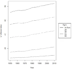
2.2 Life Expectancy of US Males, by Age, 1950–2010 . . . 13

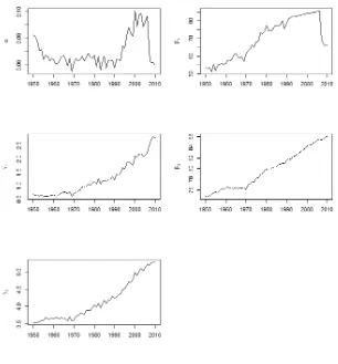
2.3 Parameter Estimates of the MCH Function for US Males . . . 14

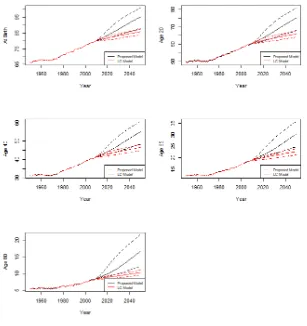
2.4 Forecasted Life Expectancy for US Males from the LC and the MCH Model with 95% Confidence Bands, by Age . . . 16

2.5 Life Expectancy of US Females, by Age, 1950–2010 . . . 19

2.6 Parameter Estimates of the MCH Function for US Females . . . 20

2.7 Life Expectancy Estimates and Forecasts with 95% Confidence Bands for the MCH Function and LC Model for US Females, by Age, 1950–2050 . . . 23

2.8 Life Expectancy of Australian Males, by Age, 1950–2010 . . . 27

2.9 Parameter Estimates of the MCH Function for Australian Males, 1950–2010 . . . . 28

2.10 Life Expectancy Estimates and Forecasts with 95% Confidence Bands for the MCH Function and LC Models for Australian Males, by Age, 1950–2050 . . . 30

2.11 Life Expectancy of Australian Females, by Age, 1950–2010 . . . 33

2.12 Parameter Estimates of the MCH Function for Australian Females, 1950–2010 . . 34

2.13 Life Expectancy Estimates and Forecasts with 95% Confidence Bands for the MCH Function and LC Models for Australian Females, by Age, 1950–2050 . . . 36

2.14 Life Expectancy of Japanese Males, by Age, 1950–2010 . . . 40

2.15 Parameter Estimates of the MCH Function for Japanese Males, 1950–2010 . . . 41

2.16 Life Expectancy Estimates and Forecasts with 95% Confidence Bands for the MCH Function and Lee-Carter Models for Japanese Males, by Age, 1950–2050 . . . 43

2.17 Life Expectancy of Japanese Females, by Age, 1950–2010 . . . 46

2.18 Parameter Estimates of the MCH Function for Japanese Females, 1950–2010 . . . 47

2.19 Life Expectancy Estimates and Forecasts with 95% Confidence Bands for the MCH Function and Lee-Carter Models for Japanese Females, by Age, 1950–2050 . . . 49

3.1 Example of the Pickands Dependence Function . . . 56

3.2 The Western North Pacific Basin (Source: http://bit.ly/2BGrDWV) . . . 59

3.3 Histogram of Wind Speed in Knots . . . 60

(12)

3.5 Scatterplot of Componentwise Maxima . . . 62

3.6 The Estimated Pickands Dependence Function by Approach . . . 62

3.7 Scatterplot of Component-Wise Maxima with 5% Storm-at-Risk Curves . . . 63

3.8 Scatterplot of Componentwise Maxima with Once-in-10-Years Storm-at-Risk Curves 64

3.9 Scatterplot of Component-Wise Maxima with Once-In-100-Years Storm-at-Risk Curves 64

4.1 Regional Map of the Philippines (Source: http://bit.ly/2mXpuTA) . . . 71

4.2 The Observed, Forecasted, and 95% FaR Values for Rice Production Volume for the

National and Macroregional Series . . . 72

CAR, Ilocos, Cagayan, and Central Luzon Regions . . . 72

CALABARZON, MIMAROPA, Bicol, and Western Visayas Regions . . . 73

Central Visayas, Eastern Visayas, Zamboanga, and Northern Mindanao Regions . 73

(13)

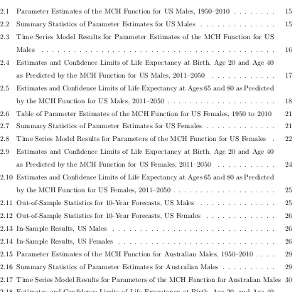
List of Tables

2.1 Parameter Estimates of the MCH Function for US Males, 1950–2010 . . . 15

2.2 Summary Statistics of Parameter Estimates for US Males . . . 15

2.3 Time Series Model Results for Parameter Estimates of the MCH Function for US Males . . . 16

2.4 Estimates and Confidence Limits of Life Expectancy at Birth, Age 20 and Age 40 as Predicted by the MCH Function for US Males, 2011–2050 . . . 17

2.5 Estimates and Confidence Limits of Life Expectancy at Ages 65 and 80 as Predicted by the MCH Function for US Males, 2011–2050 . . . 18

2.6 Table of Parameter Estimates of the MCH Function for US Females, 1950 to 2010 21 2.7 Summary Statistics of Parameter Estimates for US Females . . . 21

2.8 Time Series Model Results for Parameters of the MCH Function for US Females . 22 2.9 Estimates and Confidence Limits of Life Expectancy at Birth, Age 20 and Age 40 as Predicted by the MCH Function for US Females, 2011–2050 . . . 24

2.10 Estimates and Confidence Limits of Life Expectancy at Ages 65 and 80 as Predicted by the MCH Function for US Females, 2011–2050 . . . 25

2.11 Out-of-Sample Statistics for 10-Year Forecasts, US Males . . . 25

2.12 Out-of-Sample Statistics for 10-Year Forecasts, US Females . . . 26

2.13 In-Sample Results, US Males . . . 26

2.14 In-Sample Results, US Females . . . 26

2.15 Parameter Estimates of the MCH Function for Australian Males, 1950–2010 . . . . 29

2.16 Summary Statistics of Parameter Estimates for Australian Males . . . 29

2.17 Time Series Model Results for Parameters of the MCH Function for Australian Males 30 2.18 Estimates and Confidence Limits of Life Expectancy at Birth, Age 20, and Age 40 as Predicted by the MCH Function for Australian Males, 2011–2050 . . . 31

2.19 Estimates and Confidence Limits of Life Expectancy at Ages 65 and 80 as Predicted by the MCH Function for Australian Males, 2011–2050 . . . 32

2.20 Parameter Estimates of the MCH Function for Australian Females, 1950–2010 . . 35

2.21 Summary Statistics of Parameter Estimates for Australian Females . . . 35

[image:13.595.108.523.214.624.2]

(14)

2.23 Estimates and Confidence Limits of Life Expectancy at Birth, Age 20 and Age 40

as Predicted by the MCH Function for Australian Females, 2011–2050 . . . 37

2.24 Estimates and Confidence Limits of Life Expectancy at Ages 65 and 80 as Predicted by the MCH Function for Australian Females, 2011–2050 . . . 38

2.25 Out-of-Sample Statistics for 10-Year Forecasts, Australian Males . . . 38

2.26 Out-of-Sample Statistics for 10-Year Forecasts, Australian Females . . . 39

2.27 In-Sample Results, Australian Males . . . 39

2.28 In-Sample Results, Australian Females . . . 39

2.29 Parameter Estimates of the MCH Function for Japanese Males, 1950–2010 . . . 42

2.30 Summary Statistics of Parameter Estimates for Japanese Males . . . 42

2.31 Time Series Model Results for Parameters of the MCH Function for Japanese Males 43 2.32 Estimates and Confidence Limits of Life Expectancy at Birth, Age 20, and Age 40 as Predicted by the MCH Function for Japanese Males, 2011–2050 . . . 44

2.33 Estimates and Confidence Limits of Life Expectancy at Ages 65 and 80 as Predicted by the MCH Function for Japanese Males, 2011–2050 . . . 45

2.34 Parameter Estimates of the MCH Function for Japanese Females, 1950–2010 . . . 48

2.35 Summary Statistics of Parameter Estimates for Japanese Females . . . 48

2.36 Time Series Model Results for Parameters of the MCH Function for Japanese Females 49 2.37 Estimates and Confidence Limits of Life Expectancy at Birth, Age 20, and Age 40 as Predicted by the MCH Function for Japanese Females, 2011–2050 . . . 50

2.38 Estimates and Confidence Limits of Life Expectancy at Ages 65 and 80 as Predicted by the MCH Function for Japanese Females, 2011–2050 . . . 51

2.39 Out-of-Sample Statistics for 10-Year Forecasts, Japanese Males . . . 51

2.40 Out-of-Sample Statistics for 10-Year Forecasts, Japanese Females . . . 52

2.41 In-Sample Results, Japanese Males . . . 52

2.42 In-Sample Results, Japanese Females . . . 52

3.1 Summary Statistics for the Componentwise Maxima of Tropical Cyclones . . . 61

3.2 Confidence Intervals for χ . . . 63

(15)

Chapter 1

Introduction

Risk is present in every human activity. Our interaction with the environment and society exposes

us to dangers. These events may have miniscule probabilities of occurrence, yet their impacts can

be large, widespread and persistent. Therefore, it is vital that we gain understanding and insights

on these risks so that human activities can be managed and the impacts of these dangers can be

reduced if not eliminated.

Statistical methods pave the way to developing an understanding of risk. However, research on

the estimation and accounting of risk in various fields differs in terms of methodology. Risk in

finance has been pursued in many works of literature (Artzner et al. 1999; Jorion 2006; McNeil,

Frey & Embrechts 2005; Tsay 2005), with stylised facts over the nature of the problem cemented in

the field (Tsay 2005). Conversely, there have been open questions in pursuing risk estimation and

accounting in the fields of demography, particularly in accounting for longevity risk (Crawford, de

Haan & Runchey 2008); disasters from natural hazards (World Meteorological Organization 1999),

particularly typhoons (Okazaki, Watabe & Ishihara 2005; Yonson, Gaillard & Noy 2016); and food

security management (Jones et al. 2013; Scaramozzino 2006).

People in the Organisation for Economic Co-operation and Development (OECD) countries (OECD

2011) and in East Asia (National Institute of Ageing 2011) are living longer because of

improve-ments in health care and in access to such services. However, this exposes people to longevity risk,

defined as the exposure to dangers related to increased longevity. Although it may seem positive

at first glance, living longer is associated with practical financial considerations. For individuals,

this means the risk of a person running out of retirement benefits and savings or outliving family

or other informal sources of support (Stone & L´egar´e 2012). The risk manifests for pension fund

managers as depleted cash reserves because they are ill prepared for the increasing number of

beneficiaries and for being in contract for longer periods (Modu 2009). Government agencies that

provide benefits for their elderly citizens, such as medical care, pensions and tax breaks, are also at

(16)

In these situations, longevity risks are realised by inaccurate estimates of life expectancy and rates

of mortality (Crawford, de Haan, and Runchey 2008).

To properly account for or reduce the impact of longevity risk, there is an open field of research

in mortality modelling. This can be traced back to the Gompertz–Makeham parametric mortality

model (Gompertz 1825; Makeham 1860), which had reasonably good fit in modelling adult

mor-tality. Flexible and dynamic models of mortality for the purpose of forecasting life expectancy

have been proposed. An example of these models is the model by McNown and Rogers (1989),

which describes a parametric model for age-specific survival probability and generates forecasts

using time series analysis on the parameters. Another is by Lee and Carter (1992), which proposes

a decomposition of the central mortality rate into age-specifc and time-specific components; in

addition, forecasts of mortality rates are generated by time series analysis methods on the

time-specific component. Forecasts for life expectancy in the United States and G7 countries have been

generated using the Lee–Carter (LC) model (Tuljapurkar, Li & Boe 2000). More recently, Wong

and Tsui (2015) proposed the CH survival function, which decomposes the survival probability

into two components, the youth-to-adulthood component and the old-to-oldest component, and

fared well in fitting the US population, compared with the LC model and the Bongaarts (2005)

shifting logistic model.

In the first essay of the thesis, we propose a modified CH (MCH) survival function in which

probabilities are decomposed to the same youth-to-adulthood and old-to-oldest components, but

the number of parameters is reduced from six to five. These parameters are estimated using the

nonlinear least squares method. The parameters are then modelled using time series analysis, such

as the univariate and vector autoregressive models, and interval forecasts are generated through

residual-based bootstrapping. We show in the essay that the MCH function performs well in

long-term forecasts over the LC model for the US, Australian and Japanese populations.

Climate change has brought more intense natural hazards such as floods, cyclones, heat waves

and droughts with increasing frequency. In particular, much of temperate-climate Asia, which

covers China, the Korean peninsula, Taiwan and Japan, will experience an increase in weather

hazards, and tropical Asia, which covers much of South and Southeast Asia, is exposed to risks

of more intense cyclones, which can cause displacement of populations in low-lying areas (Mirza

2003). Thus, Southeast Asias growing economies have a higher likelihood of suffering from the

effects of climate change, compared with the rest of the world, if no policies to mitigate the risk

are established (Asian Development Bank 2009). Laos, Malaysia, Myanmar, the Philippines,

Thai-land and Vietnam are countries in the region that have cyclonic storms as their dominant disaster

risk (ASEAN Disaster Risk Management Initiative 2010), and in Japan, typhoons that occurred

from 1970 to 2004 caused the highest insurance losses in the countrys record (Okazaki, Watabe &

(17)

The intensities of typhoon characteristics were revealed as important determinants in the impacts

of cyclone disasters in the Philippines (Yonson, Gaillard & Noy 2016). Therefore, weather and

climate extremes are highlighted as major areas of concern, and estimating and predicting weather

extremes has been selected as one of the World Climate Research Programme Grand Challenges

(Sillmann et al. 2017), emphasising the importance of the problem for academics. However, even

before the posing of the challenge, modelling of extreme weather events has been conducted. There

has been extensive research on modelling extreme or maximum wind speed of hurricanes in at-risk

regions of the United States. Walshaw (2000) modelled extreme wind speeds in Boston and in the

Key West area by using the generalised extreme value (GEV) distribution (Fisher & Tippet 1928;

Gnedenko 1943) with a Bayesian approach, and concluded that standard models give misleading

results in the regions of their scope. In the Gulf Coast, Florida, and the East Coast regions of the

United States, Jagger and Elsner (2006) devised climatology models on extreme hurricane winds

by using the generalised Pareto distribution (Balkema & de Haan 1974; Pickands 1975) with both

maximum likelihood and Bayesian approaches, and generated estimates on maximum wind speed

levels for certain return periods. Wind hazard conditions on the Chinese coast were modelled

using the polynomial family of probability distributions—namely, the uniform, trapezoidal and

quadratic distributions—to generate return values for 50-year and 100-year periods (Li & Hong

2015). Annual maximum wind conditions in the western North Pacific region were estimated using

the Gumbel distribution, a special case of the GEV distribution, and there was fair agreement

between the estimated and observed 48-year wind maxima for the extreme winds data from the

Philippines (Ott 2006). Estimations of extreme wind and pressure events for storms were conducted

by Economou, Stephenson and Ferro (2014) for the northern Atlantic basin by using point process

extreme value models with the North Atlantic Oscillation index (NAO) as a significant covariate in

the model, and a negative relationship was revealed between minimum pressure levels and the NAO.

The second essay of the thesis proposes an estimation procedure for the threshold estimation

of extreme wind and pressure characteristics, similar in concept to the value-at-risk (Jorion 2006),

which we call the storm-at-risk. The proposed risk measure is estimated using the multivariate

extreme value distribution (Pickands 1981) with bootstrapped confidence interval forecasts. We

demonstrate the methodology on typhoon data for the western North Pacific basin, which includes

the high-at-risk regions of East and Southeast Asia. For lower coverage probabilities and lower

return periods, the nonparametric storm-at-risk curves provide more robust results within desired

coverage probabilities. For higher coverage probabilities, the semiparametric approach provides

more robust results within the desired coverage.

Food security, as defined by the World Food Summit (1996, p. 4, par. 1, clause 2), ’exists

when all people, at all times, have physical and economic access to sufficient, safe and nutritious

(18)

defini-tion underlines four key dimensions of food security: availability; access; utilisadefini-tion; and stability

(Food and Agricultural Organization 2016). The key contributing factors to food security in

de-veloping countries are agricultural productivity, foreign exchange earnings and population growth.

By increasing production, increasing food imports and reducing population growth, developing

countries can achieve food security (Shapouri & Rosen 1999). If left unchecked, food insecurities

and emergencies threaten long-term development in developing countries and increase the risk

of communities of these countries to future disasters (Haile & Bydekerke 2012). By developing

risk assessment and analysis systems, risk mapping, and monitoring and early warning systems,

governments in developing countries can manage and reduce the impact of food insecurity (Asian

Development Bank 2013; Haile & Bydekerke 2012).

Measuring food security risk is an open research question. A compendium of food security metrics

has been provided by Jones et al. (2013). They described the metrics by their purposes—namely,

(1) to provide national estimates of food supply, (2) to inform global monitoring and early warning

systems, (3) to assess household food access and acquisition and (4) to measure food consumption

and utilisation. Scaramozzino (2006) proposed a value-at-risk approach to measuring vulnerability

to food security. The methodology introduced a financial risk management style to mitigating

and addressing food security risk, considered of particular importance in the area of early warning

systems (Haile & Bydekerke 2012).

With the ideas of using value-at-risk methodologies in food insecurity, providing a measurement to

be used for early warning systems, and an estimation system that can provide national and

sub-national estimates, we propose a food security risk estimation method called food-at-risk in the

third essay. It adapts the forecast reconciliation methodology of Hyndman et al. (2011) and

Hyn-dman, Lee and Wang (2016) to produce consistent and agreeable time series forecasts for national

and sub-national estimates. The reconciliation method is bootstrapped to produce the desired risk

measure for a defined probability of risk. We apply the estimation technique on Philippine regional

rice production data.

1.1 Significance

The significance of the proposed methodologies is in their uses in providing information and

under-standing of the risks that each methodology addresses. In proposing the MCH function, adequately

forecasted life expectancy can make pension fund institutions more solvent by having adequate cash

reserves to continue servicing clients (Modu 2009). Robust life expectancy forecasts in the long

term can also help government agencies that serve the elderly to manage their resources (Stone &

L´egar´e 2012) and properly estimate cash inflows and outflows of the services. These concerns can

(19)

For disaster risks from extreme weather events, the understanding and prediction of these events

has been posed as a global challenge to all researchers in the field (Sillmann et al. 2017). Proper

estimation of extreme weather conditions is also vital for insurance companies that give financial

support in cases of disasters due to such natural hazards (Okazaki, Watabe & Ishihara 2005).

Estimates from the proposed methodology in the second essay can guide disaster risk managers

and policymakers for appropriate plans of action in case of severe cyclonic storms.

Measuring food security risks is vital to facilitate growth in developing countries and combat

extreme poverty (Asian Development Bank 2013; Food and Agricultural Organization 2016; Haile

& Bydekerke 2012). Estimation of food security risk requires a multi-level approach that provides

understanding on national and local levels. The food-at-risk information system proposed by the

third essay addresses the concerns of food insecurity by examining the level of food supply at both

national and sub-national levels.

1.2 Outline

The thesis is assembled as follows. Chapter 1 covers the introduction to the theme of the thesis

and a discussion of the significance of the proposed methods. Longevity risk is addressed by

the proposed survival model called the MCH function in the first essay presented in the second

chapter. The second essay discusses the storm-at-risk curves methodology and is presented in the

third chapter. A discussion of the food-at-risk methodology is presented in the fourth chapter of

the thesis. Finally, the fifth chapter contains the conclusion and summary of the thesis with a

(20)

Chapter 2

Longevity Risk: Forecasting Life

Expectancy

2.1 Introduction

Improvements in healthcare services and increased access to these services over the past 50 years

have resulted in populations living longer than previously anticipated. The United Nations

Depart-ment of Economic and Social Affairs, Population Division (2012) reported that a growing number

of populations around the world have had positive trends in their life expectancies at birth, from

an average of approximately 48 years of age in 1950–1955 to 68 years in 2005–2010. For member

countries in the OECD, life expectancy at birth in 2008 was 79.3 years, with an average

differ-ence of life expectancy over all OECD countries of 6 years from 1983 to 2008 (OECD 2011). Such

trends reflect the general improvement in the quality of life in the world with lower mortality rates.

With growing elderly populations, an increase in costs and demand for aged healthcare,

retire-ment plans, and pensions provided by financial institutions is observed or can be anticipated,

along with increased utilization of government healthcare services for senior citizens. A rough

es-timate on a five-year improvement on longevity for retirement-age individuals in the United States

would mean an increase on the present value of benefits by 10% to 15%. Insurance portfolios with

many old individuals and few active employees that contribute to revenues are heavily affected

by changes in mortality (Gutterman, et al 2002). Demand for full-time physicians in the United

States is expected to rise from 778,200 physicians in 2013 to between 865,000 to 911,400

physi-cians in 2025 that should be fulfilled by the government and private sectors (IHS Inc. 2015). An

increase of 50% in the proportion of Americans that will receive healthcare through the Medicare

program between 2000 and 2050 is expected. The cost of Medicare expected to increase from 2.2%

of GDP in 2000 to 6% of GDP in 2050. Total cost of all available services for the elderly, which

includes Medicare, Social Security, and Medicaid long-term care is expected to increase from 6.8%

(21)

United States may increase from 5% of the non-elderly adult population in 2010 to a low scenario

of 7% or a high scenario of 11% in 2050. (Congressional Budget Office 2013). As these examples

demonstrate, it is imperative for these institutions to assess and prepare for the risks associated

with increased cash outflows due to the growing elderly population.

One type of risk associated with the growing elderly population is known as longevity risk, which

arises because of unexpectedly high life expectancies leading to higher payout and other cost ratios

for private financial institutions (Modu 2009) and government agencies (Stone & L´egar´e 2012).

An example of impending longevity risk to governments is the report of the Board of Trustees,

Federal Old-Age and Survivors Insurance and Federal Disability Insurance Trust Funds (2015) of

the United States, which states that the balances among their income rates, excluding interest

income and cost rates, have been in the negative range since 2009, and may continue to be in the

negative up to the year 2090, in the three scenarios of low-, intermediate- and high-cost situations.

The negative balance is due to the baby-boom generation moving to the retirement and senior

cohort in 2016–2035 and the declining death rates forecast in 2050–2089. To address such risk,

institutions initially prepare models to forecast future mortality tables and to design policies or risk

transfer products. These models enable them to not only create improved products and services in

response to growing demand from the elderly population but also reduce their exposure through

the process of reinsurance. Therefore, the development of accurate mortality forecasting models is

vital for these institutions.

Given these concerns, current mortality models have shortcomings in terms of forecasting accuracy.

Before 1992, mortality forecasting was constructed through structural econometric modelling of

socioeconomic and demographic factors (e.g., Land 1986; Olshansky 1988) or deterministic

cohort-component forecasts (e.g., Alho 1990; Guralnik, Yanagishita & Schneider 1988). However, these

methodologies produced unsatisfactory forecasts for longevity (Giacometti et al. 2012) until the

methodology of Lee and Carter (1992), using a statistical time series forecasting approach, was

in-troduced into a demographical model of mortality. This model, however, had flaws documented in

the literature. Its strict assumptions on age-specific components have been empirically disproven,

and the model was extended for this criterion (Li, Lee & Gerland 2013). The model has performed

very well in forecasting life expectancies for lower and middle starting ages but has been found

poor for older ages, where longevity risk is more imminent (Wong & Tsui 2015). Leng and Peng

(2016) concluded that the LC model and its extensions in the literature cannot describe the true

dynamics of the mortality index, which may lead to questionable forecasts and projections on

mor-tality. With these considerations, we propose a model that addresses these issues with improved

forecasting ability.

By synthesising the existing statistical methodologies of forecasting mortality, we show that our

(22)

first step is the estimation of a survival function from mortality tables within each year. The

sur-vival function, the MCH function, is based on a simplified form of the Wong and Tsui (2015) CH

function, which considers two components of survivability: young-to-old and old-to-oldest

compo-nents. Changing trends in the oldest cohort, which are different from those in the younger cohorts,

is the consideration of the CH function. The MCH function has a reduced number of parameters

and pragmatic parameter constraints, which improves longevity estimates and the interpretability

of the function parameters. A mix of univariate and multivariate time series analysis through

autoregressive models is performed to generate longevity forecasts. Autoregressive models take

into account the autocorrelation of each MCH parameter, and the vector form of the model the

cross-correlation between parameters within each MCH component, which improves forecasting

ability by reducing estimation errors. To augment longevity forecasts, residual-based multivariate

bootstrapping is used in generating confidence intervals. To demonstrate the methodology, the

US, Australian and Japanese male and female life tables from 1950 to 2010 were used. Results on

confidence intervals and forecasted life expectancies are shown. Robustness checks through

cross-validation forecast error statistics and the Diebold–Mariano (DM) test (Diebold & Mariano 1995)

for forecasting comparisons with the LC model are shown below. We have concluded that the

proposed procedure performs favourably over the LC model in terms of out-of-sample forecasting.

The remainder of the chapter is constructed as follows. The second part describes the

mathe-matical background of the LC and Wong–Tsui models. Our proposed methodology is discussed

in detail in the third part. A discussion on the steps of demonstrating the method with the US,

Australian and Japanese annual life tables is outlined in the fourth part, with discussion of the

results in the fifth part. We provide our conclusions on the methodology in the sixth part of the

chapter.

2.2 Background Literature

Lee and Carter (1992) proposed a methodology for modelling mortality rates and forecasting life

expectancy by using the following decomposition model; denoting mx,t as the matrix of central

mortality rates, it is assumed that:

log (mx,t) =ax+bxkt+x,t (2.1)

where ax is the main component of age in mortality, bx is the interaction factor of age to and

independent of time, and kt is defined as the mortality index of time. They are estimated by

singular value decomposition, andktis reestimated to conform with the relationship:

(23)

where D(t) is the observed number of deaths in timet, andN(x, t) is the population distribution for age x in a given time t. To make forecasts, it is assumed that ax and bx will not change in time and ktis fitted with an econometric model. According to Lee and Carter (1992), the model

is estimated with a random walk with drift and an exogenous variable, flu, which accounts for the

1918 influenza outbreak:

kt=kt−1−0.365 + 5.24flu +et (2.3)

From the econometric model ofktand the structural model of log (mx,t), forecasted life tables and

life expectancies are generated.

However, the original LC model is too restrictive in its assumptions, such asbxbeing constant in

time (Li, Lee & Gerland 2013), and is not suitable for inference (Leng & Peng 2016); thus, it has

not performed well in forecasting for older ages over time (Wong & Tsui 2015), which warrants

alternative models for forecasting longevity.

Wong and Tsui (2015) proposed a methodology for forecasting life expectancy by using a new

survival function and combining the function with autoregressive models to facilitate forecasting.

The CH survival functionSCH(x) of Wong and Tsui (2015) is specified as follows:

SCH(x) =α1exp{−exp{(x/β1)γ1}}+α2exp{−cosh{(x/β2)γ2}} (2.4)

whereα1andα2act as weights,β1andβ2act as scaling parameters and give information on typical

ages that distinguish each component, andγ1andγ2describe the shape of the two components on

how fast the survival probabilities descend to zero as the age xincreases. The parameter ranges are as follows: α1, α2, β1, β2, γ1, γ2>0. The first addend corresponds to the ”youth-to-adulthood”

component whilst the second is the ”old-to-oldest-old” component.

In the methodology by Wong and Tsui (2015) for each life table in yeart= 1,2, . . . , T, the param-eters are estimated by nonlinear least squares, creating the parameter series {α1,t}Tt=1,{β1,t}Tt=1,

{γ1,t}Tt=1, {α2,t}Tt=1,{β2,t}Tt=1, and {γ2,t}Tt=1. Each parameter series is modeled individually by

rate of change differencing and univariate autoregressive models (Box, Jenkins & Reinsel 1994),

such as the AR(1) model as shown below:

∆yt

yt

=µ+φ1

_∆_y

t−1

yt−1

−µ

+t, t∼ 0, σ2

(2.5)

From the estimtes of the model above, forecasts on parameter values are generated and life

ex-pectancy estimates ˜ex at age x are generated by actuarial methods, in which for any survival functionS(x):

˜

ex= ∞

X

kpx+ 1

2, kpx=

S(x+k)

(24)

Based on the results from in-sample and out-of-sample forecasts, the Wong and Tsui (2015)

method-ology outperforms that of Lee and Carter (1992).

2.3 Proposed Methodology

We notice certain parameter relationships and structures in the Wong and Tsui (2015) model

whereby the model can be further simplified to enhance the estimation process. They are:

α1+α2=e, α1≤α2, β1≤β2, γ1≤γ2 (2.7)

When evaluated at zero, SCH(0) = (α1+α2)e−1. To force the value to 1, α1e−1 = α and

α2e−1= 1−α, thus making equation (2.8) below. In the paper of Wong and Tsui (2015),α1≤α2

for any year, emphasising that survivability is domimated by the old-to-oldest-old component over

the youth-to-adulthood component. For the new parameter, α ≤ 1−α, thus α ≤ 0.5. The relationships for β1, β2, γ1 andγ2 are based on the features of the components in the original CH

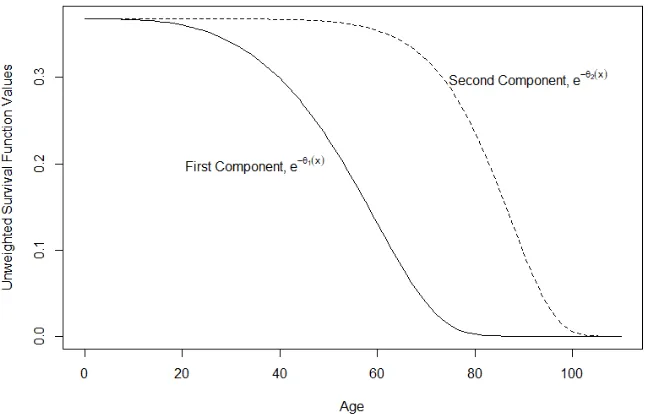
[image:24.595.136.460.417.624.2]

function results. The relationship is shown in Figure 2.1.

Figure 2.1: Unweighted CH Components Using Wong and Tsui’s (2015) Results for US Females for the Year 2000

The parameter β1 is related to the centre of the first component, and β2 the second. As the first

is linked to youth-to-adulthood, compared with old-to-oldest-old for the second, the centre of the

first is less than or equal to the centre of the second; thus, β1 ≤β2. The parameters γ1 and γ2

are polynomial powers with respect to the speed of reaching zero survival probability. With links

to age periods of an individuals life, the speed of the first is less than or equal to the speed of the

(25)

We propose the MCH survival function, which has a reduced number of parameters and

main-tains appropriate properties as a survival function:

SM CH(x) =αexp{−exp{(x/β1)γ1}+ 1}+ (1−α) exp{−cosh{(x/β2)γ2}+ 1}. (2.8)

The MCH survival function has the following parameter space:

α≤0.50,0< β1≤β2,0< γ1≤γ2 (2.9)

To create life expectancy forecasts, let lx(t) be the number of lives age xat year t = 1,2, . . . , T. The parameters {αt}Tt=1,{β1,t}Tt=1, {γ1,t}Tt=1,{β2,t}Tt=1,{γ2,t}Tt=1 are estimated by minimising the

sum of square errors (SSE) for all yearst, where xmax is the maximum age:

SSE(t) = xmax

X

x=0

[lx(t)−100,000SM CH,t(x)]

2

(2.10)

A pα-order autoregressive [AR(pα)] model is fitted to the adjusted parameter series {f1(αt)}Tt=1,

while api-order vector AR [VAR(pi)] model (L¨utkepohl 2006; Sims 1980) is fitted on the adjusted parameter vector series{θt(1)}Tt=1 ={[f2(β1,t), f3(γ1,t)]

0

}T

t=1and{θ (2)

t }Tt=1={[f4(β2,t), f5(γ2,t)] 0

}T t=1

:

θ(_ti)= pi

X

j=1

Φ(_ji)θ_t(i₋)_j+(_ti); (_ti)∼0,Σ(i), i= 1,2 (2.11)

A life table is generated on the basis of SM CH(x) by using the in-sample predictions {µt}Tt=1 =

{µα

t, µ

(1)

t

0

, µ(_t2)0}T

t=1and k-periods forecasts{µt}tT=+Tk+1 of the AR(pα) and VAR(pi) models for the parameters with their formulas shown below:

µα_t = pα

X

i=1

ˆ

Φα_if1(αt−i) ;µ(ti)= pi

X

j=1

ˆ

Φ(_ji)θ(_t−ji) , i= 1,2 (2.12)

The life expectancy{˜ex,t}Tt=1+k for agexat yeart is derived from the estimated life table by using

equation (2.6).

The blocked AR(1)–VAR(1) modeling approach was chosen to make forecasts of MCH

param-eter values. One may use higher orders for forecasting, but because of the paramparam-eters estimation

on each year would produce short time series data, e.g., for the real data application, there would

be 60 annual periods of data, higher orders would risk convergence issues, especially on

bootstrap-ping later.

Residual-based bootstrapping (Paparoditis & Streitberg 1991) can be used to generate confidence

(26)

• From the AR(pα) and VAR(pi) models in equations (2.5), (2.11) and (2.12), the residual vectors{ˆt}Tt=1 where ˆt=θt−µt are generated.

• LettingnB be the number of bootstrap samples to be generated, the bootstrapping is looped forb= 1,2, . . . , nB

1. a bootstrap sample of residual vectors {et,b}Tt=1 is drawn from {ˆt}Tt=1 and get θ˜t,b =

µt+et,b.

2. AR(pα) and VAR(pi) models are fitted to{θ˜t,b}Tt=1.

3. A life table is generated based onSM CH(x) by using the in-sample predictions{µ˜t,b}Tt=1

and k-periods forecasts{µ˜t,b}tT=+Tk+1 ofAR(pα) and VAR(pi) models for the parameters:

µα_t,b= pα

X

i=1

ˆ

Φα_i,bf1(αt−i) ;µ

(i)

t,b = pi

X

j=1

ˆ

Φ(_j,bi)θ(_t−ji) , i= 1,2 (2.13)

4. The life expectancy ˜ex,t,bis estimated from the generated life table using equation (2.6).

• The (1−α) 100% confidence interval for ex,t for age x at time t, with ˜ex,t,(k) meaning the

kth smallest value of ˜ex,t,b, is:

˜

e_x,t,_([_n

Bα2])

,˜e_x,t,_([_n

B2−2α])

(2.14)

We adjust the parameters using the following functions:

f1(rt) = log

rt 1−rt

−log

rt−1

1−rt−1

(2.15)

fq(rt) = log (rt)−log (rt−1), q= 2,3,4,5 (2.16)

where the first function is called the dlogit function while the second function is called the dlog

function.

2.4 Methodology Demonstration

The MCH methodology is demonstrated on the US, Australian and Japanese annual life tables

data for males and females in 1950–2010. The data were downloaded on 2 January 2016 from the

Human Mortality Database. Life expectancy is evaluated at ages 0 (at birth), 20, 40, 65 and 80,

and forecast for 2011–2050, with 95% confidence intervals. The predictive performance of the MCH

model is compared with that of the LC model, as set up in the demography package (Hyndman et

al. 2014) in R and performed with 10 years of hold-out data (2001–2010). The in-sample period

(27)

comparisons are the mean absolute error (MAE) and the two-sided one-step-ahead DM test:

M AE= 1

n

X

i=1

|actuali−predictedi| (2.17)

DM = ¯

d

q

ˆ

σ2

d

n

∼N(0,1) as n→ ∞ (2.18)

di= error2i,model1

− error2_i,model₂, i= 1,2, . . . , n

¯

d= 1

n

X

i=1

di; σˆ2d= 1

n

X

i=1

di−d¯

2

2.5 Discussion of Results

2.5.1 US Life Tables

The following graphs show the descriptive statistics and table of results of the demonstrations on

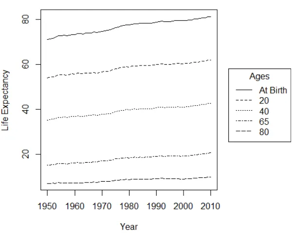
US data. From Figure 2.2, the graph of life expectancy values for US males in 1950–2010, there is

an upward trend in life expectancy over all ages. The trend, however, becomes flatter as we solve

for the life expectancy from birth up to age 80.

(28)

Figure 2.3: Parameter Estimates of the MCH Function for US Males

Figure 2.3 is the graph of the parameter estimates of the proposed methodology over the covered

period. From the estimated parameter series of the MCH function for US males, the beta and

gamma parameters generally have an upward trend starting at 1960 for the first component, while

it starts at 1970 for the second component. The alpha parameter for males is relatively flat from

1950 to the mid-1980s before developing an increasing trend. For the parameters of the

youth-to-adulthood component and alpha, there is a decline in 1995–1998. After the period, the parameters

show an upward trend. The upward trend in alpha signifies that, for the MCH function, the

survivability of US males tends to have bigger weight on the youth-to-adulthood component than

the old-to-oldest component. The numerical results can be found in Table 2.1. It shows the

R-square of the fit of the proposed survival function for each life table of the years. The R-R-square is

(29)

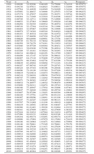
Table 2.1: Parameter Estimates of the MCH Function for US Males, 1950–2010

Year α β1 γ1 β2 γ2 R-square

1950 0.08095 30.11515 0.40597 68.41750 2.65831 99.9913% 1951 0.08103 29.93896 0.40632 68.42830 2.65243 99.9913% 1952 0.08068 30.34482 0.40610 68.52568 2.64008 99.9918% 1953 0.07751 30.34034 0.40948 68.63079 2.66238 99.9924% 1954 0.07346 31.22199 0.40086 69.20069 2.68720 99.9938% 1955 0.07389 32.74988 0.41938 69.21561 2.72225 99.9935% 1956 0.07239 32.39476 0.41693 69.17866 2.72373 99.9934% 1957 0.07048 30.48612 0.40228 68.84197 2.70013 99.9938% 1958 0.06931 30.49449 0.39826 69.05374 2.72126 99.9941% 1959 0.06885 30.71491 0.40347 69.17052 2.71678 99.9942% 1960 0.06737 30.50508 0.39402 68.95348 2.71379 99.9946% 1961 0.06557 30.97055 0.40319 69.27922 2.72768 99.9943% 1962 0.06551 31.30714 0.41157 69.11689 2.73227 99.9942% 1963 0.06638 32.00199 0.41426 68.88007 2.73504 99.9942% 1964 0.06802 34.17906 0.43169 69.07630 2.71714 99.9940% 1965 0.06778 35.03456 0.44516 69.02151 2.72528 99.9939% 1966 0.06907 36.80348 0.46590 68.90725 2.71691 99.9938% 1967 0.07036 39.43931 0.49888 69.13815 2.72655 99.9937% 1968 0.07355 41.67378 0.52163 68.82065 2.72551 99.9933% 1969 0.07724 44.53032 0.56013 69.10719 2.73634 99.9930% 1970 0.07511 45.44515 0.55294 69.22324 2.72842 99.9934% 1971 0.07576 47.54643 0.60456 69.55554 2.76717 99.9937% 1972 0.07599 50.30757 0.62171 69.50683 2.78079 99.9940% 1973 0.07791 50.74621 0.65488 69.78869 2.80689 99.9940% 1974 0.07446 50.95305 0.65381 70.24518 2.82478 99.9944% 1975 0.07446 53.86511 0.67012 70.68670 2.84371 99.9944% 1976 0.06924 52.10698 0.67292 70.92032 2.86460 99.9952% 1977 0.07268 55.17276 0.70741 71.29319 2.88723 99.9952% 1978 0.07249 55.34002 0.73464 71.50546 2.90888 99.9953% 1979 0.07577 57.59404 0.77553 71.95174 2.93341 99.9953% 1980 0.07737 57.69412 0.81587 71.99930 2.97635 99.9954% 1981 0.07583 59.83110 0.83509 72.28147 2.98844 99.9958% 1982 0.07182 61.14238 0.80319 72.52052 3.01096 99.9960% 1983 0.06912 61.25181 0.80906 72.59878 3.04672 99.9963% 1984 0.07057 61.13745 0.85033 72.80760 3.05938 99.9964% 1985 0.07439 61.39307 0.89244 72.89652 3.08677 99.9961% 1986 0.08551 64.34461 0.98015 73.22052 3.12722 99.9958% 1987 0.08748 64.89376 1.01540 73.42686 3.14253 99.9957% 1988 0.09290 64.38272 1.08298 73.63627 3.18058 99.9955% 1989 0.09767 65.74466 1.12399 74.00277 3.18590 99.9952% 1990 0.10221 66.94121 1.16918 74.33765 3.21839 99.9954% 1991 0.10672 67.67891 1.22399 74.61203 3.24841 99.9955% 1992 0.11049 68.05616 1.31155 74.97004 3.27886 99.9956% 1993 0.11890 68.49314 1.37511 75.02808 3.33222 99.9954% 1994 0.12531 68.89534 1.45257 75.39440 3.36609 99.9952% 1995 0.12990 69.59608 1.52239 75.65471 3.41353 99.9955% 1996 0.11206 68.55962 1.46137 75.74452 3.41415 99.9956% 1997 0.09784 67.11171 1.40237 75.93831 3.43579 99.9956% 1998 0.09587 67.52334 1.41170 76.14474 3.46258 99.9955% 1999 0.10167 68.26278 1.50436 76.38578 3.52459 99.9949% 2000 0.10924 68.74757 1.59542 76.77923 3.57414 99.9944% 2001 0.11877 69.62737 1.67230 77.14243 3.61613 99.9943% 2002 0.12659 69.73075 1.75944 77.45423 3.66942 99.9929% 2003 0.13273 70.28062 1.81182 77.78716 3.69407 99.9920% 2004 0.13812 71.11015 1.86885 78.35483 3.73799 99.9913% 2005 0.14560 71.23329 1.91736 78.57172 3.77952 99.9903% 2006 0.15237 71.93645 1.95606 79.02906 3.81209 99.9903% 2007 0.15220 72.22768 1.97260 79.30786 3.82040 99.9895% 2008 0.15089 72.33843 2.01870 79.37364 3.82377 99.9893% 2009 0.15795 73.10333 2.12437 79.85772 3.84719 99.9891% 2010 0.15314 73.28042 2.13050 79.95006 3.85749 99.9899%

Table 2.2: Summary Statistics of Parameter Estimates for US Males

α β1 γ1 β2 γ2

(30)

Table 2.3: Time Series Model Results for Parameter Estimates of the MCH Function for US Males

Terms Equations

dlogit(α) dlog(β1) dlog(γ1) dlog(β2) dlog(γ2)

constant 0 0.011175* 0.019413*** 0.0019562*** 0.003796*** (se) - - 0.004336 0.005389 0.0005534 0.001084 dlogit(α).l1 0.4948***

(se) 0.1106

dlog(β1).l1 0.205536 0.014588

(se) 0.148681 0.18478 dlog(γ1).l1 0.032339 0.301317*

(se) 0.117308 0.14579

dlog(β2).l1 -0.0916912 0.601523*

(se) 0.148069 0.29011

dlog(γ2).l1 0.1471083* 0.155718

(se) 0.0713006 0.139699 Signifincance codes: 0 *** 0.001 ** 0.01 * 0.05 . 0.1 1

se: standard error; l1: lag of order 1

Table 2.3 above shows the results of the time series models used in estimating the in-sample

predictions for the data from 1950 to 2010 and forecasts from 2011 to 2050.

Figure 2.4: Forecasted Life Expectancy for US Males from the LC and the MCH Model with 95% Confidence Bands, by Age

Figure 2.4 shows graphs of estimates and forecasting results by the proposed methodology and the

(31)

MCH model indicated in black lines. The proposed methodology tends to have higher forecasted

values, compared with the LC model, over all ages. We show the confidence interval estimates

from the MCH model in Tables 2.4 and 2.5 .

Table 2.4: Estimates and Confidence Limits of Life Expectancy at Birth, Age 20 and Age 40 as Predicted by the MCH Function for US Males, 2011–2050

˜

e0 e˜20 e˜40

(32)

Table 2.5: Estimates and Confidence Limits of Life Expectancy at Ages 65 and 80 as Predicted by the MCH Function for US Males, 2011–2050

˜

e65 ˜e80

(33)

[image:33.595.161.464.135.378.2]

Figure 2.5: Life Expectancy of US Females, by Age, 1950–2010

Figure 2.5 shows the life expectancy values for US females from 1950 to 2011 based on the life

table data. For life expectancies at birth, age 20 and age 40, there are greater increases from 1950

(34)

Figure 2.6: Parameter Estimates of the MCH Function for US Females

Figure 2.6 is a graph of the parameter estimates for US females for the coverage period. In

contrast to US males, US females do not show a decline; each series has an upward trend. The

alpha parameter is relatively flat from 1950 to 1990, before having a positive trend from the latter

year. This may mean that the youth-to-adulthood component became more important for the

survivability of US females by 1990. We show the parameter results in Table 2.6 and the summary

(35)

Table 2.6: Table of Parameter Estimates of the MCH Function for US Females, 1950 to 2010

Year α β1 γ1 β2 γ2 R-square

1950 0.08189 48.67920 0.55321 74.15176 3.22102 99.9784% 1951 0.08043 48.27816 0.54550 74.31886 3.23815 99.9771% 1952 0.07920 47.88114 0.53399 74.58214 3.24694 99.9789% 1953 0.07440 48.25102 0.53128 74.77087 3.27897 99.9799% 1954 0.07050 49.17792 0.52630 75.36778 3.30127 99.9815% 1955 0.07104 50.76786 0.55049 75.48524 3.37506 99.9811% 1956 0.07032 51.29027 0.55830 75.58754 3.38602 99.9810% 1957 0.07150 50.29155 0.57071 75.45447 3.37633 99.9804% 1958 0.07010 50.22395 0.55866 75.68344 3.41271 99.9798% 1959 0.07051 51.65296 0.58318 75.98405 3.44124 99.9797% 1960 0.07092 52.06526 0.61022 75.98184 3.44122 99.9786% 1961 0.07160 54.38907 0.63590 76.34274 3.47330 99.9775% 1962 0.07407 55.62843 0.67478 76.29007 3.49355 99.9758% 1963 0.07514 55.51552 0.69395 76.24484 3.49379 99.9747% 1964 0.07681 56.72273 0.71750 76.58941 3.49125 99.9733% 1965 0.07832 58.33628 0.75540 76.70482 3.50982 99.9726% 1966 0.07892 58.98006 0.77627 76.73143 3.51960 99.9741% 1967 0.07979 60.66701 0.82167 77.04581 3.52761 99.9742% 1968 0.08181 60.83825 0.86049 76.84493 3.52367 99.9736% 1969 0.08367 62.10180 0.88411 77.18176 3.54742 99.9748% 1970 0.07995 62.07443 0.86107 77.26970 3.48598 99.9771% 1971 0.08418 64.32276 0.97047 77.62210 3.55474 99.9772% 1972 0.08128 64.88285 0.98108 77.60740 3.54972 99.9808% 1973 0.08500 65.92812 1.05277 77.90969 3.60356 99.9783% 1974 0.08225 66.72579 1.06072 78.32620 3.62504 99.9789% 1975 0.07802 67.43809 1.03327 78.75834 3.60050 99.9807% 1976 0.08022 67.95235 1.12829 79.02873 3.66349 99.9791% 1977 0.07967 68.97214 1.15175 79.34762 3.64862 99.9808% 1978 0.08058 69.33938 1.19652 79.50536 3.68089 99.9808% 1979 0.07801 70.47728 1.17953 79.81389 3.68825 99.9820% 1980 0.07629 69.64567 1.19702 79.58017 3.69560 99.9827% 1981 0.07746 71.00797 1.26510 79.85069 3.69934 99.9825% 1982 0.06809 70.31424 1.15823 79.86322 3.65226 99.9852% 1983 0.06890 70.05545 1.23786 79.87698 3.68262 99.9846% 1984 0.06753 69.81607 1.23159 79.92710 3.67813 99.9856% 1985 0.06943 70.17602 1.29379 79.96550 3.71042 99.9851% 1986 0.06814 69.80634 1.27893 80.02796 3.69927 99.9867% 1987 0.07136 70.27538 1.34449 80.20092 3.73185 99.9860% 1988 0.07433 70.81702 1.37676 80.23119 3.76949 99.9853% 1989 0.07032 70.10697 1.30555 80.41992 3.74591 99.9866% 1990 0.07304 71.70889 1.40884 80.67979 3.76176 99.9870% 1991 0.07603 72.28957 1.48708 80.85339 3.78368 99.9873% 1992 0.07463 72.91817 1.49993 80.98068 3.77934 99.9886% 1993 0.08035 73.13215 1.58260 80.88050 3.84321 99.9884% 1994 0.08471 74.51214 1.63834 81.04775 3.87435 99.9892% 1995 0.09031 75.15524 1.74627 81.16258 3.92104 99.9893% 1996 0.08868 75.69606 1.75452 81.22504 3.94099 99.9899% 1997 0.08997 75.94906 1.81942 81.39663 3.98712 99.9895% 1998 0.08793 76.24137 1.79068 81.39981 4.01005 99.9898% 1999 0.09600 76.93670 1.92223 81.46115 4.09125 99.9898% 2000 0.10182 77.60422 2.00722 81.62740 4.13560 99.9900% 2001 0.11662 79.47767 2.12930 81.91480 4.21593 99.9902% 2002 0.12188 79.73437 2.17725 82.10375 4.27344 99.9901% 2003 0.13119 80.06556 2.28186 82.40594 4.33596 99.9895% 2004 0.13298 81.20804 2.26849 82.76715 4.34646 99.9894% 2005 0.14382 81.70747 2.36454 82.96676 4.43979 99.9892% 2006 0.14809 82.20330 2.38924 83.32211 4.46455 99.9891% 2007 0.14525 82.37390 2.36431 83.53216 4.47097 99.9892% 2008 0.14927 82.29292 2.46103 83.61380 4.50819 99.9896% 2009 0.15870 83.99502 2.48258 83.99502 4.50301 99.9906% 2010 0.15678 84.10306 2.52350 84.10310 4.53919 99.9913%

Table 2.7: Summary Statistics of Parameter Estimates for US Females

α β1 γ1 β2 γ2

Mean 0.08820 66.90455 1.28436 79.11337 3.74902 Maximum 0.15870 84.10306 2.52350 84.10310 4.53919 Minimum 0.06753 47.88114 0.52630 74.15176 3.22102 Standard Deviation 0.02491 10.85392 0.61419 2.75112 0.35749 Skewness 1.76578 -0.31109 0.57652 -0.05410 0.83534 Excess Kurtosis 1.88193 -1.01046 -0.78920 -1.06648 -0.16928

Comparing the differences between the sexes for the US population from tables 2.1and 2.6, the

females tend to have higher values inβ1,γ1,β2, andγ2. Theβ parameters are associated with the

(36)

having higher values in theβ parameters, this implies that females typically live longer than males, which agrees with typically observed life expectancy values as seen in Figures 2.2 and 2.5.

The γ parameters for females are always higher than the males. These are attributed to the speed in which zero survival probability is reached for each of the two components of the MCH

function. Higherγ values mean that once the typical age of has been achieved by the individual, the probability of surviving more years declines faster than having lower γ values. For the dif-ference between the sexes in the US, this means that once females reach the typical age of their

component in which they belong as described by the β parameter, their chance of survival will decline faster than when males in the same situation with respect to their typical age.

With the α parameters between the sexes, the US males had an incline between 1984 to 1995, but dropped from 1996 to 1998 to be in the same levels as the female population. As this

parame-ter is inparame-terpreted as the contribution of the youth-to-adulthood component to overall longevity, this

meant that from the period of 1984 to 1995, the youth-to-adulthood related activities grew more

important for the longevity of males. This may be attributed to the changing demographic for US

males in the period. The years 1996 to 1998 were an adjustment period for the US male population

to be in line with females with respect to the importance of youth-to-adulthood component. From

1998 onwards, the patterns between males and females in terms of theαparameters were similar which meant that from the start of the new millennium, the importance of the components in

terms of survivability have become similar between the sexes.

Table 2.8 shows the results of time series model estimation used to generate the estimates and

forecasts of the life expectancy for US females in the prescribed periods.

Table 2.8: Time Series Model Results for Parameters of the MCH Function for US Females

Terms Equations

dlogit(alpha) dlog(beta1) dlog(gamma1) dlog(beta2) dlog(gamma2) constant 0.0121* 0.00938*** 0.030895*** 0.0022543*** 0.006617*** (se) 0.0069 0.002115 0.005802 0.0004257 0.001597 dlogit(alpha).l1 0.1163

(se) 0.1279

dlog(beta1).l1 -0.011813 0.613764 (se) 0.150873 0.413896 dlog(gamma1).l1 0.005402 -0.416918** (se) 0.051363 0.140906

dlog(beta2).l1 -0.1242139 0.106631

(se) 0.1338445 0.502054

dlog(gamma2).l1 0.0183699 -0.196858

(se) 0.0352951 0.132393

Significance codes: 0 *** 0.001 ** 0.01 * 0.05 . 0.1 1

Figure 2.7 shows graphs of estimates and forecasting results by the proposed methodology and

the LC model for each age for US females. They have the same behaviour as the estimates and

forecasts for US males. The life expectancy forecasts and confidence limits are shown in Tables 2.9

(37)

(38)

Table 2.9: Estimates and Confidence Limits of Life Expectancy at Birth, Age 20 and Age 40 as Predicted by the MCH Function for US Females, 2011–2050

˜

e0 e˜20 e˜40

(39)

[image:39.595.160.458.102.441.2]

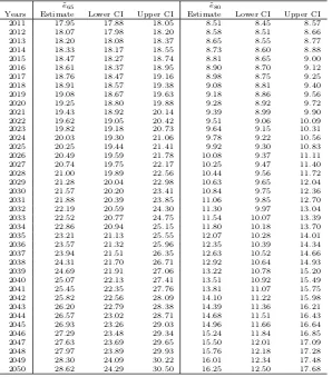
Table 2.10: Estimates and Confidence Limits of Life Expectancy at Ages 65 and 80 as Predicted by the MCH Function for US Females, 2011–2050

˜

e65 ˜e80

Years Estimate Lower CI Upper CI Estimate Lower CI Upper CI 2011 17.95 17.88 18.05 8.51 8.45 8.57 2012 18.07 17.98 18.20 8.58 8.51 8.66 2013 18.20 18.08 18.37 8.65 8.55 8.77 2014 18.33 18.17 18.55 8.73 8.60 8.88 2015 18.47 18.27 18.74 8.81 8.65 9.00 2016 18.61 18.37 18.95 8.90 8.70 9.12 2017 18.76 18.47 19.16 8.98 8.75 9.25 2018 18.91 18.57 19.38 9.08 8.81 9.40 2019 19.08 18.67 19.63 9.18 8.86 9.56 2020 19.25 18.80 19.88 9.28 8.92 9.72 2021 19.43 18.92 20.14 9.39 8.99 9.90 2022 19.62 19.05 20.42 9.51 9.06 10.09 2023 19.82 19.18 20.73 9.64 9.15 10.31 2024 20.03 19.30 21.06 9.78 9.22 10.56 2025 20.25 19.44 21.41 9.92 9.30 10.83 2026 20.49 19.59 21.78 10.08 9.37 11.11 2027 20.74 19.75 22.17 10.25 9.47 11.40 2028 21.00 19.89 22.56 10.44 9.56 11.72 2029 21.28 20.04 22.98 10.63 9.65 12.04 2030 21.57 20.20 23.41 10.84 9.75 12.36 2031 21.88 20.39 23.85 11.06 9.85 12.70 2032 22.19 20.59 24.30 11.30 9.97 13.04 2033 22.52 20.77 24.75 11.54 10.07 13.39 2034 22.86 20.94 25.15 11.80 10.18 13.70 2035 23.21 21.13 25.55 12.07 10.28 14.01 2036 23.57 21.32 25.96 12.35 10.39 14.34 2037 23.94 21.51 26.35 12.63 10.52 14.66 2038 24.31 21.70 26.71 12.92 10.64 14.93 2039 24.69 21.91 27.06 13.22 10.78 15.20 2040 25.07 22.13 27.41 13.51 10.92 15.49 2041 25.45 22.35 27.76 13.81 11.07 15.75 2042 25.82 22.56 28.09 14.10 11.22 15.98 2043 26.20 22.79 28.38 14.39 11.36 16.21 2044 26.57 23.02 28.71 14.68 11.51 16.43 2045 26.93 23.26 29.03 14.96 11.66 16.64 2046 27.29 23.48 29.34 15.24 11.84 16.85 2047 27.63 23.69 29.65 15.50 12.01 17.09 2048 27.97 23.89 29.93 15.76 12.18 17.28 2049 28.30 24.09 30.22 16.01 12.34 17.48 2050 28.62 24.29 30.50 16.25 12.50 17.68

Tables 2.11 and 2.12 show the out-of-sample statistics and DM test results for forecasting given

the prescribed forecast periods with the LC model and the MCH function for males and females.

The tables show that the proposed methodology has better out-of-sample performance in most

cases, particularly at ages 0 and 80, for both males and females. In these tables, the MCH function

performs well over the LC model for all ages for both the MAE with the MCH function having

lower values and the DM test indicating that the LC has larger errors than the MCH. In-sample

results are shown in Tables 2.13 and 2.14. The LC model has better fit in-sample, but this may

be a sign of overfitting the data.

Table 2.11: Out-of-Sample Statistics for 10-Year Forecasts, US Males

Age MAE DM Test (LC-MCH)

LC MCH Statistic P-Value