Studies on real world visual field data in glaucoma

(1)

City, University of London Institutional Repository

Citation

: Saunders, L. J. (2015). Studies on real world visual field data in glaucoma.

(Unpublished Doctoral thesis, City, University of London)

This is the accepted version of the paper.

This version of the publication may differ from the final published

version.

Permanent repository link:

http://openaccess.city.ac.uk/16170/

Link to published version

:

Copyright and reuse:

City Research Online aims to make research

outputs of City, University of London available to a wider audience.

Copyright and Moral Rights remain with the author(s) and/or copyright

holders. URLs from City Research Online may be freely distributed and

linked to.

City Research Online: http://openaccess.city.ac.uk/ [email protected]

(2)

1

Studies on real world

visual field data in

glaucoma

Luke John Saunders

A thesis submitted for the degree of Doctor of

Philosophy

(3)

City, University of London Northampton Square London EC1V 0HB United Kingdom

T +44 (0)20 7040 5060

www.city.ac.uk Academic excellence for business and the professions

THE FOLLOWING PART OF THIS THESIS HAS BEEN PUBLISHED:

Work in Chapter 4 has been published as the following article:

Saunders, L.J., Russell, R.A. and Crabb, D.P., (2015). Measurement

Precision in a Series of Visual Fields Acquired by the Standard and Fast

Versions of the Swedish Interactive Thresholding Algorithm: Analysis of

Large-Scale Data From Clinics,

JAMA Ophthalmology, 133

(1): 74-80.

(4)

2

List of Tables

Table 1.1 – Methods of detecting glaucomatous progression. ... 54

Table 2.1 - Patient information and Mean Deviations (MDs) of the cohort. ... 78

Table 3.1 - The demographics of patients analysed in the study. ... 92

Table 3.2 - The proportion of patients likely to suffer visual field impairment in the course of their lifetime ... 94

Table 4.1 – Characteristics of Study Sample ... 109

Table 4.2 - Time to detect progression at p < 0.01 for SITA Standard and Fast using

simulations of 100,000 progressing thresholds ... 112

(9)

7

List of Figures

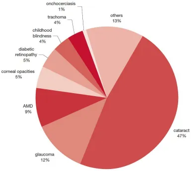
Figure 1.1 – Global causes of blindness due to eye disease; glaucoma is the second leading cause of blindness worldwide. The figure was reproduced from

http://www.who.int/whr2001/2001/archives/2000/en/pdf/StatisticalAnnex.pdf accessed in June 2014. ... 19

Figure 1.2 – A flow-chart showing the prevalence of different classifications of glaucoma. Pseudoexfoliative and pigmentary glaucoma are classed as secondary glaucomas. Diagram recreated based on figure 7.1 from Henson 2000 ... 21

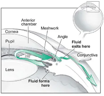
Figure 1.3 - The fluid pathway in the eye. Glaucoma is often related to the partial or complete blockage of the outflow of aqueous fluid through the trabecular meshwork (labelled “meshwork”). The “angle” refers to the angle between the iris and cornea. In open-angle glaucoma this is wide, whereas in angle-closure glaucoma this is narrow such that the iris presses against the cornea. Image taken from the National Eye Institute: http://www.nei.nih.gov/health/glaucoma/glaucoma_facts.asp accessed in June 2014. . ... 22

Figure 1.4 – Output from an OCT showing the Retinal Nerve Fibre Layer of my own right eye. ... 27

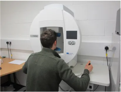
Figure 1.5 – A colleague performing Standard Automated Perimetry on an Octopus Visual Field device ... 30

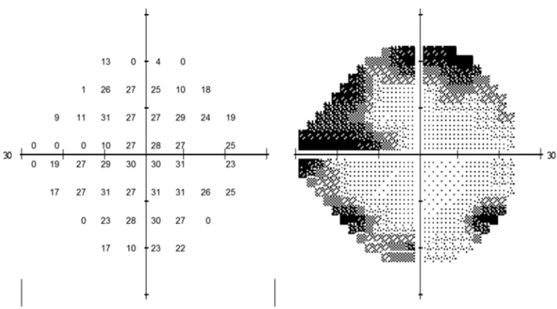
Figure 1.6 – Output from a Visual Field (VF) examination from a patient’s right eye. The left grid shows the measured threshold sensitivities at 52 locations (excluding the blind spot), whereas the right grid is a greyscale with darker areas representing less sensitive parts of the VF. ... 31

Figure 1.7 – The mean sensitivities for Full threshold, SITA Standard and SITA Fast tests taken on the same patients in a study by Artes et al. 2002. SITA Fast and Standard tests tended to yield higher, more optimistic thresholds than full threshold testing. Image taken from Artes et al. 2002. ... 34

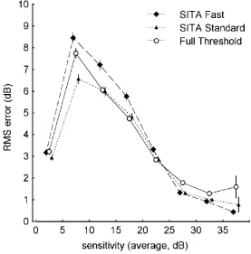
Figure 1.8 – The test-retest variability about full-threshold measured thresholds using Full threshold, SITA Standard and SITA Fast VF testing. The variability is greater for SITA Fast than Full threshold, but SITA Standard performs relatively well by comparison. This image is taken from Artes et al. 2002... 35

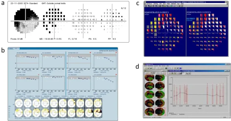
Figure 1.9 – A range of analytical tools available for use in clinical practice a) Statpac 2’s Glaucoma Probability Analysis for the HFA, b) Eyesuite Analysis software for the Octopus perimeter, c) Progressor and d) Peridata’s boxplot trend analysis ... 39

(10)

8

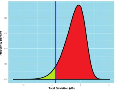
Figure 1.11 - The above distribution represents the variation in the total deviation value (TD) of a given point in a monocular VF. If a measured TD value falls within the green area (i.e. below the fifth percentile), then there is a significant probability of damage and the location will be flagged in the TD plot. This figure was previous published in the European Ophthalmic Review (Saunders et al. 2013). ... 42

Figure 1.12 – Total and Pattern Deviation plots. The top grids show the number of decibels that each threshold deviates from the expected threshold, whereas the bottom grids show the percentiles of the estimated distribution of a normal population the thresholds reside below. Pattern deviation plots correct for diffuse loss in the eye that often results from cataract; a common co-morbidity in old age... 43

Figure 1.13 - A demonstration of the differences between (a) event and (b) trend based analyses for one point in consecutive visual fields (VF). ... 51

Figure 1.14 – An illustration of how variability changes with sensitivity levels in various clinical studies. This figure was taken from Russell et al. 2012a. ... 56

Figure 1.15 – Based on Table 2 in the paper by Chauhan et al. 2008b, this graph shows an estimate of the number of visual fields per year required to have an 80% probability of successfully detecting a progressive change in mean deviation in a given number of years. This figure was first published in the European Ophthalmic Review (Saunders et al. 2013).58

Figure 1.16 – The print-out from an Esterman Test taken from Viswanathan et al. 1999. .. 62

Figure 1.17 - This figure illustrates how the integrated visual field (IVF) is calculated. Corresponding points in the left and right visual fields (VF) are compared and the one with the higher sensitivity is chosen to represent the IVF for that point. The nasal steps are unique to each eye so these are not used in the IVF. ... 64

Figure 1.18 – Findings taken from the Murata et al. 2013 study showing the different parts of the visual field (VF) important in A) Reading, B) Walking, C) Dining and D) Going out. Image was taken from Murata et al. 2013. ... 69

Figure 1.19 – An illustration of the conundrum associated with monitoring visual field loss over time. The aim of glaucoma management is to prevent patients from reaching a state of severe visual impairment within their lifetime, yet it is not clear when patients have progressed to blindness. This figure is based on an image from the European Glaucoma Society Guidelines ... 71

(11)

9

Figure 2.1 - A receiver operating characteristic (ROC) plot for using different summary measures for predicting the IVF surrogate measure of legal fitness to drive. ... 79

Figure 2.2 - A schematic showing the relationship between defect levels (better eye mean deviation) and the probability of failure of the surrogate Esterman test with 95%

confidence intervals (CI). ... 80

Figure 2.3 - Examples of ‘true-positive’ (A), ‘true-negative’ (B), positive’ (C) and ‘false-negative’ (D) patients ... 82

Figure 3.1 - A schematic illustrating the analysis conducted in this study. Visual field (VF) series from the left and right eyes of a patient were used to estimate a linear rate of loss in each eye (dB/y). The patient’s median life expectancy was obtained from the UK Office of National Statistics and was used to predict the mean deviation (MD) of each eye at

expected time of death. ... 89

Figure 3.2 (A) Distribution of residual life expectancies for all 3790 patients included in the study and (B) the rate of progression of Mean Deviation (decibels per year) from all 7149 eyes ... 93

Figure 3.3 - A series of scatterplots showing Mean Deviation (MD) in vertical (Y-axis) and horizontal (X-axis) eyes at baseline, at the end of follow-up and, through extrapolating current rates of MD deterioration, after 10, 20 and 30 years follow-up and at the end of expected lifetime. Both eyes in the plot had to fulfil the original inclusion criteria. ... 96

Figure 4.1 - Back-to-back histograms showing distributions of the frequency density of raw residuals generated through linear modelling of each test location at rounded fitted values of 0, 10, 15, 20 and 30dB for SITA Standard (grey) and SITA Fast (red). ... 110

Figure 4.2 - Variability across sensitivities for SITA Standard (grey) and Fast (red)... 111

Figure 4.3 - Simulated greyscales produced from a baseline real life visual field of the same eye, but the variability from SITA Standard and Fast using R statistical software. Each test location was simulated to progress at 2dB per year with noise added from the distributions of residuals for each fitted sensitivity. ... 113

Figure 5.1 – An optic nerve – the solid and dashed lines show the locations of the alpha and Beta-zones respectively. Damage to retinal pigment epithelial cells in this area is defined as Beta-zone parapapillary atrophy. This image has been taken from Teng et al. 2010. . 125

Figure 5.2 – This Bland-Altman plot displays the differences between observed and

predicted rates of loss in the validation dataset taken from De Moraes et al. 2012 ... 130

(12)

10

Figure 5.4 – A histogram showing the distribution of adjusted R2 values from 100,000 simulated reference models fitted to simulated validation datasets.. ... 134

Figure 5.5 - A plot of the estimated progression rate of patients in the selected reference dataset against their “true” rate of progression ... 135

Figure 5.6 - A Bland-Altman plotcomparing the progression rates of a selected validation dataset to the rates estimated in the model shown in figure 5.5. ... 136

Figure 6.1 - A map displaying each test location in the binocular IVF ranked by R2 statistics in the Reading study discussed in section 6.3.1 Figure taken from Burton et al. 2015. ... 145

(13)

11

Acknowledgements

First and most importantly of all, I would like to thank my supervisors Professor David Crabb and Dr Richard Russell for all their support over the last three years, not least for their involvement in all of the projects contained within this thesis. David’s ideas, ambition and encouragement have been invaluable in my progression as a researcher, whilst Richard has been as much an invaluable friend as well as a supervisor and has always been around when I have needed guidance and advice. I am so grateful and indebted to them both.

I am also much obliged for the support that I have received from Moorfields Eye Hospital and for all the clinical data used in the study. In particular, I would like to thank Ted Garway-Heath an am hugely grateful for the opportunity to present my research at Moorfields Glaucoma Seminars. Andrew McNaught (Department of Ophthalmology, Gloucestershire Hospitals NHS Foundation Trust, Cheltenham and Cranfield University, Bedford), James Kirwan (Department of Ophthalmology, Queen Alexandra Hospital, Portsmouth) and Nitin Anand (Calderdale and Huddersfield NHS Foundation Trust) further deserve acknowledgement for providing access to visual field data from their respective hospitals.

This thesis would not have been possible without the funding I have received from my City University of London studentship, which has also been co-funded by an unrestricted grant from Allergan Inc. I am also highly grateful to the University for giving me so many opportunities to present my research and allowing me to receive feedback that has greatly enhanced my presentation skills.

(14)

12

(15)

13

Declaration

The work contained in this thesis was completed by the candidate, Luke John Saunders. It has not been submitted for any other degrees, either now or in the past.

Where work contained within it has been previously published, this has been stated in the text. All sources of information have been acknowledged and references have been given.

(16)

14

Abstract

Glaucoma is a leading cause of blindness. As a progressive condition, it is important to monitor how the visual field (VF) changes over time with perimetry in preventing vision from deteriorating to a stage where quality of life is affected. However, there is little evidence of how clinical measurements correlate with meaningful quality of life landmarks for the patient or, by extension, the proportion of patients in danger of progressing to these landmarks. Further, measurement variability associated with visual fields make it difficult to monitor true change over time. The purpose of this thesis was to use large-scale clinical data (almost 500,000 VFs) to address some of these issues.

The first study attempted to relate clinical measurements of glaucoma severity to UK legal fitness to drive status. Legal fitness to drive (LFTD) was estimated using the integrated visual field as a surrogate of the Esterman test, which is the approved method by the UK DVLA of defining LFTD, while the mean deviation (MD) was used to represent defect severity. An MD of -14dB or worse in the better eye was found to be associated with a 92% (95% Confidence Interval [CI]: 87-95%) probability of being legally unfit to drive.

The second study used a statistical model to estimate the number of patients progressing at rates that could lead to this landmark of significant visual impairment or blindness in their predicted remaining lifetime. A significant minority of patients were progressing at rates that could lead to statutory blindness, as defined by the US Social Security Administration, in their predicted remaining lifetime (5.2% [CI: 4.5-6.0%]) with a further 10% in danger of becoming legally unfit to drive (10.4% [CI: 9.4-11.4%]). More than 90% (CI: 85.7-94.3%) of patients predicted to progress to statutory blindness had an MD worse than -6dB in at least one eye at presentation, suggesting an association between baseline VF damage and risk of future impairment.

The next section investigated whether choice of testing algorithm, SITA Standard or SITA Fast, affected the time taken to detect progression in VF follow-up. The precision of the tests was measured using linear modelling techniques and the impact of these differences was analysed using simulations. Though SITA Fast was found to be slightly less precise, no evidence was found to suggest that this resulted in progression being detected later.

The final study evaluated a validated and published risk calculator, which utilised baseline risk factors to profile risk of fast progression. A simpler model using baseline VF data was developed to have similar statistical properties for comparison (including equivalent R2 statistics). The results suggested that risk calculators with low R2 statistics had little utility for predicting future progression rate in clinical practice.

(17)

15

List of Abbreviations and Terms

ACG Angle closure glaucoma

ADREV Assessment of Disability Related to Vision AGIS Advanced Glaucoma Intervention Study AIGS Advanced Imaging in Glaucoma Study

ANSWERS Analysis with Non-Stationary Weibull Error Regression with spatial enhancement

AUC Area Under the curve

Beta-PPA Beta-zone Parapapillary Atrophy BEMD Better Eye Mean Deviation CCT Central Corneal Thickness CGS Canadian Glaucoma Study CI Confidence Interval

CIGTS Collaborative Initial Glaucoma Treatment Study CNTGS Collaborative Normal Tension Glaucoma Study CPSD Corrected Pattern Standard Deviation

DH Disc Haemorrhage

DVLA Driving and Vehicle Licensing Agency EMGT Early Manifest Glaucoma Trial ERF Error Related Factor

FDP Frequency Doubling Perimetry FDT Frequency Doubling Technology FL Fixation losses

FN False negative FP False positive

(18)

16

HFA Humphrey Field Analyzer IOP Intraocular Pressure IVF Integrated Visual Field IQR Interquartile Range LFTD Legal Fitness to Drive LFTDP Legally Fit to Drive Patients LUTDP Legally Unfit to Drive Patients MD Mean Deviation

NICE National Institute for Health and Clinical Excellence NPV Negative Predictive Value

NTG Normal Tension Glaucoma

NY-GAPS New York Glaucoma Progression Study OHT Ocular Hypertension

OHTS Ocular Hypertension Treatment Study OLSR Ordinary Least Squares Regression ONH Optic Nerve Head

ONS Office of National Statistics OPP Ocular Perfusion Pressure

PoF Probability of failure (the positive predictive value) PD Pattern deviation

PLR Pointwise Linear Regression POAG Primary open angle glaucoma PSD Pattern Standard deviation POAG Primary Open Angle Glaucoma PROM Patient Reported Outcome Measure QoL Quality of Life

(19)

17

SITA Swedish Interactive Thresholding Algorithm SSI Severely Sight Impaired

SWAP Short-wavelength automated perimetry TD Total deviation

UKGTS United Kingdom Glaucoma Treatment Study

USP-GVFSS University of Sao Paulo Glaucoma Visual Field Staging System VF Visual Field

VFI Visual Field Index

WEMD Worse Eye Mean Deviation

(20)

18

Chapter One:

Background and Aims

This introductory chapter sets out to briefly go over the important background information underpinning my topic and defining the research questions that I have set out to answer in this thesis. It begins by briefly describing what glaucoma is, the risk factors associated with its incidence and progression and the way that a patient visual field (VF; this refers to the full extent of what an eye can see) is measured. The importance of monitoring loss effectively over time, the means of doing so and the problems associated with this VF loss will also be looked at, thus, setting the groundwork necessary to introduce how the work in this thesis contributes to current clinical understanding.

1.1 Glaucoma

(21)

19

Figure 1.1 – Global causes of blindness due to eye disease; glaucoma is the second leading cause of blindness worldwide. The figure was reproduced from

http://www.who.int/whr2001/2001/archives/2000/en/pdf/StatisticalAnnex.pdf

accessed in June 2014.

[image:21.595.115.500.71.416.2]

(22)

20

(23)

21

Figure 1.2 – A flow-chart showing the prevalence of different classifications of glaucoma. Pseudoexfoliative and pigmentary glaucoma are classed as secondary glaucomas. Diagram recreated based on figure 7.1 from Henson 2000

(24)

22

[image:24.595.123.474.156.480.2]

fact that there is not yet any cure for the blindness caused by it, makes finding ways of detecting and preventing the disease progression imperative.

Figure 1.3 - The fluid pathway in the eye. Glaucoma is often related to the partial or complete blockage of the outflow of aqueous fluid through the trabecular meshwork (labelled “meshwork”). The “angle” refers to the angle between the iris and cornea. In open-angle glaucoma this is wide, whereas in angle-closure glaucoma this is narrow such that the iris presses against the cornea. Image taken from the National Eye Institute:

http://www.nei.nih.gov/health/glaucoma/glaucoma_facts.asp accessed in June 2014.

1.1.1 Risk factors in glaucoma

(25)

23

case in patients with NTG), it has been shown repeatedly to not only be a major risk factor for glaucomatous disease incidence and progression (Sommer et al. 1991, Gordon et al. 2002, Chauhan et al. 2008a, Kim et al. 2011, Jiang et al. 2012), but also a factor in the rate of progression of the disease (Heijl et al. 2012a, Medeiros et al. 2012, Chauhan et al. 2014). Large fluctuations in IOP have also been demonstrated to be a risk factor for glaucoma (Asrani et al. 2000, De Moraes et al. 2011a). How pressure relates to the death of ganglion cells is not fully understood, but its effects, along with the fact it can be changed, makes it an essential risk factor to consider.

(26)

24

explanation is down to the fact that thicker corneas tend to give higher IOP readings using tonometry than individuals with thinner corneas.

There are various other suspected factors that are not universally acknowledged as risk factors for disease. For instance, increased systolic blood pressure has been linked to disease incidence (Jiang et al. 2012) whilst other morbidities such as diabetes (Mitchell et al. 1997, Gordon et al. 2002), vasospastic disease (Broadway & Drance 1998) and even sleep apnoea (Mojon et al. 2000) have all previously been linked, although their relationships with the disease is by no means proven (Chauhan et al. 2008a, European Glaucoma Prevention Study Group 2007). Ocular perfusion pressure (OPP) is another clinical characteristic that has previously been linked to developing glaucoma (Leske et al. 2008, Zheng et al. 2010), largely in an attempt to explain why not every glaucoma patient has high IOP. However, ocular blood flow is difficult to measure and has largely been estimated using a function of the blood pressure and IOP. Unfortunately, this measurement does not give any more information than blood pressure where IOP is also being accounted for (Khawaja et al. 2013). As a result, the status of OPP as an independent risk factor is still questionable.

1.1.2 Diagnosis of glaucoma

Glaucoma is diagnosed through using a battery of different tests: National Institute for Health and Clinical Excellence (NICE) Guidelines stipulate that all people suspected of having POAG or who even have OHT should have Goldmann applanation tonometry performed, CCT measured using pachymetry, gonioscopy performed, VF measurements using standard automated perimetry (SAP) and optic nerve head (ONH) assessment using stereoscopic slit lamp biomicroscopy (National Institute for Health and Clinical Excellence 2009).

(27)

25

treatment severity (National Institute for Health and Clinical Excellence 2009). The ONH assessment allows clinicians to look at the health of the optic nerve, but SAP is the only means of directly investigating the actual visual health in terms of its impact on the patient. Due to its importance in assessing disease status and its relevance to the patient, it is measurements from SAP that will be predominantly looked at over the course of this thesis.

1.1.3 Treatment for glaucoma

Whilst, these risk factors are all related to glaucoma and could be useful for consideration in screening purposes, controlling the IOP remains the only means of treating the disease. Various clinical trials, including the Ocular Hypertension Treatment study (OHTS) (Gordon et al. 2002), the Early Manifest Glaucoma Trial (EMGT) (Heijl et al. 2002, Leske et al. 2003) and the Canadian Glaucoma Study (CGS) (Chauhan et al. 2010) have all demonstrated the utility of lowering the IOP to reduce the incidence and progression of glaucoma.

Management of IOP is performed either through medication (normally eye drops), laser treatment or surgery. Eye drops are certainly preferable, but can have various side-effects ranging from eye irritation to nausea. Non-adherence to treatment is a large issue in glaucoma (Gurwitz et al. 1993, Shaw 2005) for various reasons, including the fact that patients do not realise their vision is getting worse and therefore the importance of adherence. In addition, treatments can also be difficult to administer, particularly for elderly patients, who are unfortunately also the main demographic affected by glaucoma.

(28)

26

surgery than lose vision (Bhargava et al. 2006), it must be taken into consideration that treatment tends to become more unpleasant as severity increases. For instance, trabeculectomy can potentially result in increased risk of cataract, infection, blurred vision, bleeding, sudden, permanent loss of central vision and even secondary glaucoma if fluid drainage is prevented by scarring.

1.2 Monitoring glaucomatous vision loss

It is clearly highly important to monitor patient visual deterioration over time in order to evaluate whether or not treatment is required or needs to be escalated (Heijl 2013). The next section will briefly look at ways of doing so in clinical practice.

1.2.1 Structural measurements

(29)

27

[image:29.595.114.519.144.380.2]

2011). They are, nonetheless, useful tools in glaucoma diagnosis and monitoring when used alongside more functional means of measuring glaucomatous loss. However, this thesis will not focus on the use of these measurements.

Figure 1.4 – Output from an OCT showing the Retinal Nerve Fibre Layer of my own right eye.

1.2.2 Perimetry

Measuring the functional progression of the glaucoma (that is, what the patient can actually see) is important in diagnosing glaucoma and monitoring its progression. Perimetry is the means by which the VF; of a patient is mapped (Henson 2000), and the only means of measuring functional progression. Other than reduction in IOP (which is the basis by which most new therapies are evaluated), VF measurements are the only accepted endpoints in the evaluation of new treatments for glaucoma; the Advanced Glaucoma Intervention Study (AGIS), Collaborative Initial Glaucoma Treatment Study (CIGTS) and EMGT being examples of major trials in which VF progression was the chief endpoint.

(30)

28

doing this were performed including the Goldmann perimeter, but these approaches have largely been superseded by automated perimetry due to the fact that Goldmann perimetry is highly dependent on the examiner in terms of accuracy and bias. Given Goldman perimetry involves a moving stimulus, patients undertaking this test tend to lose fixation to a greater extent than those using automated perimetry where the pseudo-randomised location of the stimulus is less predictable (Heijl & Krakau 1977). Thus, static automated perimetry is a clinical gold standard in clinical practice as the more reliable and more reproducible option (Fankhauser et al. 1977), although Goldmann perimetry can sometimes still be used in cases where patients struggle to interface with automated perimetry.

1.3 Standard Automated Perimetry

(31)

29

There are three main machines used for SAP in the UK at present: the Humphrey Visual Field Analyzer (HFA; Carl Zeiss Meditec, Dublin, CA), the Octopus (Haag-Streit, Köniz, Switzerland) and the Henson (Elektron technology, Cambridge, UK). These three devices produce slightly different outputs, but generally perform the same function, to similar standards. The HFA is most commonly used in many large clinical centres in the UK, especially in a tertiary or referral setting where the goal is to monitor VFs in patients with glaucoma or who are at risk of developing glaucoma.

1.3.1 Measuring the Visual Field using Standard Automated Perimetry

(32)

[image:32.595.113.525.70.381.2]

30

Figure 1.5 – A colleague performing Standard Automated Perimetry on an Octopus Visual Field device

(33)

[image:33.595.116.518.74.297.2]

31

Figure 1.6 – Output from a Visual Field (VF) examination from a patient’s right eye. The left grid shows the measured threshold sensitivities at 52 locations (excluding the blind spot), whereas the right grid is a greyscale with darker areas representing less sensitive parts of the VF.

In theory, patients will always see stimuli brighter than a test location’s threshold, but fail to see a stimulus dimmer than a location’s threshold. However, in reality, when a light brightness is presented at a level close to an individual’s true threshold, there is a chance the patient may not respond as expected. In other words, there is a probability of a patient failing to register the stimulus even if it is visible to detect. The probability of a patient seeing or not seeing a given stimulus is therefore sometimes referred to as the frequency of seeing. The aim of testing is to try and find a light threshold at which a stimulus is seen 50% of the time.

1.3.2 Perimetric Testing algorithms

(34)

32

intensity is then decreased or increased back in steps of 2dB until the patient response changes once more (the second reversal). An average of the final and penultimate test sensitivities is recorded as the threshold for that test location. The order of the VF locations tested is randomised automatically in order to aid fixation (Heijl & Krakau 1975). Ultimately, this method is thorough, but it can also take a relatively long time to complete (about 10 to 15 minutes for each eye for a 24-2 test pattern) (Bengtsson & Heijl 1998a, Bengtsson & Heijl 1998b, Nordmann et al. 1998, Wild et al. 1999) during which it can be difficult for the patient to maintain their attention. As a result, it is not suitable for all patients.

Though, in theory, the increased amount of testing is supposed to improve test precision, some researchers speculate that the resulting fatigue from the length of a full threshold testing could exaggerate defects or even result in the finding of defects that do not exist (Bengtsson & Heijl 1998b, Turpin & McKendrick 2011). Thus, faster methods have been devised in order to reduce test time. The most successful and most widely adopted of these techniques is known as the Swedish Interactive Thresholding Algorithm (or SITA as it is commonly known) for the HFA. This Bayesian technique relies on a similar principle to the full threshold methods, but seeks to cut out the unnecessary testing time by reducing the number of presentations (Bengtsson et al. 1997a).

(35)

33

to “predict” the probability of seeing a threshold for the others, so each test is actively changing the predicted threshold of the other points. A second reversal only occurs if the difference between adjacent point thresholds is larger than a pre-calculated value based on the patient’s demographic known as the error related factor (ERF) (Bengtsson et al. 1997a). The exact details of how the ERF is calculated have not been disclosed, but it is calculated automatically by most perimetry machines. During the test, response times are continually recorded and used to adjust the duration of test presentations. At the end of the test, thresholds may be adjusted slightly in post-processing according to thresholds of adjacent test locations and changes in reaction times during the test.

(36)

[image:36.595.116.450.79.329.2]

34

Figure 1.7 – The mean sensitivities for Full threshold, SITA Standard and SITA Fast tests taken on the same patients in a study by Artes et al. 2002. SITA Fast and Standard tests tended to yield higher, more optimistic thresholds than full threshold testing. Image taken from Artes et al. 2002.

(37)

35

[image:37.595.116.393.194.475.2]

sensitivity in identifying VF defects than full threshold testing and SITA Standard and there is some evidence that the results from this test are less repeatable (Artes et al. 2002) (Figure 1.8). It is uncertain whether the potential for increased testing and the impact on fatigue compensate for the natural reduction in precision as a result of less testing.

Figure 1.8 – The test-retest variability about full-threshold measured thresholds using Full threshold, SITA Standard and SITA Fast VF testing. The variability is greater for SITA Fast than Full threshold, but SITA Standard performs relatively well by comparison. This image is taken from Artes et al. 2002.

1.3.3 Reliability Indices

In an ideal world, perimetry should produce accurate results on every occasion, but results that are not reflective of a patient’s actual VF can be produced, due to loss of attentiveness, inexperience, overenthusiasm or not fixating on the central point well enough. It is therefore important to evaluate the reliability of the VFs measured before using them to inform clinical decision making.

(38)

36

fixation losses (FL). False positives are a measure of how ‘trigger-happy’ the patient is, measuring how likely they are to indicate observation of a stimulus without seeing it. In full threshold testing they are tested through simply having occasions where the device pretends to change the stimulus location, but shows no light. To cut testing times, the SITA algorithms do not use catch trials, but judge false positives by the reaction speed of the patients, such as when a subject responds before they have had time to see and react to the stimulus. False negatives are a measure of inattentiveness of the patient – the devices show a light in an area where testing has already confirmed the threshold and give a brightness that the patient should be able to detect. Fixation losses meanwhile test how accurately the subject is fixating at the fixation target by presenting stimuli at the location of their physiological blindspot; this is the area corresponding to their optic disc, which has no photoreceptors.

The major clinical trials, such as AGIS, CIGTS and EMGT have used all these measures to assess field reliability (The Advanced Glaucoma Intervention Study Investigators 1994, Gillespie et al. 2003, Heijl et al. 2008), yet the criteria applied to them remain arbitrary and vary between trials. For instance, for the AGIS and CIGTS trials, a scoring system was used which meant that patients could theoretically pass with false positive or negative rates in excess of 33% (The Advanced Glaucoma Intervention Study Investigators 1994, Gillespie et al. 2003), whilst EMGT trials did not look at the FN rate at all (Heijl, Bengtsson et al. 2008). In addition, other reliability criteria such as the total number of questions asked (The Advanced Glaucoma Intervention Study Investigators 1994) (longer tests imply greater uncertainty in measuring the threshold) and short term fluctuation values have been used (The Advanced Glaucoma Intervention Study Investigators 1994, Gillespie et al. 2003).

(39)

37

However, there were indications in the same study that this relationship was most likely to be due to a significant association between FNs and VF loss (Bengtsson 2000). Similarly, Shao et al. found FNs to be the best index for predicting test reproducibility accounting for severity of VF loss, but also found that none of the reliability indices are good predictors of overall test-retest variability (Shao et al. 2011). Montolio et al. meanwhile, found false positives to be the most crucial index, with each 10% increase in FPs being estimated to increase threshold estimates by 1dB (Junoy Montolio et al. 2012). Fixation losses have been shown to contribute to test variability without being a major contributor (Henson et al. 1996, Junoy Montolio et al. 2012).

Overall, there is likely no single “best” reliability index in assessing progression; if a VF is unreliable in any way then this has the potential of hindering the ability to detect progression, whether it gives the impression that the patient’s VF is better or worse than in reality, thereby leading to impaired clinical judgement. For this reason, clinicians should be aware reliability indices when taking VFs. Additionally, the instructions given to the patient, the correction of spherical ammetropia and patient attention may also have a significant bearing on the result and these indices should not be relied upon exclusively (Chauhan et al. 2008b).

1.3.4. Problems in monitoring Visual Field deterioration in perimetry

(40)

38

Measuring a threshold where a patient can only see 50% of presentations can often be hard to find explicitly. Using a technique called method of constant stimuli to measure stimuli accurately (Laming & Laming 1992), Gardiner and colleagues found that some locations with measured thresholds using SAP did not have a stimulus intensity associated with them that could be seen 50% of the time, which led them to conclude the probability of seeing a stimulus did not increase appreciably regardless of how bright the stimulus was at measured ‘thresholds’ of below 19dB (Gardiner et al. 2014). In other words, they concluded that the likelihood of response at 19dB or brighter is governed by chance rather than giving any information on the retinal sensitivity at that location. If this is true, then perhaps there is an argument for incorporating a new lower limit for sensitivities in VF testing (e.g. setting 20dB as the lowest possible measurement), which would perhaps reduce variability in the calculation of progression indices. In the studies included in this thesis, however, it is assumed that there is still some information to be gained from lower threshold values in VF testing.

Furthermore, the psychophysical nature of the tests means that learning effects need to be taken into consideration, as patients often improve in their ability to participate in perimetric testing with experience (Wild et al. 1989, Heijl et al. 1989, Heijl & Bengtsson 1996). As a result, measured thresholds tend to increase over time, sometimes persisting long after the first three tests (Wild et al. 1989). As the first test is often particularly deflated (one previous study reported an average increase of as much as 2.6dB in MD between the first two tests in perimetry naïve glaucoma patients [Heijl & Bengtsson 1996]), discounting the first VFs remains good practice when assessing glaucoma progression.

(41)

39

[image:41.595.115.520.151.364.2]

thorough understanding and utilisation of the available software and analysis methods to facilitate this task (Figure 1.9).

Figure 1.9 – A range of analytical tools available for use in clinical practice a) Statpac 2’s Glaucoma Probability Analysis for the HFA, b) Eyesuite Analysis software for the Octopus perimeter, c) Progressor and d) Peridata’s boxplot trend analysis

1.4. Global indices

Given the difficulty of thinking about 54 points simultaneously, it is often desirable to have a single global index to summarise the amount of vision loss in an eye. As a result, there are a range of global summary indices that have been developed for the purpose of measuring levels of VF damage.

1.4.1 The Mean Sensitivity, Mean Defect and Mean Deviation

(42)

40

This is especially pertinent given the fact that the retinal sensitivity decreases naturally with age (Heijl et al. 1987).

As a result, every type of perimeter has a normative database of VF thresholds to compare measured VF thresholds against at a given location and for a given age. Measured thresholds are then compared with these average thresholds of the rest of the population and the differences between these for each location are known as total deviations (TD). Taking the arithmetic mean of these TD values gives the mean defect (Flammer 1986). However, it is well known that the variability in the periphery of the VF tends to be higher than in the centre around the point of fixation (Heijl et al. 1987) and the mean defect does not take into account these differences. In addition, it could be argued that the more central test locations are more important in the context of patient life and therefore require greater weighting.

The most commonly used and widely understood metric for summarising damage in an individual’s VF is the Mean Deviation (MD) index (Artes et al. 2011). The MD is much like the mean defect except weighted to give more prominence to the less variable central test locations (Heijl et al. 1987). This allows for a more accurate summary of the eye’s overall visual capabilities and it is therefore commonly utilised over the mean defect.

(43)

41

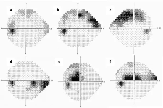
Figure 1.10 - HFA greyscale representations of six different eyes. Clearly all the VF defects are different and might impact on the patient’s day-to-day function differently. Yet all of these VFs have the same MD value of -5dB. This illustrates the limitation of using a global index, or a single number like MD to summarise the VF, because all spatial information about the defect is lost. For instance, the visual function of a patient with a central defect (such as patients e and f) is likely to be more compromised than that of a patient whose VF is affected more peripherally (such as patients a to d).

1.4.2 Total Deviation Map

Humphrey print-outs have two TD maps which show where defects in the VF are located. One is a map of measured TDs at different locations in the VF. The second is a probability map where the measured TDs are compared to the distribution of thresholds in healthy eyes (the normative database), which are annotated according to the percentile below which they fall. Thresholds measured in the bottom 5% of the sample population flagged visually with different symbols for the sub 5, 2, 1 and 0.5 percentiles (Figure 1.11). This is an effective visual way of communicating the VF of one eye when used in conjunction with the summary statistics described previously.

f e

d

c b

[image:43.595.120.462.78.306.2]

(44)

[image:44.595.128.498.82.372.2]

42

Figure 1.11 - The above distribution represents the variation in the total deviation

value (TD) of a given point in a monocular VF. If a measured TD value falls within

the green area (i.e. below the fifth percentile), then there is a significant

probability of damage and the location will be flagged in the TD plot. This figure

was previous published in the European Ophthalmic Review (Saunders et al.

2013).

1.4.3 The Pattern Deviation and Pattern Standard Deviation

(45)

43

percentile the difference between these two values are. In other words, the PD attempts to compare focal VF loss with diffuse VF loss. As with the TD plot, any readings in the bottom 10% of the population are flagged.

Figure 1.12 – Total and Pattern Deviation plots. The top grids show the number of decibels that each threshold deviates from the expected threshold, whereas the bottom grids show the percentiles of the estimated distribution of a normal population the thresholds reside below. Pattern deviation plots correct for diffuse loss in the eye that often results from cataract; a common co-morbidity in old age.

[image:45.595.117.508.145.574.2]

(46)

44

sensitivity at each field location and the normal age-normal sensitivity corrected for the patient’s MD. A high PSD thus implies that there is a great deal of variation between points measured in the VF, which is more indicative of typical glaucomatous field loss, whilst if each location is uniformly depressed (as in diffuse loss) the PSD is low. However, this measure is ineffective at the end-stage of glaucoma, because it will decrease as defects become more homogenous across the VF. Thus, the PSD not a good indicator of overall damage, though it can still be helpful when used alongside the MD (Brusini & Filacorda 2006).

1.4.4 The Visual Field Index

The Visual Field Index (VFI) is a relatively new summary measure that seeks to quantify glaucomatous damage, in later software upgrades of the HFA (Bengtsson & Heijl 2008). It is similar to the MD, though there are various notable differences. The VFI seeks to be user friendly to clinician and therefore attempts to estimate the percentage of vision the patient has left. Vision with no discernable defect is categorised at 100% with 0% signifying perimetric blindness. The VFI is weighted more towards the central VF than the MD, operating on the principle that the central part of the vision is of highest importance in terms of quality of life. Finally, the PD is utilised rather than the TD to calculate this statistic.

(47)

45

suggests that the statistic can be somewhat misleading in representing how well a patient can see (Artes et al. 2011). A possible reason behind this is that the reliance of the VFI statistic on pattern deviation is thought to fail to take into account the fact that glaucoma does also cause diffuse loss (Henson et al. 1999), which is ignored using this statistic. Thus, the VFI can risk underestimating the overall effect that glaucoma has on the eye (Artes et al. 2010) a fault also acknowledged by Bengtsson and Heijl(Bengtsson & Heijl 2008). Thus, though the VFI may potentially be useful, the MD is still a gold-standard in summarising VF loss into a single statistic.

1.4.5 Issues with global indices

Overall, though summary measures are useful in terms of having a singular measure representing how badly an individual’s vision has been degraded by glaucoma, a universal problem for all of these measures is that they waste data and ignore important spatial information. Furthermore, it is difficult to tell how changes in these measures relate to visual disability. For example, what exactly does a drop in VFI from 100 percent to 97 percent mean? Thus, criteria must be devised in order to indicate whether glaucomatous progression is taking place at a dangerous rate or not. It is also accepted that summary measures are relatively insensitive to change when subject to analysis due to the fact that it averages the healthy parts of the VF as well as the unhealthy sectors to calculate the measure deterioration (Smith et al. 1996, Wild et al. 1993).

1.5 Event and Trend-based analyses

(48)

46

result of how they treat measurements taken between the first and last VF. This gives them unique properties that have to be considered before evaluating which set of methods have the best utility in detecting glaucomatous progression.

Event based analysis involves taking a baseline and comparing every subsequent test against this reading. Any significant difference between the baseline and latest reading is considered to be due to progression. On the other hand, trend based analyses are an evolving process in which all VFs are analysed using linear regression to assess the rate and significance at which the measurement is changing.

1.5.1 Staging glaucoma patients

One means of marking progression is through using some staging system to mark when glaucomatous eyes have progressed beyond a certain level. Although useful for categorising glaucomatous eyes at diagnosis and for categorising damage in various studies, they are generally too insensitive to change to be practical in terms of monitoring progression. These methods are described in depth by Susanna Jr and Vessani (Susanna Jr. & Vessani 2009).

The most commonly used method of staging glaucoma is the Hodapp-Parrish-Anderson (H-P-A) index, which categorises defect severity into three stages (Early, Moderate and Severe) based upon MD, numbers of points below the 5% in the pattern deviation and health of points specifically in the central 5˚ (Hodapp et al. 1993). Though over 20 years old, this method of categorisation remains useful for roughly categorising VF loss and is still popular for use as a standard for VF defect severity (Elbozan Cumurcu et al. 2010, Labiris et al. 2010).

(49)

47

System (GSS), which incorporates MD and PSD to determine the stage of the defect (Brusini & Filacorda 2006). One very recent categorisation method is the University of Sao Paulo Glaucoma Visual Field Staging System (USP-GVFSS), which incorporates the VFI, the proximity of damage to fixation, the number of hemifields affected and whether the damage is connected to the blindspot into one string of code (Susanna Jr. & Vessani 2009). However, the increase in utility that has come in increasing the number of categories come at a cost of making the categorisation criteria more complex and as a result none of these methods have made a large impact in clinical practice.

1.5.2 Pointwise scoring criteria

Pointwise scoring criteria (examining each VF location separately) are sometimes used for determining progression though usually only in clinical trials, as they have good diagnostic specificity (probability of diagnosing healthy eyes as

non-progressing) (The Advanced Glaucoma Intervention Study Investigators 1994, Heijl et al. 2008, Musch et al. 1999, Heijl et al. 2003, Ernest et al. 2011, Vesti et al. 2003). Two of the most famous criteria for detecting glaucoma progression were

developed in order to analyse the results of two large scale clinical trials, AGIS and CIGTS, and hence are named after those trials.

However, both of the AGIS and CIGTS scoring methods, though specific in terms of their criteria of progression, both suffer from similar flaws to those of the summary methods described earlier. Specifically, these scoring systems can be affected and lowered by cataract, whilst there is also a fundamental loss of detail that occurs when summarising disease severity by using a single number in a disease that fundamentally affects the VF in a localised manner. As a result, in clinical practice, more sensitive event and trend based analyses tend to be utilised in order to estimate VF progression.

1.5.3 Glaucoma Change Probability Analysis

(50)

48

Probability method (GCP), which is sometimes called Glaucoma Probability Analysis or Guided Progression Analysis and is available from Statpac 2 GPA software for the HFA. This method takes the first three VFs and then averages the thresholds from the two most reliable VFs to attain a baseline reading for each test location. This baseline is compared with all subsequent VF tests and the difference between them is assessed using the GCP map, which designates the amount of variability from the average threshold one would expect from the baseline value, calculated from typical population variability. Any significant difference between the baseline and latest reading that is confirmed in two subsequent tests is considered to be due to progression and a new baseline is taken. Typically with this type of analysis, three points or more being shown as consistently defective in three tests are required to mark progression. An adapted version of the GCP map known as the pattern deviation GCP map has been used for the EMGT, which accounts for cataract based defects similarly to how the pattern deviation isolates localised effects from TD plots (Bengtsson et al. 1997b, Heijl et al. 2003).

(51)

49

patients that are exhibiting signs of progression but are consistent test-takers may not get flagged as early as they should.

1.5.4 Trend-based analyses

Event analyses are useful in determining whether progressive change is occurring, but cannot be used to predict future outcomes, which may be important in informing treatment decisions. In addition, they only tend to look at two VF observations in determining whether progression has occurred and this seems wasteful of the large amount of data collected in long term monitoring. As a result, incorporating trend-based analyses that can be used to anticipate future VF status are popular.

The simplest type of trend analysis is to monitor how summary measures change linearly over time using ordinary least squares regression (OLSR) and this is easily accessible for clinicians using software such as Statpac 2 and EyeSuite Progression Analysis software for the Octopus (Figure 1.9). Recently, this approach has been specifically advocated with the VFI in particular (Bengtsson et al. 2009), but regression of summary measures has been occasionally criticised for being relatively insensitive to measuring progression (Smith et al. 1996, Wild et al. 1993). Furthermore, summarising all of the points in the VF will tend to result in equally weighting the damaged and undamaged parts, which will inevitably not be as sensitive as concentrating on the faster progressing sections of the field. However, this approach can be nonetheless useful in giving an impression of the future status of an individual’s VF.

(52)

50

PROGRESSOR software, the results are presented in the form of a series of histograms for each point tested in the eye. Large bars represent large defects, whilst small ones represent normal vision with colours ranging from white/red (signifying significant deterioration in threshold levels) to grey (indicating no change) to green (signifying significant improvement in threshold levels). A common criterion used to assess whether progression is significant for a single point is a rate less than -1dB/year with a p-value of less than 0.01.

(53)

51

spite of the fact that assumptions of homoscedasticity (constant variability across sensitivities), normality and independence are violated (Bryan et al. 2013). Overall, linear regression is an undoubtedly imperfect, but overall an adequate compromise of fit and predictive utility in monitoring long-term VF deterioration.

1.5.5 Advantages and Disadvantages of Event and Trend-based analyses

Figure 1.13 - A demonstration of the differences between (a) event and (b) trend based analyses for one point in consecutive visual fields (VF).

In (a), each threshold is compared to the initial baseline derived from averaging two VF measurements (the first two points). If the point is significantly less than the baseline for a stable glaucomatous eye (i.e. below the dotted blue line) for three consecutive VF that point is determined as highly likely to be progressing. Only the baseline and last VFs are used to determine whether progression has occurred.

(54)

52

As a result of using all the previous fields in its diagnosis, trend analysis has distinct advantages and disadvantages compared with event based analyses. First of all, event based analyses generally require fewer VFs and less time to produce definitive results, so may detect rapid deterioration in the VF more quickly than this technique. As a result, trend analyses tend to hold a much higher risk of initially falsely diagnosing stable VFs as progressing. For example, in the scenario shown in

Figure 1.13b, progression would be diagnosed after 3-and-a-half years, but this

prognosis would change to not progressing after 4 years (though six months later progression is once again diagnosed). Conversely, trend analysis can also be slower at detecting actual glaucomatous progression than methods such as glaucoma change probability analysis (Nouri-Mahdavi et al. 2007). However, this technique estimates the rate of VF progression, which can be extremely helpful in the context of following patients continuously over a long period of time in clinical practice. Furthermore, with enough fields, trend analyses generally have higher diagnostic sensitivity than event analyses over the same time period (Vesti et al. 2003).

(55)

53

Table 1.1 on page 54 summarises the difference between various methods

(56)

54

Table 1.1 – Methods of detecting glaucomatous progression. Acronyms described in Abbreviations Section. This table has been previously published by Saunders et al. (Saunders et al. 2013)

Method Method of attaining baseline

Method of defining progression Advantages Disadvantages Correction for cataract? Method Type Rate of progression calculable? Linear Regression of MD values

No consensus, but at the very least 3 VFs are required

No consensus, but EyeSuite for the Octopus perimeter defines progression if the previous six MDs are significantly progressing (p<0.5%) (Haag-Streit

International 2009)

- Simple - No spatial consideration of the data - Assumes progression is linear

- Long time period required (Smith et al. 1996) - Low sensitivity (Smith et al. 1996)

- Affected by cataract

No Global Summary Trend Analysis Yes Linear Regression of VFI values

5 VFs over 3 years required for initial trend in Humphrey Field Analyzer software (Carl Zeiss Meditec 2008)

Assesses significance of slope, and relates rate of progression to how much VFI patients will lose in the next 5 years (Carl Zeiss Meditec 2008)

- Simple

- Gives an estimate of the % vision an individual may lose in future

- No spatial consideration of data - Assumes progression is linear - Quite a long time period required - At least 5 VF tests required - Discounts diffuse loss, so may underestimate overall glaucomatous loss

Yes Global Summary Trend Analysis Yes AGIS Method

One VF A decline in score from baseline equal to 4 “AGIS units” in 3 consecutive tests (AGIS Investigators 1994, Heijl et al. 2008)

- High specificity (Vesti et al. 2003, Heijl et al. 2008, Ernest et al. 2011)

- Score testing based on real patient data

- Poor sensitivity (Vesti et al. 2003, Heijl et al. 2008, Ernest et al. 2011)

- Cannot determine spatial characteristics of progression

- Long time required (Vesti et al. 2003) - Cannot detect progression rate - Can be affected by cataract

No Pointwise/ scoring event analysis No CIGTS Method

Two VFs (Musch et al. 1999, Gillespie et al. 2003)

A decline in score from baseline equal to 3 ‘CIGTS units’ in 3 consecutive tests (Heijl et al. 2008)

- Fast (Vesti et al. 2003)

- High specificity (Vesti et al. 2003, Heijl et al. 2008, Ernest et al. 2011)

- Score testing based on real patient data

- Low sensitivity (Vesti et al. 2003, Heijl et al. 2008, Ernest et al. 2011)

- Cannot determine spatial characteristics of progression

- Cannot detect progression rate - Can be affected by cataract

No Pointwise/ scoring event analysis

No

GCP Analysis Two VFs “Likely progression” defined as a reduction in sensitivity (below normal limits) from baseline for

≥3 separate VF points in 3

consecutive tests(Vesti et al. 2003, Heijl et al. 2008)

- Fast (Vesti et al. 2003, Nouri-Mahdavi et al. 2007)

- High sensitivity and specificity (Vesti et al. 2003, Heijl et al. 2008, Ernest et al. 2011) - Normal limits defined using real (stable) patient data

- Cannot detect progression rate - Cannot take the diffuse effects of glaucomatous loss into account

Yes Pointwise event analysis

No

PLR Analysis No consensus, but at the very least 3 VFs are required

No consensus, but usually a statistically significant (p<5%) decrease of 1dB per year for at least 3 separate VF points

- High sensitivity (Vesti et al. 2003, Ernest et al. 2011)

- High specificity (Vesti et al. 2003, Ernest et al. 2011)

- Long time period required (Vesti et al. 2003, Nouri-Mahdavi et al. 2007)

- Assumes progression is linear - Can be affected by cataract

No Pointwise trend analysis

(57)

55

1.6 Factors affecting time-to-detect progression

The most crucial aim in the monitoring of glaucoma is to diagnose VF progression as quickly as possible. Bearing this in mind, aside from criteria for flagging progression, there are three further factors that affect how quickly quality of life (QoL) threatening deterioration of the VF can be detected: the rate of VF loss, the variability in the VF series (otherwise known as the ‘noise’) and the frequency at which VF measurements are taken (Chauhan et al. 2008b).

1.6.1 Rate of loss

The rate at which VF is lost is clearly a highly important factor in the ease of detecting progression. The principle behind this is simple: if the magnitude of change in the VF from baseline is higher, then there will simply be greater power to detect a difference whatever method is used to analyse the results. However, obviously in the context of glaucoma, a more rapid rate of loss needs to be detected earlier. It is therefore important to detect deterioration in eyes progressing at a rate, which could very quickly cause visual impairment (Chauhan et al. 2008b).

1.6.2 Noise

(58)

56

glaucoma is that levels of noise increase with decreased sensitivity (Figure 1.14) (Henson et al. 2000, Artes et al. 2002, Russell et al. 2012a). Progression is therefore easier to detect in test locations with good sensitivity than locations exhibiting glaucomatous damage. Noise reaches a peak at around 10-15dB and decreases towards 0dB due to the fact that sensitivities reach the measurement’s lower limit.

Figure 1.14 – An illustration of how variability changes with sensitivity levels in various clinical studies. The blue background is a density plot of all absolute residuals taken from fitting models to retrospective visual field series in a study by Russell et al 2012a. The blue and green lines represent using least-squares linear regression and tobit regression for these field series respectively. The red and yellow lines reflect the findings of Artes et al 2002 and Henson et al. 2000 respectively. This figure was taken from Russell et al. 2012a.

1.6.3 The Frequency of Visual Field Measurements

(59)

57

variability. Gardiner and Crabb found, using simulated eyes with thresholds decreasing by 2dB per year, that undergoing three VF tests per year was optimal in terms of sensitivity and specificity of detecting progression (Gardiner & Crabb 2002b). However, their estimate of the noise is perhaps too small as it does not take into account the fact that visual thresholds are more variable in areas of lower sensitivity (Heijl et al. 1987, Henson et al. 2000, Artes et al. 2002, Russell et al. 2012a).

One of the most influential papers on this topic written by Chauhan and associates makes suggestions based on the power (the probability of correctly diagnosing a progressing patient) associated with the number of tests taken (Chauhan et al. 2008b). Chauhan et al. suggest, as a minimum, that six VFs should be taken in the patient’s first two years of monitoring, before choosing the number of subsequent tests per year on the basis of progression rate and time-scale thereafter (Figure

1.15). However, these figures are based on theoretical power calculations (using

(60)

58

Figure 1.15 – Based on Table 2 in the paper by Chauhan et al. 2008b, this graph shows an estimate of the number of visual fields per year required to have an 80% probability of successfully detecting a progressive change in mean deviation in a given number of years. This figure was first published in the European Ophthalmic Review (Saunders et al. 2013).