A comparative study of boundary conditions for lattice Boltzmann simulations of high Reynolds number flows

Contents lists available at ScienceDirect

Computers

and

Fluids

journal homepage: www.elsevier.com/locate/compfluid

Benchmark solutions

A

comparative

study

of

boundary

conditions

for

lattice

Boltzmann

simulations

of

high

Reynolds

number

flows

Kainan

Hu

a,b

_,

_Jianping

_Meng

c,∗

_,

_Hongwu

_Zhang

a

_,

_Xiao-Jun

_Gu

c

_,

_David

_R

_Emerson

c

_,

Yonghao

Zhang

d

a_{IndustrialGasTurbineLaboratory,InstituteofEngineeringThermophysics,ChineseAcademyofSciences,Beijing,China} b_{UniversityofChineseAcademyofSciences,Beijing,China}

c_{ScientificComputingDepartment,STFCDaresburylaboratory,WarringtonWA44AD,UnitedKingdom}

d_{JamesWeirFluidsLaboratory,DepartmentofMechanical&AerospaceEngineering,UniversityofStrathclyde,Glasgow,G11XJ,UK}

a

r

t

i

c

l

e

i

n

f

o

Articlehistory:

Received27June2016 Revised7June2017 Accepted13June2017 Availableonline15June2017

Keywords:

LatticeBoltzmannmethod Bounce-backscheme

Non-equilibriumbounce-backscheme Non-equilibriumextrapolationscheme Kineticboundarycondition Cavityflow

a

b

s

t

r

a

c

t

Four commonly-usedboundaryconditions inlattice Boltzmannsimulation,i.e. the bounce-back, non-equilibriumbounce-back,non-equilibriumextrapolation,andthekineticboundarycondition,havebeen systematicallyinvestigatedtoassesstheiraccuracy,stabilityandefficiency insimulatinghighReynolds numberflows.Fortheclassicallid-drivencavityflowproblem,itisfoundthatthebounce-backscheme doesnotinfluencethesimulationaccuracyinthebulkregioniftheboundaryconditionisproperly imple-mentedtoavoidgeneratingnon-physicalslipvelocity.Althoughthekineticboundaryconditionnaturally producesphysicalslipvelocityatthewall,itgivesoverallsatisfactorypredictionsofthecenter-line ve-locityprofile andthevortexcenterlocationsfortheReynoldsnumbersconsidered.Forthecavityflow problem,allfourboundaryconditionsshowminimaldifferenceinthecomputingtimeneededtoreacha steadystate.Thisissurprisingbecausethekineticboundaryconditionissignificantlydifferentfromthe otherthree schemeswhicharedesignedspecificallyforno-slipboundaryconditions.The bounce-back schemeisthemostcomputationallyefficientinupdatingboundarypoints,whichisparticularly attrac-tiveiftherearealargenumberofsolidbodiesintheflowfield.Forthenumericalstability,wefurther testthe pressure-driven channelflow withorwithoutaenclosedsquarecylinder. Overall,thekinetic boundaryconditionisthemoststableofthefourschemes.Thenon-equilibriumextrapolationscheme presentsexcellent stability secondtothe kineticboundarycondition forthe lid-drivencavity flow.In comparisonwithotherthreesschemes,thestabilityofnon-equilibriumbounce-backschemeappearsto belesssatisfactoryforbothflows.

© 2017TheAuthors.PublishedbyElsevierLtd. ThisisanopenaccessarticleundertheCCBYlicense.(http://creativecommons.org/licenses/by/4.0/)

1. Introduction

The lattice Boltzmann (LB) method has been developed into an efficient mesoscopic simulation tool for fluid dynamics [1], whichhasshownitsstrengthinsimulatingmulti-phaseand multi-component flows [2], and flows in porous media [3]. Its poten-tial for simulatinghigh Reynolds number(Re) flows has also at-tracted significantinterest. Forexample,witha second-order nu-mericalschemeinbothtimeandspace,theLBmethodwasshown to performwell for decayingturbulence,although itmay require higherspatialresolution,withacorrespondinglysmallertimestep,

∗ _{Correspondingauthor.}

E-mail addresses: hukainan@iet.cn (K. Hu), jianping.meng@stfc.ac.uk,

jpmeng@gmail.com (J.Meng),zhw@iet.cn (H.Zhang), xiaojun.gu@stfc.ac.uk (X.-J. Gu), david.emerson@stfc.ac.uk (D.R. Emerson), yonghao.zhang@strath.ac.uk (Y. Zhang).

incomparisontoaspectral method[4].However,ahigh-order LB modelhasbeensuccessfullyappliedforsimulatingtheKidavortex flow[5].Therehavebeenvariousattemptstosimulateturbulence including large eddy simulation and direct numerical simulation [6].

It isof importance to choose an appropriate boundary condi-tionforsimulatinghigh-Reflowsasitisoftenthekeytostability, efficiency,andaccuracyofsimulations,particularlyforcomplex ge-ometry[7].Conventionally,weneedtoimplementthemacroscopic no-slipboundarycondition,whichhasmanydifferent implementa-tionsintheLBmethodbecauseofitsmesoscopicnature.Themost commonly-used implementationis thebounce-back (BB) scheme, whichoriginally describesastationarywall.However,witha sim-plemodification, it canbe used formoving walls aswell [8].By assuming bounce-back of the non-equilibrium part of the distri-butionfunction,ZouandHederivedtheso-callednon-equilibrium bounce-back (NEBB)boundarycondition[9]forboth moving and

http://dx.doi.org/10.1016/j.compfluid.2017.06.008

stationarywalls. Guo et al.[10,11] proposed the non-equilibrium extrapolation(NEEP)scheme,whichisalsosuitableforboth mov-ing and stationary walls. There are also other implementations, e.g.,thecounter-slipboundary[12].

Thekineticboundarycondition(KBC)isofgreatinterestforthe LBmethod[13].Thisschemecaninducephysicallyrealisticslip ve-locityata wallboundary,andhasbeenoftenusedinthediscrete velocitymethod(DVM) [14]forrarefiedgas flows,e.g., [15].Asa specialformofDVM,theLBmethodcanalsousetheKBCto sim-ulaterarefied gasflows over a broadrange ofKnudsen numbers (Kn) [16].Moreover, theKBC hasa nicepropertyof retainingthe positivityofoutgoingparticledistributionfunctionsatthe bound-arynodesif the incomingmass flux ispositive, which is helpful fornumericalstability.Therefore,itisinterestingtoinvestigateits performanceforhigh-Reflows.

The accuracy of the BB scheme has been studied in detail for simple flows, e.g. [17,18]. It was shown that the BB scheme may induce a numerical slip velocity and cause different order oferrorsdependingonitsimplementation(e.g.,“on-grid” or “half-way”).Whilethisartificialslipvelocitycanbeeliminatedfor sim-plegeometries[19],wewillinvestigatetheperformanceoftheBB schemewithoutthedeficiency.

Other boundaryschemesarealsoassessed intheliterature in-cludingthosespecificallydesignedforcurvedboundaries(seee.g., [20–22]). Of particular interest is that the NEEP scheme shows second-order accuracy for “moderate” Reynolds number flows in complex domains [20], which is consistent with the analysis in [10,11,18] for relatively simple flows. Moreover, the scheme also presentssufficientnumericalstabilityfortheinvestigatedReynolds numbers.

In thiswork, we willfocus onaccuracy, efficiency, and stabil-ityoftheBB,NEEPNEBBandtheKBCschemes forhighReynolds numberflows.Ourbenchmarksimulationswillbeconductedusing a D2Q9 lattice model forthe classical lid-driven cavity flow and theflow around asquare cylinder confinedina channel. The re-sultswillbeparticularlyfocusedonthecavityflowwhereweare abletoassessthefourboundaryschemesforReynoldsnumbersup to7500.Fortheflowaround asquare cylinder,we willprimarily investigatetheirnumericalstability.

2. Lattice Boltzmann equation and D2Q9 lattice model

The LB methodcan be consideredasan approximation tothe Boltzmann-BGKequation [23–25].The governing equationcan be writtenas

∂

f_α

∂

t +cα·

∇

fα=−

1

τ

(

fα−f_αeq

)

. (1)

Thisequation describes the evolution of the distribution f_α

(

x,t

)

forthediscretevelocityc_α atpositionx andtime t.Thecomplex molecularinteractionissimplifiedasarelaxationschemetowards thediscreteequilibriumdistribution f_αeq

(

x,t

)

.Inordertosimulate incompressibleandisothermalflows,itiscommontousean equi-libriumfunctionwithsecond-ordervelocityterms

f_αeq=w_α

ρ

1+u·cα RT0 +

1 2

(

u·c_α

)

2

(

RT0

)

2 −

u·u

2RT0

, (2)

whichisdetermined by thedensity,

ρ

,thefluid velocity, u,,and thereferencetemperature, T0.Forgas flows, theconstant, R,can beconveniently understood asthegas constant. Ifa liquidis in-volved,R,togetherwithT0,canbeconsideredasareference quan-tity.Forconvenience,thesoundspeedcsisoftenconsideredtobe

RT0,although thereisaconstantfactor√

γ

ofdifference where

γ

istheratioofspecificheats.Theweightingfactorisdenotedby w_α forthe discrete velocity c_α.Althoughthe LB methodappears

to be a primary tool for modeling gas flow, based on its origin fromkinetic theory,it canalsobe usedforliquidflows. This uti-lizesthefactthat,underappropriateconditions,theNavier–Stokes (NS)equations can berecovered, whichis validforboth gasand liquidflows.

The relaxation time

τ

is related to the fluid viscosity via the Chapman–Enskog expansion, i.e.,

μ

₌p

τ

_, where

μ

is the vis-cosity and p the pressure. Hence, for isothermal and incom-pressible flows, the Reynolds number becomes Re=

ρ

0u0L/

μ

= u0L/

(

τ

RT0

)

,wherethesubscript0denotesthereferencevalueand L is the characteristic length of the system. It is worth noting that the important non-dimensional number, Kn, can be defined as

μ

0

RT0/

(

p0L

)

. So,

τ

is also related to the Knudsen number through viscosity, i.e., Kn=

τ

RT0/L where p0=

ρ

0RT0. We can thereforeobtainKn×Re=u0/

RT0=Ma.Forgasflows,the Knud-sennumberistheratioofthegasmeanfreepathandthe charac-teristiclength,whichmeasurestherarefiedlevelofgasflows.Ifa liquidflowissimulated,wemaynotbeabletodefineaphysically meaningful Knudsen number. However, the above defined Knud-sennumbercanberegardedasanimportant“numerical” number forLB simulationdueto itskinetic nature.In thiscase, this “nu-merical” Knudsen number will influence the dynamical behavior ofmodellingliquidflow. WhenKn becomeslarge,the LBmethod maydeviatefromtheNSdynamicssignificantly,eveninthe bulk regionawayfromanysurface[26].Therefore,forliquidflows,itis importantto ensurea small“numerical”Kn inanyLB simulation inordertoavoiddeviatingfromtheNShydrodynamics.However, thisisnota problemforgasflows. Instead,itprovidesan oppor-tunitytomodelrarefiedgasflowswithsuitablerangesofKnudsen numbers(seee.g.[16]).

Fortheisothermalcase,onlydensityandvelocityareofinterest andcanbeobtainedas

ρ

=

α

f_α,and

ρ

u= α

f_αc_α. (3)

A smartscheme can be utilized tonumerically solve Eq.(1)and achieve the particle-jump like simulation [27]. By applying the trapezoidalintegrationruleforbothsidesofEq.(1)and introduc-ingatransformation

˜

fα=fα+₂dt

_τ

(

fα−f_αeq

)

, (4)

weobtainthediscretizedformfor f˜as

˜

f_α

(

x+c_αdt,t+dt

)

−_f˜_α

₍

_x,t

₎

₌₋ dt

τ

+0.5dt

_˜

f_α

(

x,t

)

−f_αeq

(

x,t

)

,

(5)

whichprovidesthestream-collisionalgorithm.

The last key step is to choose an appropriate set of discrete velocities. The D2Q9 lattice is the mostpopular choice for two-dimensionalflows,whichemploysninediscretevelocities

c_α=

⎧

⎨

⎩

(

0,0

)

,

α

=0,

(

cos

(

α

−1

)

π

/2, sin

(

α

−1

)

π

/2

)

3RT0,

α

=1,2,3,4,

(

cos

(

2

α

−9

)

π

/4, sin

(

2

α

−9

)

π

/4

)

3RT0,

α

=5,6,7,8. (6)

The corresponding weights are w0=4/9, w1−4=1/9, w5−8= 1/36.

(i,j) (i,j+1) f1 f2 f3 f4 f5 f6

f7 f8

f0

Solid Boundary(South Wall) Fluid

Fig.1. Illustrationofsouth(bottom)wallboundary.

Table1

Parameters fortwogridsofaphysicalsystemdefinedbyu0, ν0 andT0,where

dx0=L/NisthespatialstepsizewithNcells.

cellnumber dx(dt3RT0) uˆ0 τˆ νˆ τˆo

N dx0 √u₃0_RT

0 3ν0

dx0

√

3RT0 ν0

dx0

√

3RT0 3ν0

dx0

√

3RT0

+1 2

2N dx0

2 √u₃0_{RT0 dx0}√6ν0_{3RT0 dx0}2√ν0_{3RT0 dx0}√6ν0_3RT0+12

we may transform Eq.(1) to its non-dimensional form first and thenapplytheschemegivenbyEq.(5),asdonein[26].Obviously, the non-dimensionaltransformationwill notalter thefinal simu-lationresults.

Itiscommontochoose thespacestepdxordyandtimestep dtasreferencevalues,i.e.,the“lattice” unit.FortheD2Q9model, thetransformationis

ˆ

x= x

dx, tˆ= t dt, uˆ=

u

3RT0

, cˆ_α=

cα 3RT0

,

τ

ˆ=

τ

dt, (7)

where the hat symbol is used to denotenormalized variables in thelatticeunit.Also,wenotedx=dt

3RT0.Withthe transforma-tion,Eq.(5)becomes

˜

f_α

(

xˆ+cˆ_α,tˆ+1

)

−_f˜_α

₍

_xˆ,tˆ

)

=− 1

ˆ

τ

+0.5

_˜

f_α

(

xˆ,tˆ

)

−f_αeq

(

xˆ,tˆ

)

.

(8)

Forconvenience,a newrelaxationtime

τ

ˆo₌

_τ

_{ˆ+0.5isalways} in-troduced. In addition,it isalso commonpracticeto calculatethe importantnon-dimensionalvariablesinthelatticeunit,i.e.,

Re=u0L

ν

=

ˆ

u0Lˆ ˆ

ν

, Kn=

τ

RT0 L = ˆ

τ

ˆ

L√3, (9)

where

ν

denotes the kinematic viscosity and we have

ν

₌ ˆ

ν

dx

3RT0.Thelength Lˆinthelatticeunitbecomesthecell num-ber ofone coordinateandiscommonlydenotedasN.Finally,the relation between the viscosity and relaxation time in the lattice unitis

RT0

τ

=

ν

⇒ ˆ

τ

3 =

ν

ˆ⇒ ˆ

τ

o_−0.5

3 =

ν

ˆ. (10)

While any proper transformations will not influence the final results,wefindthatanissuemayoccurwiththelatticeunitwhen conducting grid independent tests. Forconvenience, we consider isothermalandincompressibleflow.Followingtheaforementioned procedure,welistparametersinboththephysicalunitandlattice unit oftwodifferentgridsystemsinTable1.Thephysicalsystem isdefinedbyasetoffixedparametersu0,

ν

0andT0.Itshowsthat, tokeep alltheparameters exactlythesameinphysicalunits,the relaxationtimeandviscosityinthelatticeunitshoulddepend lin-earlyonthemeshsize.Itisdifferentfromthepracticewherethe viscosity

ν

ˆinthelatticeunitisfixed.From theabove transforma-tion and Table 1, if

ν

ˆ andRe are fixed, the corresponding

phys-ical systemneeds to have eithera different viscosityor a differ-entcharacteristiclength whilethecharacteristicvelocity mustbe changed.Thisturnsouttobe,however,inconsistentwithcommon CFDpractice.Infact,sincebothMaandKnarechangedinthisway, thereisarisk thatKnforthecoarsestmeshbecomessolarge(cf. Eq.9)thattheLBmethodmaydeviatefromtheNSdynamics,even inthebulk [26].Forthisreason,weshallkeepall theparameters unchangedinphysicalunitsforgridindependenttestsorscheme accuracyanalysis.

3. Numerical assessment of various boundary conditions

3.1. Boundaryconditions

WechoosetodiscusstheKBCandtheBB,NEBB,NEEPschemes, andtheirimplementationisillustratedinFig.1.Foranyboundary scheme, the aim is to determine the outgoing distribution func-tions fb

5, f2b and f6b, where the superscript b is used to denote boundary point,according to the incomingdistribution functions

fb

7, f4band f8bknownfromthestreamstep.Itisworthnotingthat we will use the “on-grid” implementation for all four boundary conditions.

The main idea ofthe BB scheme is that an incoming particle distributiondirecting to thewall bounces back intothe fluid do-mainintheoppositedirection.Therefore,fortheD2Q9model,we have fb

5=f7b, f2b= f4b and f6b= f8b. Asdiscussed in[19],the non-physicalslipvelocitycan beeasily eliminated forthiscavityflow bytakingcareof fb

1 and f3b.

TheKBC assumesthat an outgoing particlecompletely forgets itshistoryanditsvelocityisrenormalizedby theMaxwellian dis-tribution.ItsimplementationfortheLBmethodhasbeendiscussed notonlyforstandardmodels[13]butalsoformulti-speedmodels [28].FortheD2Q9modelasshowninFig.1,therulecanbe sim-plifiedas,

fb

α = f

b

4+f7b+f8b

f₂eq

(

ρ

w,uw

)

+f₅eq

(

ρ

w,uw

)

+f₆eq

(

ρ

w,uw

)

×f_αeq

(

ρ

w,uw

)

,

α

=2,5,6, (11) wherethewall density

ρ

w is determinedaccordingto mass con-versationandisactuallycanceledintheaboveformula.

IntheNEBBscheme[9],theunknowndistributionfunctionsare solvedbysettingtheconstraintsof

α

f_α=

ρ

w,

α

c_αf_α=

ρ

wuw. (12)

Theequationsareindefinite sincethereare moreunknownsthan equations. To resolve this, the distribution is first divided into the equilibrium and non-equilibrium parts and the bounce-back schemeisassumedtobevalidforthenon-equibriliumpartof dis-tributionfunctionnormaltothewall,i.e.,

fb 2−f

eq,b 2 =f

b 4−f

eq,b

[image:3.595.165.440.63.169.2] [image:3.595.42.293.232.274.2]

Withthis assumption,all unknown distribution functionscan be determined.

The last boundary conditionis thenon-equilibrium extrapola-tion scheme [10,11,29], which divides all the unknown boundary distributionfunctionsintotwoparts:theequilibriumpartf_αeq,band thenon-equilibriumpart f_αneq,b,

fb

α= fαeq,b+fαneq,b. (14)

FortheD2Q9model,theequilibriumpartis

f_αeq,b=f_αeq

(

ρ

1_,u

w

)

,

α

=2,5,6, (15)

Thenon-equilibriumpartisapproximatedas

f_αneq,b= f_α1−f_αeq,1[

ρ

1,u1],

α

=2,5,6, (16)

where

ρ

1_andu1_{denotethequantitiesatthenode(i,1),asshown} inFig. 1.Obviously,a first-orderextrapolationschemeisusedfor both the density and the non-equilibrium part. However, it has beenshownthattheNEEPschemecangivesecond-orderaccuracy forincompressibleflows[11].

3.2.Accuracy,stabilityandefficiencyforlid-drivencavityflow

In thefollowingwe willcompareaccuracy, numericalstability andefficiency of these four schemes for simulating the classical lid-driven cavity flow problem. The fluid is confined in a square boxbutthetop (north)lid ofthebox ismoving withaconstant speed.TheReynoldsnumberandthetopwallspeed(i.e.,Ma)will bespecified foreachofthe followingsimulation.We willmainly considersteadyflows withResmallerthan 7500,so that wecan focusontheeffectofboundaryconditionswithoutinterferenceof physicalinstability.Hence,thecriterion

E=

i,j

[ux

(

i,j,t+dt

)

−ux

(

i,j,t

)

]2+[uy

(

i,j,t+dt

)

−uy

(

i,j,t

)

]2

i,j

[ux

(

i,j,t+dt

)

2+uy

(

i,j,t+dt

)

2]

(17)

isusedtojudgewhetherthesteadystateisreached,whereuxand uy are the x-componentand y-component of the velocity, u, re-spectively.Inoursimulations,thelargestvalueofEis10−6_.

For ano-slip boundarycondition, we need firstto ensure no-slipcanbe correctlyachieved.Forexample,weneedtoeliminate anynon-physical slip velocity at a boundary for the BB scheme [19]. Therefore, accuracy analysisfor a scheme can focus on nu-mericalerrorrelatedtomeshsizeinacommonconvergencetest.

It isfoundthat predictionsforallboundaryschemesare close tothebenchmarkresults,giventhefactthattheKBCwillproduce slipvelocityatawallboundary,seeFig.2forthevelocityprofiles throughcenterlinesandTable2forpredictions ofthevortex cen-terlocation.Thisconfirms,asexpected,that theKBCcanbeused forflows withvery low Knudsenandhigh Reynoldsnumbers. In fact,Fig.3showsdecreasingvelocityslipwithincreasing Re(and decreasingKn)whileMaisfixed, whichindicatesthattheimpact oftheslipvelocitycausedby KBCwillbecome negligibleforhigh ReynoldsnumbersandsupportsthefindingsinFig.2andTable2. It is also worthwhile to note that the slip velocity produced by theKBC represents physicaleffects for gasflows. The BB bound-aryschemealsoworkswellsincethenon-physicalslipisremoved here.

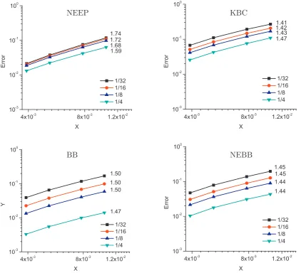
Wenowperformcommonconvergencetestsforaccuracy anal-ysis. Following the discussion inSection 2, we keep all parame-tersunchangedinphysicalunits.Wecheck theresultsata series ofcenterlinepointsadjacenttothewallboundary,namelyx=0.5 andy=1/32,1/16,1/8,1/4.AmoderateReynoldsnumberof400 isconsideredandthetopwallspeedissettobe0.1inthelattice

unit. Five sets ofgrids are investigated foreach boundary condi-tion,namely96×96,128× 128,192×192,256×256and512

× 512.The resultswiththefinestgridare consideredto be “cor-rect” to calculatethe actual simulationaccuracy, which isshown inFig.4.

Allthesimulationsshowsimilaraccuracy,althoughthoseusing the NEEP scheme show slightly higher accuracy. It is interesting toseethatthesimulationswiththeBBschemecanachieve accu-racy betterthan first-order.Thisreflects thefact thatthe conver-gencetestisactuallymeasuringtheaccuracyofsecondorderofEq. (5)(cf. Ref.[17],particularlyEq.(10) inPage 121.)oncethe non-physicalslipiscarefullyremovedfortheBBscheme,evenwithan on-grid implementation.Moreover, in comparisonwith theother three schemes, the first-order extrapolation of the NEEP scheme appearstoenhancethesimulationaccuracyinthebulkregion.

To study the numerical stability, we carry out two different tests. For the first test, we use a fixed number of grid pointsto simulatedifferentReynoldsnumber,andrecord themaximumRe thatcanbeachievedstably;Forthesecond,theReynoldsnumber is fixed with a difference number of grid pointsfor the simula-tions.Wethenrecordtheminimumgridpointnumberneededfor a stablesimulation. The results are listed inTables 3 and4. The KBC showsexcellent stability,which can be attributedto the fa-vorablepropertyofpositivity.TheNEEPschemealsohasgood sta-bilitywhiletheNEBBschemeisthelesssatisfactory.

The numerical efficiency of the boundary conditions is also measured by two criteria: the computational time needed for approaching the steady state determined by setting E=10−6 _in Eq.(17)andthecomputationaltimeforupdatingthewall bound-arypoints.Forthispurpose,werunsimulationsonanIntelCorei5 3.20GHZCPU.TheresultsforthefirstcriterionarelistedinTable5. Thereisnosignificantdifferencebetweenthefourschemes.Thisis particularlyinteresting for theKBC because previous simulations, usingadiscretevelocitymodel,becameincreasinglyslowerasthe Knudsennumberdecreased[15]forrarefiedgasflows.Ifwe con-siderthelatticeBoltzmannmodeltobeaspecialformofthe dis-cretevelocitymodel,theevidencehereshowsthatitpresents lit-tle differenceto thosespeciallydesignedboundaryconditionsfor continuumflows.

In Table 6, we list the computational time for updating all boundarypointsatthefourwallsduringonetimestep.Itisfound that theNEEP boundaryconditionneeds the longesttime, which is around 40 times more expensive than the most efficient BB scheme. This shows that the BB scheme should be an efficient choiceforsimulatingflowswithalargepercentageofsolid bound-arypoints,suchasparticle-fluidmultiphaseflows.

3.3. Stabilityforflowaroundasquarecylinder

Fig.2. Profilesofhorizontal(vertical)velocitycomponentthroughthevertical(horizontal)centerlineofcavityatRe=100(top),Re=400(middle)andRe=1000(bottom). Thehorizontalandverticalcomponents,uˆandvˆ,arenormalizedbythelidspeedUˆ,whichissettobe0.1forallthreecases.The‘NS’solutionsaretakenfromGhiaetal.

[30].

carefully setup flows so that critical

τ

ˆo _{valuesin the lattice unit} canbeachieved,i.e.,approaching0.5.

Aswithpriortests,westartfromapressure-drivenflow with-out theenclosedsquare cylinder.Thepressuredifferenceissetto be the0.00005(×

ρ

0RT0) andtheratio L/Dis setto be100. For this geometry,we test two sets ofReynolds numbers (calculated basedthemaximumspeedatthecenterline),0.0216and2.16,and thecorrespondingKnudsennumbersare0.0017and0.00017.With theseparameters, therelaxationtime

τ

ˆo _{inthelattice unit could} befairlysmallandapproachcriticalvalueforstabilityifthemesh iscoarse.Forinstance,using500×5cells,

τ

ˆo_{is0.5147and0.5015} receptively,seeEqs.(9)and(10)for the conversion.Wethen test thestabilityoffourwallboundaryschemesbyvaryingmeshsize. It isfound that theKBC andtheBB scheme allowstable simula-tions by using 500 × 5 cells for both Reynolds numbers, which

demonstratenicestability.FortheNEEPscheme,4000×40cells (

τ

ˆo_{=0.618) arerequiredforastablesimulationwithRe=0.0216} whilethecorrectsolutionisobtained.ForRe=2.16,wecannot ob-tainastablesimulationwithupto20000×200cells(

τ

ˆo_=0.559). This observation is generally consistent with previous findings. In[11], itis foundthat

τ

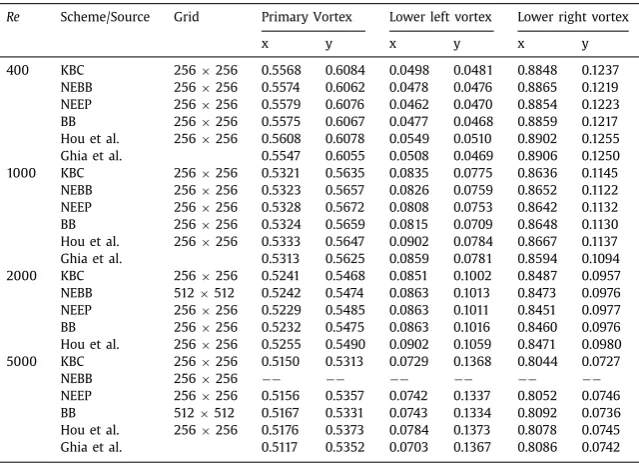
ˆo_{≈0.51is thethresholdifthe pressure} inlet/outletisalsoimplementedusingtheNEEPscheme,whilethe criticalvaluebecomesapproximately0.7ifextrapolationschemes areusedforbothwallandflowboundary.Therefore,theless satis-factorystabilitybehavioroftheNEEPschememaybeattributedto themixingwiththeextrapolationpressureflowboundary.Wealso notethattheNEEPschemeappearstoworkwellwithafixed ve-locityinletboundaryconditionforsimilarflowproblems[20].The NEBBschemealsofailstoachieveastablesimulationwith20000

[image:5.595.132.466.67.528.2]

Table2

Comparisonofvortexcenterlocations.Inallthepresentsimulations,thetop(north)wallspeedis0.1in latticeunits.ThebenchmarkresultsbyHouetal.aretakenfromtheLBsolutionslistedinTableIof[31]

andthoseofGhiaetal.arefrom[30].Usingthegrid256×256,theNEBBschemefailstomaintainstable simulationsforRe=5000.

Re Scheme/Source Grid PrimaryVortex Lowerleftvortex Lowerrightvortex

x y x y x y

400 KBC 256×256 0.5568 0.6084 0.0498 0.0481 0.8848 0.1237 NEBB 256×256 0.5574 0.6062 0.0478 0.0476 0.8865 0.1219 NEEP 256×256 0.5579 0.6076 0.0462 0.0470 0.8854 0.1223 BB 256×256 0.5575 0.6067 0.0477 0.0468 0.8859 0.1217 Houetal. 256×256 0.5608 0.6078 0.0549 0.0510 0.8902 0.1255 Ghiaetal. 0.5547 0.6055 0.0508 0.0469 0.8906 0.1250 1000 KBC 256×256 0.5321 0.5635 0.0835 0.0775 0.8636 0.1145 NEBB 256×256 0.5323 0.5657 0.0826 0.0759 0.8652 0.1122 NEEP 256×256 0.5328 0.5672 0.0808 0.0753 0.8642 0.1132 BB 256×256 0.5324 0.5659 0.0815 0.0709 0.8648 0.1130 Houetal. 256×256 0.5333 0.5647 0.0902 0.0784 0.8667 0.1137 Ghiaetal. 0.5313 0.5625 0.0859 0.0781 0.8594 0.1094 2000 KBC 256×256 0.5241 0.5468 0.0851 0.1002 0.8487 0.0957 NEBB 512×512 0.5242 0.5474 0.0863 0.1013 0.8473 0.0976 NEEP 256×256 0.5229 0.5485 0.0863 0.1011 0.8451 0.0977 BB 256×256 0.5232 0.5475 0.0863 0.1016 0.8460 0.0976 Houetal. 256×256 0.5255 0.5490 0.0902 0.1059 0.8471 0.0980 5000 KBC 256×256 0.5150 0.5313 0.0729 0.1368 0.8044 0.0727

NEBB 256×256 −− −− −− −− −− −−

NEEP 256×256 0.5156 0.5357 0.0742 0.1337 0.8052 0.0746 BB 512×512 0.5167 0.5331 0.0743 0.1334 0.8092 0.0736 Houetal. 256×256 0.5176 0.5373 0.0784 0.1373 0.8078 0.0745 Ghiaetal. 0.5117 0.5352 0.0703 0.1367 0.8086 0.0742

Fig.3. SlipvelocityinducedbytheKBCatthesouth(bottom)wallwithdifferent Reynoldsnumbers.Thetopwallspeedisfixedtobe0.1inlatticeunitssothat

ReisinverselyproportionaltoKnsinceKn×Re=Ma.Theslipvelocityisdefined asthedifferencebetweentheboundaryhorizontalvelocitygainedbycomputation andthatofthestationarywall.

Table3

MaximumReynoldsnumberachievedstablyusing afixednumberofgridpoints.FortheKBC,theRe

for512×512isnottestedsincethemaximumRe

isaround7500forlaminarflow.

Grid KBC NEBB NEEP BB

128×128 3000 400 1000 1000 256×256 7500 1000 5000 2000 512×512 −− 2000 7500 5000

Forthe flowaround asquare cylinder, wewill mainly investi-gatethestabilityoftheKBCandtheBB schemebasedonthe ob-servationofthepressure-drivenflow.Forthispurpose,thechannel lengthLissettobe15DandtheheightHequalto2.5Dwherethe flowwillfeeltheblockageeffects.Totestthestability,wesetupa casewith300 × 50cellsand

τ

ˆo_{=0.500866 (Kn=0.00001). The}

Table4

MinimumnumberofgridpointsneededforsimulatingafixedReynolds numberstably.For thecaseofRe=7500,only afew thousandtime stepsaretestedfortheBBandNEBBschemesduetothelargenumber ofgridpoints.

Re KBC NEBB NEEP BB

1000 96×96 256×256 96×96 96×96 2000 128×256 512×512 256×256 256×256 7500 256×256 2048×2048 512×512 2048×2048

Table5

Computationaltime(h)neededforapproachingthesteadystate deter-minedbysettingthecriterion,E=10−6_{,givenbyEq.(17).TheNEBB} schemeisnottestedforRe=5000sincethesimulationisnotstable.

Re Grid KBC NEBB NEEP BB

400 128×128 0.1038 0.1016 0.1010 0.1026 1000 256×256 1.2022 1.1025 1.3522 1.3540 2000 512×512 10.5536 10.2698 10.0537 10.3138 5000 512×512 33.0250 −− 33.5905 32.8989

Table6

Computational time (10−6 _{s) for updating boundary} points.

Re Grid KBC NEBB NEEP BB

1000 256×256 174 13.9 328 8.06

pressuredifferenceissettobe 10−8_(×

_ρ

0RT0). Bothschemescan achieve a stablesimulation,where“stable” means the simulation lasts at least 60000 iterations without the occurrence of “NAN” andafterwards we stop monitoring.Thisobservation further ver-ifiesthestabilityofboththeKBCandtheBBscheme.

[image:6.595.134.454.100.332.2] [image:6.595.48.283.121.515.2] [image:6.595.319.537.397.442.2] [image:6.595.321.535.494.548.2] [image:6.595.340.515.591.617.2] [image:6.595.85.235.619.663.2]

NEEP

KBC

BB

NEBB

Fig.4. Comparisonofnumericalaccuracyrelativetothenumericalsolutionusing512×512gridpointsatdifferentpointswithboundaryconditionsKBC,BB,NEBBand NEEP.Theaccuracyorder(slope)isshownbythefigurebesideeachline.TheReynoldsnumberissettobe400andthetopwallspeed0.1forallcalculations.

Fig.5. Streamlinesoftheflowaroundasquarecylindercapturedbysimulations usingtheBBscheme(top)andKBC(bottom).TheReynoldsnumberisestimatedto be28(seeSection3.3fordetailconfiguration).

Fig.5.TheReynoldsnumberisestimatedtobeabout28usingthe averagespeed atthe inlet.The simulationwiththeKBCproduces qualitativelysimilarresultstotheone withtheBBscheme,which againindicates that theslipvelocitywill playa minorroleifthe

Knudsen number is smalland the Reynolds number is sufficient large.

4. Concluding remarks

We have investigated the accuracy, stability, and efficiency of fourpopularboundaryconditionsforLBsimulation offlows with high Reynolds numbers. For the present study, the classical lid-drivencavityproblemistheprimarybenchmarkapplicationwhile thechannel flowaround asquare cylinderisused tosupplement theobservationofnumericalstability.

[image:7.595.94.517.58.442.2] [image:7.595.56.282.487.634.2]

wefindthatthecomputational timerequiredtoreach thesteady state for the lid-driven cavity flow is similar for all four bound-aryconditionsconsidered.Interestingly,theKBCscheme,whichis oftenused forrarefied gas flows, showsno significant difference in comparison to the other three boundary conditions specially designedforcontinuum flows. However, both the KBC andNEEP schemesneed asignificantly longertime toupdate theboundary pointswhilethe BBboundary condition,asexpected, isthemost computationallyefficient.

Acknowledgments

KNH and HWZ would like to thank the support of the Na-tional Key Research and Development Program of China under Grant No 2016YFB0200901. JPM and DRE would like to thank the Engineering and Physical Science Research Council (EPSRC) for their support under projects EP/L00030X/1, EP/N033841/1, EP/K038451/1 and EP/N016602/1. All authors from DL thanks by theHartreecenterfortheir support.YHZ wouldliketo thankthe supportofEPSRCundergrantnumberEP/M021475/1.

References

[1] ChenS,DoolenGD.LatticeBoltzmannmethodforfluidflows.AnnuRevFluid Mech1998;30(1):329–64.

[2] ShanX,ChenH.Simulationofnonidealgasesandliquid-gasphasetransitions bythelatticeBoltzmannequation.PhysRevE1994;49(4):2941.

[3] Wang M, Wang J, Pan N, Chen S. Mesoscopic predictions of the effec-tivethermalconductivityfor microscale randomporous media.PhysRevE 2007;75(3):036702.

[4] PengY,LiaoW,LuoL-S,WangL-P.ComparisonofthelatticeBoltzmannand pseudo-spectralmethodsfordecayingturbulence:low-orderstatistics.Comput Fluids2010;39(4):568–91.

[5] ChikatamarlaSS,FrouzakisCE,KarlinIV,TomboulidesAG,BoulouchosKB. Lat-ticeBoltzmannmethodfordirectnumericalsimulationofturbulentflows.J FluidMech2010;656:298–308.

[6] AidunCK,ClausenJR.Lattice-Boltzmannmethodforcomplexflows.AnnRev FluidMech2010;42(1):439–72.

[7] Jahanshaloo L, Sidik NAC, Fazeli A, A MPH. An overview ofboundary im-plementationinlatticeBoltzmannmethodforcomputationalheatandmass transfer.IntCommunHeatMass2016;78:1–12.

[8] Ladd AJC. Numerical simulations of particulate suspensions via a dis-cretized Boltzmann equation. Part 1. Theoretical foundation. J Fluid Mech 1994;271:285–309.

[9] ZouQ, HeX.Onpressureand velocityboundaryconditions for thelattice boltzmannBGKmodel.PhysFluids1997;9(6):1591–8.

[10] GuoZL,ZhengCG,ShiBC.Anextrapolationmethodforboundaryconditions inlatticeBoltzmannmethod.PhysFluids2002a;14(6):2007–10.

[11]GuoZL,ZhengCG,ShiBC.Non-equilibriumextrapolationmethodforvelocity andpressureboundaryconditionsinthelatticeBoltzmannmethod.ChinPhys 2002b;11(4):366–74.

[12] InamuroT,Yoshino M, OginoF. A nonâslipboundary condition for lattice Boltzmannsimulations.PhysFluids1995;7(12):2928.

[13]AnsumaliS,KarlinIV.KineticboundaryconditionsinthelatticeBoltzmann method.PhysRevE2002;66:026311.

[14]GatignolR.Kinetictheoryboundaryconditionsfordiscretevelocitygases.Phys Fluids1977;20(12):2022–30.

[15]ValougeorgisD,NarisS.Accelerationschemesofthediscretevelocitymethod: gaseousflowsinrectangularmicrochannels.JSciComput2003;25(2):534–52.

[16]Meng J, Zhang Y, Hadjiconstantinou NG, Radtke GA, Shan X. Lattice ellip-soidalstatisticalBGKmodelforthermalnon-equilibriumflows.JFluidMech 2013;718:347–70.

[17]HeX,ZouQ,LuoL-S,DemboM.Analyticsolutionsofsimpleflowsandanalysis ofnonslipboundaryconditionsfor thelatticeBoltzmannBGKmodel.JStat Phys1997;87:115–36.

[18]SuhYK,KangJ,KangS.Assessmentofalgorithmsfor theno-slipboundary conditioninthelatticeBoltzmannequationofBGKmodel.IntJNumer Meth-odsFluids2008;58(12):1353–78.

[19]MengJP,GuXJ,EmersonDR.SlipvelocityoflatticeBoltzmannsimulation us-ingbounce-backboundaryscheme.ArXive-prints.

[20]Nash RW, Carver HB, Bernabeu MO, Hetherington J, Groen D, Krüger T, etal.Choiceofboundaryconditionforlattice-Boltzmannsimulationof mod-erate-Reynolds-numberflowincomplexdomains.PhysRevE2014;89:023303.

[21]LattJ,ChopardB,MalaspinasO,DevilleM,MichlerA.Straightvelocity bound-ariesinthelatticeBoltzmannmethod.PhysRevE2008;77(5):56703.

[22]KaoP-H,YangR-J.Aninvestigationintocurvedandmovingboundary treat-mentsinthelatticeboltzmannmethod.JComputPhys2008;227(11):5671–90.

[23]ShanXW,YuanXF,ChenHD.Kinetictheoryrepresentationofhydrodynamics: awaybeyondtheNavierStokesequation.JFluidMech2006;550:413–41.

[24]ShanX,HeX.Discretizationofthevelocityspaceinthesolutionofthe Boltz-mannequation.PhysRevLett1998;80:65–8.

[25]HeX,LuoL-S.TheoryofthelatticeBoltzmannmethod:fromtheBoltzmann equationtothelatticeBoltzmannequation.PhysRevE1997;56:6811–17.

[26]MengJ,ZhangY.Accuracyanalysisofhigh-orderlatticeBoltzmannmodelsfor rarefiedgasflows.JComputPhys2011;230(3):835–49.

[27]HeX,ChenS,Doolen GD.AnovelthermalmodelforthelatticeBoltzmann methodinincompressiblelimit.JComputPhys1998;146(1):282–300.

[28]Meng J,Zhang Y. Diffuse reflectionboundary condition for high-order lat-ticeBoltzmannmodelswith streaming-collisionmechanism.J ComputPhys 2014;258(0):601–12.

[29]GuoZ,ShuC.LatticeBoltzmannmethodanditsapplicationsinengineering. vol.3advancesincomputationalfluiddynamicsWorldScientific;2013. [30]Ghia U, Ghia KN, Shin C. High-re solutions for incompressible flow

us-ing the Navier–Stokes equations and a multigrid method. J Comput Phys 1982;48(3):387–411.

[31] HouS,ZouQ,ChenS,DoolenG,CogleyAC.Simulationofcavityflowbythe latticeBoltzmannmethod.JComputPhys1995;118(2):329–47.