Strongly polynomial primal monotonic build-up simplex algorithm for maximal
ow problems
Tibor Illésa, Richárd Molnár-Szipaib
aBudapest University of Technology and Economics, [email protected]
bBudapest University of Technology and Economics, [email protected], corresponding author
Abstract: The maximum ow problem (MFP) is a fundamental model in operations research. The network simplex algorithm is one of the most ecient solution methods for MFP in practice. The theoretical properties of established pivot algorithms for MFP are less understood. Variants of the primal simplex and dual simplex methods for MFP have been proven strongly polynomial, but no similar result exists for other pivot algorithms like the monotonic build-up or the criss-cross simplex algorithm.
The monotonic build-up simplex algorithm (MBU SA) starts with a feasible solution, and xes the dual feasibility one variable at a time, temporarily losing primal feasibility. In the case of maximum ow problems, pivots in one such iteration are all dual degenerate, bar the last one. Using a labelling technique to break these ties we show a variant that solves the maximum ow problem in2|V||E|2pivots.
Keywords: maximum ow problem; pivot algorithm; MBU algorithm
1. Introduction
The maximal ow problem is one of the basic models in network optimization that has a wide range of applications (see e.g. [1]). It is not surprising then, that it has been studied extensively, with numerous solution methods developed.
The rst substantial results are due to Ford and Fulkerson [8], including the maximum ow minimum cut theorem, and the idea of augmenting path algorithms. Later Edmonds and Karp [7], and independently Dinic [6] proved that the shortest augmenting path algorithm is strongly polynomial.
Another family of algorithms use so-called preows. A preow is a ow except that each intermediate node are allowed to have more inow than outow (but not the other way around). The rst such algorithm by Karzanov [14] used preows only to solve the subproblems in Dinic's algorithm, so the conservation equations are restored at the end of each phase. Later preow algorithms took a more holistic approach, where the preow becomes a ow only at the nal step (see e.g. Goldberg and Tarjan [9]). This phenomenon is similar to how primal feasibility is restored only at the last pivot of a dual simplex algorithm, while the augmenting path algorithms are more like the primal simplex algorithm in that they proceed through feasible solutions.
In fact, the maximum ow problem is a special linear programming problem, therefore it can be solved using pivot algorithms. Indeed, the description of the network simplex algorithm appears as far back as Dantzig's book on linear programming [5]. The rst published strongly polynomial pivot algorithm for a network optimization problem is a dual simplex algorithm for the minimum cost ow problem due to Orlin [15], while the rst primal simplex variant, specically for the maximum ow problem, is by Goldfarb and Hao [10, 11]. Later Orlin showed that a strongly polynomial variant of the primal simplex algorithm for minimum cost ow problems also exists [16]. Pivot algorithms that traverse bases that are neither primal nor dual feasible, however, received less attention, no such algorithm has been proven strongly polynomial so far. We show that the primal monotonic build-up simplex algorithm [2] has a strongly polynomial variant for the maximum ow problem.
A further generalisation of the preow concept was given by Hochbaum [12], where the so-called pseudoow can have unbalanced intermediate nodes even with the outow being greater than the inow. The algorithm solves the maximum blocking cut problem rst, which provides a minimum cut, and then recovers a maximum ow. After each iteration a feasible ow could be recovered using a process analogous to ow decomposition, giving the algorithm a primal character. In fact, Section 10 describes a simplex variant of the algorithm.
solution, and use a suitable pivot algorithm to reach a feasible basic solution. One such pivot algorithm is the feasibility MBU SA, which can be thought of as a dual MBU SA with the objective function of constant zero. The authors showed that the feasibility MBU SA has a variant that nds a feasible basic solution in strongly polynomial time in [13].
The structure of the article is as follows: in the next section we describe the MBU SA for linear programming in general and how it works on maximum ow problems in particular, then we describe our variant in detail. In the third section we describe the generic pseudoow algorithm [12], place it in a pivot framework and compare it with the MBU SA. In the fourth section we prove the polynomiality of our MBU SA variant, and then conclude the article with some remarks and possible future research directions.
2. Preliminaries
The reader is expected to have a basic understanding of the simplex method of linear programming (e.g. basic solutions, primal and dual feasibility), and of the maximum ow problem. For reference, see [1, 5, 8].
Consider a linear programming problem in the following form:
maxcTx
Ax=b x≥0
Where A∈ Rn×m, x,c ∈Rm, b∈ Rn. Without loss of generality we may assume thatA has full row rank. LetB be ann×ninvertible submatrix ofA,IB the set of column indices of B, andIN the remaining column
indices. Then the solution xB =B−1b, xN =0is a so-called basic solution, with the corresponding simplex
tableau:
A b cT −z0
:= B
−1A B−1b
cT −cT
BB−1A −cTBB−1b
Using the notationsai,j,biandcj for the elements of the current tableau, the primal MBU SA is as follows:
1. Start with a primal feasible basic solution
2. Choose a dual infeasible variable xp∗. We refer toxp∗ as the driving variable [2]. If there are none, stop,
we have an optimal solution.
3. Select the leaving variable using a minimum ratio test on feasible basic variables:
q= arg min
b
q
aq,p∗
: aq,p∗>0, bq ≥0
Letϑ1=|cp∗|/aq,p∗.
4. Choose the entering variable using a minimum ratio test on dual feasible nonbasic variables:
p= arg min
c
p
|aq,p| : cp≥0, aq,p<0
Letϑ2=cp/|aq,p|.
5. Variable xq leaves the basis. If ϑ2 < ϑ1, thenxp enters the basis and go to step 3, otherwise xp∗ enters
the basis, and go to step 2.
The name of the algorithm comes from the property that dual feasible variables do not lose their feasibility (due to step 4), and thus the set of these variables monotonically build up. The fact that we might select the variable xp instead of xp∗ on whose column we took the minimum ratio test means that we can lose primal
feasibility. However, whenxp∗ nally enters the basis, primal feasibility is restored (see [2] for details).
maxxt,s
∀v∈V : X (w,v)∈E
xw,v−
X
(v,w)∈E
xv,w= 0
∀e∈E: le≤xe≤ue
Throughout the article we are using the following notations:
• v,wandz for nodes of a graph
• efor an arc of a graph
• pandqfor the entering and leaving arc of a graph
• p∗= (g, h)as the arc corresponding to the driving variable
Now let us break down how the primal monotonic build-up simplex algorithm works on maximum ow problems step by step.
Step 1 : Start from a primal feasible basic solution. The basic variables correspond to the arcs of a spanning treeT containing(t, s), with the nonbasic arcs having ow values of either the lower or the upper bound. The
basic variables are then uniquely determined by the conservation equations. If the lower bounds are zero, then
x = 0 is such a feasible basic solution with an arbitrary spanning tree. Otherwise nding such a starting
solution is not trivial, one can do so by transforming the network and solving another (zero lower bounds) maximum ow problem (see e.g. [1] section 6.2), which corresponds to solving the rst phase of a two phase linear programming problem. Another way is to use the feasibility MBU SA [13] (which is a specialization of [4]). Having zero or nonzero lower bounds do not aect the algorithm otherwise.
Step 2 : Choose a dual infeasible variablexe. LetTi ⊂Ebe the spanning tree before theith pivot. Dropping (t, s)fromTidisconnects the spanning tree, with one subset containings, and the other one containingt. These vertex sets are denoted bySi andZi respectively. The reduced costc
eof a nonbasic arceis:
ce=
1 ife:Si→Zi andx
e=ueor e:Zi →Si andxe=le −1 ife:Si→Zi andx
e=leor e:Zi→Si andxe=ue 0 otherwise: e:Si→Si ore:Zi→Zi
Without loss of generality we can assume that the driving variable p∗ = (g, h)∈E is on its lower bound, i.e. g∈Si andh∈Zi.
Step 3 : Choose the leaving variable with a primal ratio test. Ti∪(g, h)contains a unique cycleCi, consider
it directed according to(g, h). Then the leaving arcq∈Ci is an arc where
δ= min
uq−xq: q is forward,xq ≤uq; or
xq−lq : q is backward,xq ≥lq
takes its value. (We are examining how much we could augment along the cycleCi, not counting arcs that are
already infeasible in the appropriate direction.) Note that such an arcq is uniquely determined if the bounds are suciently diverse, so we will choose arbitrarily, should a tie occur.
Step 4 : Choose the entering variable with a dual minimum ratio test. The simplex tableau, along with the reduced costs is totally unimodular, so this ratio test can result in either a 0, or a 1 quotient. As ϑ1= 1 the
only instance when we do not letp∗ enter the basis is if we nd an arc pwith ratio 0, i.e. with reduced cost 0, andaq,p=−1. As we've seen, cp = 0means thatpis eitherSi →Si or Zi →Zi, andϑ2< ϑ1means that
performing the pivot(g, h)forqwould makepdual infeasible. In the case ofq∈Si, dropping q from the tree
would disconnectsandg, suitable entering variables would either be arcs from the subtree ofsto the subtree ofg on their lower bounds, or arcs the other way around on their upper bounds.
The general properties of the MBU SA carry over to this more special problem, that is no dual feasible variable ever becomes dual infeasible, and while primal feasibility can be temporarily lost during the phase of a driving variable, it is restored at the end of such a phase when the driving variable enters the basis.
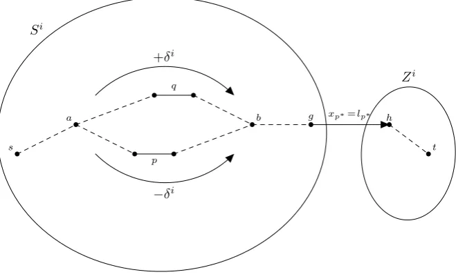
Lemma 1. Assume that a MFP is solved by the MBU SA,p∗= (g, h)is the current driving variable withg∈S andh∈Z. Then the following statements hold for all pivot index i≥0, whilep∗ does not enter the basis (δ0 is interpreted as0):
a) all primal infeasible arcs after theith pivot are on the s→g and the h→t paths,
b) the arcs in the direction of the paths can only violate their lower bound, the backward arcs only their upper bounds, both by at most δi,
c) the next pivot will haveδi+1≥δi.
When p∗ enters the basis, primal feasibility is restored.
Proof: For i= 0 the statements hold, as there are no primal infeasible arcs before the rst pivot, δ0= 0,
andδ1≥0will be true by denition.
For i ≥ 1 we use induction. Assume that the lemma holds for the pivots up to i−1. Without loss of
generality we might assume that the leaving arc q, and therefore the entering arc ptoo, is in S. The cycle resulting from addingphas a common segment with thes→g path (containingq), let us denote its endpoints by a andb, see Figure 1. After the pivot this a →b segment will be replaced by the other half of the cycle (containing p) in the s→g path. The ow value on the olda→b segment (containingq) is increased by δi,
the ow value on the newa→bsegment (containingp) is decreased byδi.
Si
Zi
s
a
q
b
p
g xp∗=lp∗ h
t +δi
[image:4.595.134.464.323.525.2]−δi
Figure 1: The structure of pivoti.
According to the induction hypothesis, the primal infeasible arcs before pivotiare on thes→g path, with infeasibility at mostδi−1 andδi≥δi−1. Therefore increasing the ow value on the olda→bsegment restores
the primal feasibility of those arcs, and so statement a) holds.
The arcs on the new a→b segment were feasible before pivoti by the induction hypothesis, and the ow value was decreased byδi on the segment. This way the arcs in thea→b direction (which is the same as the
direction of the news→gpath) could go below their lower bounds by at mostδi, and the arcs in the opposite
direction can surpass their upper bounds by at mostδi. Thus statement b) holds.
Finally, as the arcs on the new a→b segment were decreased byδi from a feasible position, they can be increased by at least that much in the next pivot. The ow values of the arcs on thes→a,b→gand h→t paths were not changed, but they could have been increased by at leastδi by the calculation ofδ before pivot i. Therefore after the pivot all arcs on the news→g andh→t paths can be increased by at least δi, and so
δi+1 ≥δi will hold too.
Ifp∗ enters the basis in thek+ 1st pivot, then the previous statements hold for pivotk: the infeasible arcs are all on thes→gandh→tpaths, their infeasibility is at mostδk, their direction is such that increasing the
ow along the paths decrease their infeasibility, and due toδk+1≥δk thek+ 1st pivot will make them feasible
Note that by the above lemma primal feasibility can be restored at any pivot by letting the driving variable enter the basis, however, new dual infeasible arcs appear if there were candidates forp. This is consistent with the behaviour of the primal MBU SA on linear programming problems.
To describe our variant we will consider the subtreesSiandZito be rooted atgandhrespectively. Picturing the tree with the root at the top, and using the usual notions of parent and child node,Tvi will denote the
subtree in Ti spanning the node v and its descendants. Using this image, we will also refer to the nodes of a
basic arc as the upper and lower nodes. For a basic arcq∈Ti we will use the notationTi
q for the subtree
below q, that is,Ti
v, wherevis the lower node ofq(we will use this notation only in the context of the leaving
variableq).
We will use the concept of a pseudo-augmenting path (PAP) as dened in [11]: a pseudo-augmenting path from v to w with respect to a basic solution x, and spanning treeTi is a directed path from v to w that can use(v1, v2)if
• (v1, v2)∈E\Ti andxv1,v2 =lv1,v2,
• or (v2, v1)∈E\Ti andxv2,v1 =uv2,v1,
• or if either (v1, v2)∈Ti or(v2, v1)∈Ti.
Note that nonbasic arcs are used the same way as with classical augmenting path algorithms, the addition of using basic arcs in any direction makes the notion compatible with the basis structure.
The label di(v)of vertexvbefore pivotiwith respect to the current driving variable(g, h)and basis structure
Ti is the length of the shortest PAP fromhtov withinTi
h ifv∈Thi, and the length of the shortest PAP from
v tog withinTi
g ifv∈Tgi.
Using these labels to choose the entering variable results in the following variant of the primal monotonic build-up simplex algorithm:
Algorithm 1 Primal monotonic build-up simplex algorithm with labelling Start with a primal feasible basic solutionx.
whilexis not optimal do
Letp∗= (g, h)be an arbitrary dual infeasible arc.
whilep∗ is dual infeasible do
Letqbe an arc limiting further augmentation along the cycle inTi∪(g, h).
if there is a possible entering arc betweenTqiand the rest ofTgi or Thi (whicheverqis in) then
Letpbe such an arc with minimal label inE\Ti q.
Perform a pivot withpentering andqleaving the basis. else
Perform a pivot withp∗entering the basis and qleaving. end if
end while end while
3. Comparison with the pseudoow algorithm of Hochbaum
Let us rst extend our network. Recall that G= (V, E)is a directed graph with source s and sink t, to which we added an arc (t, s). For each node v, two arcs of innite capacity (and 0 lower bound) are added: (t, v)and(v, s). These arcs are referred to as decit arcs and excess arcs respectively. Finally, the nodessand tare shrunk into a single noder, referred to as the root. This extended network will be denoted byGEXT.
The pseudoow algorithm aims to maximize the ow value, while maintaining a pseudoow at every step, that is ow values that satisfy the capacity constraints, but might violate the ow balance constraints. Such a pseudoow has a corresponding feasible ow on the graph GEXT, as a node v with decit can be balanced by letting ow in via the(r, v)arc, and excess can be drained using the excess arc(v, r).
The pseudoow algorithm maintains a construction called a normalized tree, which is a spanning treeT in GEXT with rootr. The children of rare denoted byri and called the roots of their respective branches. Then
1. all arcs(s, v)and(v, t)in the original network are saturated (xe=ue for suchearcs),
2. xis equal to the lower or upper bounds on out-of-tree arcs.
3. In every branch, all downwards residual capacities are strictly positive.
4. Only the rootsri might not satisfy ow balance constraints in the original network.
Note that property 4 is a consequence of property 2, as an unbalanced nodev must have positive ow value on either its decit or excess arc, which arc (due to property 2) must be inT, and thusv is a neighbor ofrin the tree.
To describe the algorithm we introduce further notions. A branch of the current normalized treeT is called strong, if its root ri has positive excess, and is called weak otherwise (including the case that ri is balanced).
The collection of strong branches will be denoted byS, the weak branches byW. Also, we denote the excess of a nodevin the original network bye(v)(the sum of incoming ow minus the sum of outgoing ow).
The algorithm starts with an initial normalized tree and pseudoow, and looks for arcs between S and W with residual capacity towardsW. After pushing ow from the root of the strong branch towards the root of the weak branch, a restructuring is performed to maintain the normalized tree structure.
Algorithm 2 Generic pseudoow algorithm
LetT be an initial normalized tree with initial pseudoowx.
while there are arcs with residual capacity in(S, W)do
Select(s0, w)∈(S, W)with residual capacity.
Letrs0 andrwbe the roots of the branches containing s0 andwrespectively.
Letδ=e(rs0) =xr
s0,r.
Merge{(s0, w)}:
LetT =T ∪(s0, w)\(rs0, r).
Letxrs0,r= 0.
Renormalize:
Let(v1, . . . , vk) = (rs0, . . . , s0, w, . . . , rw, r).
Leti= 1.
repeat
if the residual capacitycr
vi,vi+1 of(vi, vi+1)is at leastδthen
Augment ow on(vi, vi+1)byδ
else
Split{(vi, vi+1), δ−crvi,vi+1}:
LetT =T∪(vi, r)\(vi, vi+1).
Letxvi,r =δ−c r vi,vi+1.
Letδ=cr vi,vi+1.
Augment(vi, vi+1)byδ.
end if Leti=i+ 1
untilvi+1=r
end while
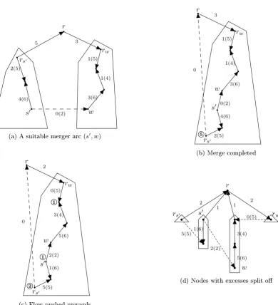
The algorithm can be easier understood through an example. In Figure 2 we can follow an iteration of the algorithm. The numbers on arcs show the current ow value, with the upper bound in parentheses (lower bounds are zero), while the encircled numbers show the excess of a node. Subgure 2a shows a suitable arc
(s0, w)from a strong branch to a weak branch with residual capacity. Subgure 2b shows the merging of the
two branches, withxrs0,r = 0, and5 excess at rs0. In Subgure 2c we pushed as much ow from rs0 upwards
as the bounds allowed, creating nodes with positive excesses. Subgure 2d shows how the splitting procedure turns nodes with positive excesses into roots of new strong branches.
When the algorithm terminates, the cut between the strong and weak branches can be showed to be a minimum cut, and a maximum ow can be recovered using a procedure based on ow decomposition (see [12] section 8).
The algorithm is very similar to a pivot algorithm, as the pseudoow after every iteration can be turned into a basic feasible ow, using the procedure mentioned above. These basic solutions are, however, not neighboring in the sense that getting from one such basic solution to the next one is not possible with a single pivot.
In fact, there is a simplex variant described in [12] section 10, that after the merging operation calculates the minimum residual capacity along the[rs0, . . . , s0, w, . . . , rw, r]path, pushes only this much upwards, and lets
r
rs0
rw
s0 w
5 3
2(5)
4(6)
0(2)
3(6) 1(4) 1(5)
(a) A suitable merger arc(s0, w)
r
rs0
rw
s0 w
5
3
2(5) 4(6) 0(2)
3(6) 1(4) 1(5)
0
(b) Merge completed r
rs0
rw
s0 w
2
2
5(5) 1(6)
1 2(2)
5(6) 3(4)
1
0(5)
0
(c) Flow pushed upwards
r
rs0 s0 rw
w
2
1 1
2
1(6)
5(6) 3(4) 5(5)
2(2)
0(5)
[image:7.595.100.491.62.491.2](d) Nodes with excesses split o
Figure 2: An iteration of the pseudoow algorithm
However, Algorithm 2 can be also described as a pivot algorithm, where a single iteration consists of multiple pivots: one pivot for the merge operation, and one pivot for each split operation. The Merge{(s0, w)} operation
has (s0, w) entering and (rs0, r) leaving the basis with the whole δ = e(rs0) =xr
s0,r ow pushed around the
cycle, making some basic arcs infeasible. Then the split operations recover a feasible ow by taking the rst infeasible arc(vi, vi+1)on the path, making it leave the basis with(vi, r)entering, and the infeasibility pushed
back around this cycle, and repeating this process until no infeasible arcs remain.
This way Algorithm 2 is also a pivot algorithm traversing bases that are neither primal nor dual feasible. The entering arc is dual infeasible, but the leaving arc is not chosen according to a primal ratio test, therefore primal feasibility is lost. Then a structured sequence of pivots making primal infeasible arcs leave the basis, and the articial(vi, r)arcs entering it restores feasibility. The advantage of this method is that a larger augmentation
can be performed in the merger pivot than with the ratio test.
Comparatively, Algorithm 1 chooses a dual infeasible variable, but does not let it enter until it is safe to do so, in the sense that no new dual infeasible arcs are created. The price of this safety is that the pivots leading up to the driving variable nally entering the basis are dual degenerate, and so the objective function stagnates in the meantime.
4. Proving Strong Polynomiality
First, we need to note that it is sucient to establish the polynomiality of making a single (g, h) dual
variable never becomes infeasible during the algorithm, and so the number of outer cycles is bounded by the number of dual infeasible variables in the initial basic solution.
To bound the number of pivots needed to get the driving variable into the basis, we use a few features of the labelling technique. First, we prove that the label of every node is monotonically non-decreasing (monotonicity lemma). This tells us that the algorithm is progressing in a certain sense. The lemma's appropriate version appears in the proofs of polynomiality for both the primal and the dual simplex variant ([11] and [3]).
As the label of a node represents the length of a shortest path, it is bounded by the number of vertices. After the monotonicity lemma we show that not only the labels do not decrease, but strict increases must happen regularly. Thus we will be able to derive an upper bound on the number of pivots.
The structure is based on Lemma 3. of [3]. We show in Lemma 5 (main lemma) that for every arc p = (pv, pw) the sum of its labels d(pv) +d(pw) must increase between subsequent enterings into the basis.
This is split into two cases according to whetherpleaves the basis having the same direction that it had when entering or not, their proofs aided by Lemmas 3 and 4 respectively. Due toSi andZi not behaving like a dual
feasible basis in [3], these lemmas are somewhat weaker, and their proofs somewhat more convoluted.
Lemma 2 (Monotonicity lemma). Assume that a MFP is solved by Algorithm 1. For any v ∈ V and iteration iduring a single outer cycledi+1(v)≥di(v)holds.
Proof: Assume indirectly that there exists z and i such that di+1(z) < di(z). We can assume thatz is a
counterexample with minimaldi+1(z)label.
Asdi+1(z)< di(z), the shortest PAP fromztogafter theith pivot must use an arc in a direction that was
not available before. Let us take a look at how the arcs change with respect to labelling:
• arcs that are in the basis both before and after the pivot (Tgi∩Tgi+1) can be used in both directions for calculatingdi(z)anddi+1(z),
• arcs not in either basis (E\(Ti
g∪Tgi+1)) didn't have their ow value changed, so they can be used in the
same directions both before and after the pivot,
• the entering arc pwas usable in one direction before entering the basis, and is usable in both directions after the pivot,
• conversely, the leaving arcqwas usable in both directions before the pivot, and in only one direction after it.
Letv∈Ti
q andw6∈Tqi be the two vertices ofp, the only new possibility for labelling after the pivot is using
pin thew→v direction, so the new shortest PAP fromz must use that.
As v∈Tqi, this PAP must leaveTqi after usingpvia somep0 arc, withv0∈Tqi and w06∈Tqi its two vertices. Note thatp06=q, because after leaving the basisqcan only be used from its vertex not inTi
q. Thereforep0 6∈Ti,
and could have been used to leave Ti
q, so it was a candidate for entering the basis at theith pivot. However,
we chosepoverp0, sodi(w)≤di(w0)must hold.
Therefore the shortest PAP fromztogrst uses the shortest PAP fromztow, uses(w, v), uses the shortest
PAP fromv tov0, uses(v0, w0), and nally the shortest PAP fromw0 to z. Denoting the shortest PAP fromv1
tov2before pivotk bydk(v1, v2),di+1(z)can be written as:
di+1(z) =di+1(z, w) + 1 +di+1(v, v0) + 1 +di+1(w0)
≥di(z, w) +di(w0) + 2≥di(z, w) +di(w) + 2≥di(z) + 2.
Where we used:
• di+1(z, w)≥di(w, z), as the shortest PAP fromz towcan not usepin thew→v direction.
• di+1(v0, v)≥0.
• di+1(w0) ≥di(w0), as otherwise w0 would be a counterexample to the lemma, with di+1(w0)< di+1(z),
contradicting the minimality of z.
• di(w) +di(w, z)≥di(z)is a triangle inequality for PAPs.
We assumed indirectly thatdi+1(z)< di(z), but we concluded di+1(z)≥di(z) + 2, a contradiction.
To proceed, we will prove an inequality that will help us in both cases of the main lemma.
Lemma 3 (Subtree lemma). Assume that a MFP is solved by Algorithm 1. If(v, w)entered the basis at the
ith pivot, with wbeing the upper vertex, and this remains true throughout, even after the jth pivot, then for all z∈Tj+1
v : dj+1(z)≥di(w) + 1.
Proof: Case j=i. Note thatTi+1
v =Tqi. Take a shortest reverse pseudo-augmenting path fromg to z. As
z∈Ti+1
v , this path must contain an arc leading intoTqi. This arc can not beq, as it left the basis on the wrong
bound for that.
If it isp, thendi+1(z)≥di+1(w) + 1≥di(w) + 1.
Otherwise that arc could have entered the basis at pivoti, but we chosepinstead, sodi(w0)≥di(w)for its
w06∈Tqi vertex. Thendi+1(z)≥di+1(w0) + 1≥di(w0) + 1≥di(w) + 1.
This nishes the proof for j=i.
Forj > iwe use induction, so let us assume that the lemma is true forj−1, and letz∈Tj+1
v .
Ifz∈Tj
v as well, then monotonicity and the induction hypothesis givesdj+1(z)≥dj(z)≥di(w) + 1.
Otherwise, z entered Tv during the jth pivot. Let the entering arc of that pivot bep with pv ∈ Tvj and
pw6∈Tvj vertices. Thendj+1(z)≥dj(pv) + 1using thei=j case of this lemma forp, anddj(pv)≥di(w) + 1
by the induction hypothesis, givingdj+1(z)≥di(w) + 2. This completes the proof.
The next lemma shows that ifpchanges direction since entering the basis, then a strict increase in his labels must already have happened.
Lemma 4 (Reversal lemma). Assume that a MFP is solved by Algorithm 1. If (v, w) entered the basis at
the ith pivot, with w being the upper vertex, this remains true throughout, but changes tov being upside with the jth pivot, then dj+1(w)≥di(w) + 1.
Proof: We claim that the following inequalities hold:
dj+1(w)≥dj(pw) + 1≥dj(pv)≥di(w) + 1
Let the entering arc at pivotj bepwith pw 6∈Tvj andpv ∈Tvj vertices. The leaving arcq must be on the
path in the spanning tree fromw to g for(v, w)to change directions. This also means that w∈Tj+1 pw , so by
the subtree lemma we havedj+1(w)≥dj(pw) + 1.
As p was a candidate for entering, it could be used for labelling from thepw end, which means dj(pv)≤
dj(p w) + 1.
Finally,pv∈Tvj, so using the subtree lemma we getdj(pv)≥di(w) + 1.
Now we are ready to state our main lemma, describing the growth behavior of the labels.
Lemma 5 (Main lemma). Assume that a MFP is solved by Algorithm 1. If (v, w) entered the basis at pivot
i, left it at pivot j, and entered it again at pivotj, thendk+1(v) +dk+1(w)≥di(v) +di(w) + 2holds.
Proof: Without loss of generality we might assume that wis the upper vertex of(v, w)inTi+1
g .
Case a: wis the upper vertex inTgj as well. We claim that
dk+1(v) +dk+1(w)≥2dk(v) + 1≥2di+1(v) + 1≥di(v) +di(w) + 2
After leaving a base(v, w)can be used for labelling only from itsv end, thereforevwill be the upper vertex after pivotk. According to the subtree lemma dk+1(w)≥dk(v) + 1, and usingdk+1(v)≥dk(v)we get the rst
inequality.
The second inequality is the monotonicity lemma.
In the third inequality we bound one of the di+1(v)with the subtree lemma: di+1(v)≥di(w) + 1, and the
other one with monotonicity: di+1(v)≥di(v).
Case b: vis the upper vertex in Tj
g. We explain
wherel is the rst pivot when the direction of(v, w)changes in the spanning tree (i < l < j < k).
As v is the upper vertex when leaving the basis, w is the upper vertex after pivot k, and we get the rst inequality by using the subtree lemma and monotonicity similar to the previous case.
The second inequality is the monotonicity lemma.
The third inequality is the reversal lemma: dl+1(w)≥di(w) + 1.
In the fourth inequality we use that before pivot i we could use (v, w) for labelling from the side of w, thereforedi(v)≤di(w) + 1.
Finally, we deduce the strong polinomiality of the algorithm from the previous lemma.
Theorem 1. Algorithm 1 solves a MFP in at most 2nm2 pivots.
Proof: The number of dual infeasible arcs at the start of the algorithm is less thanm. As the primal MBU simplex algorithm does not create new dual infeasible arcs, the inner cycle can happen at mostm times. Let us then examine the number of pivots it takes to x an infeasible arc.
For any(v, w)arc we have1≤d(v) +d(w)≤2n−5(we have 2 vertices with label0, so the maximum label
isn−2, and there can be at most one such vertex). By the monotonicity lemmad(v) +d(w)is not decreasing,
and by the previous lemma it increases by at least 2 if it enters the basis twice. Therefore(v, w)can enter the
basis at most 2n−5 times. As every pivot has an entering arc, we can thus have at most 2nmpivots, even counting the nal pivot that lets the dual infeasible arc enter the basis.
5. Conclusions and further directions
Building upon the techniques used for proving the polynomiality of certain variants of the primal and dual simplex algorithms [11, 3] on the maximum ow problem, we have shown that the primal MBU SA also has such a strongly polynomial variant. This variant has an interesting structure: the algorithm makes at mostm dual nondegenerate steps, each two separated by at most 2nmdual degenerate steps. The corresponding ow becomes primal feasible after every nondegenerate step, but this property may not hold in between them.
It remains an open problem if similar results can be reached with other non-primal, non-dual pivot algorithms, such as the dual MBU SA, exterior point simplex algorithms [17], or criss-cross type algorithms [18]. Another interesting question is whether the results can be generalized to minimum cost ow problems.
Acknowledgements.We are grateful for the work of the two anonymous reviewers, and also for the sug-gestion of including lemma 1 in the article.
Tibor Illés acknowledges the research support obtained from Strathclyde University, Glasgow under the John Anderson Research Leadership Program.
References
[1] R. K. Ahuja, T. L. Magnanti, and J. B. Orlin. Network Flows. Prentice Hall, New Jersey, 1993.
[2] K. M. Anstreicher and T. Terlaky. A monotonic build-up simplex algorithm for linear programming. Operations Research, 42:556561, 1994.
[3] R. D. Armstrong, W. Chen, D. Goldfarb, and Z. Jin. Strongly polynomial dual simplex methods for the maximum ow problem. Mathematical Programming, 80:1733, 1998.
[4] F. Bilen, Zs. Csizmadia, and T. Illés. AnstreicherTerlaky type monotonic simplex algorithms for linear feasibility problems. Optimisation Methods and Software, 22(4):679695, 2007.
[5] G. B. Dantzig. Linear Programming and Extensions. Princeton University Press, Princeton, NJ., 1963. [6] E. A. Dinic. Algorithm for solution of a problem of maximum ow in networks with power estimation.
Soviet Math. Doklady, (11):12771280, 1970.
[7] J. Edmonds and R. M. Karp. Theoretical improvements in algorithmic eciency for network ow problems. Journal of ACM, 19:248264, 1972.
[8] L. R. Ford and D. R. Fulkerson. Flows in Networks. Princeton University Press, Princeton, NJ., 1962. [9] A. V. Goldberg and R. E. Tarjan. A new approach to the maximum ow problem. In Proceedings of the
[10] D. Goldfarb and J. Hao. A primal simplex algorithm that solves the maximum ow problem in at most nmpivots andO(n2m)time. Mathematical Programming, 47:353365, 1990.
[11] D. Goldfarb and J. Hao. On strongly polynomial variants of the network simplex algorithm for the maximum ow problem. Operations Research Letters, 10:383387, 1991.
[12] D. S. Hochbaum. The pseudoow algorithm: A new algorithm for the maximum-ow problem. Operations Research, 56(4):9921009, 2008.
[13] T. Illés and R. Molnár-Szipai. On strongly polynomial variants of the MBU-simplex algorithm for a maximum ow problem with non-zero lower bounds. Optimization, 63:3947, 2014.
[14] A. V. Karzanov. Nakhozhdenie maksimal'nogo potoka v seti metodom predpotokov (determining the maximal ow in a network by the method of preows). Doklady Akademii Nauk SSSR, 215(1):4952, 1974.
[15] J. B. Orlin. Genuinely polynomial simplex and non-simplex algorithms for the minimum cost ow problem. Technical report, Technical Report 1615-84, Sloan School of Management, MIT, Cambridge, MA., 1984. [16] J. B. Orlin. A polynomial time primal network simplex algorithm for minimum cost ows. Mathematical
Programming, 78:109129, 1997.
[17] K. Paparizzos, N. Samaras, and A. Sifaleras. Exterior point simplex-type algorithms for linear and network optimization problems. Annals of Operations Research, 229(1):607633, 2015.