Equilibrium Investment in High Frequency Trading Technology: A Real Options Approach

      

City, University of London Institutional Repository

Citation

:

Delaney, L. (2016). Equilibrium Investment in High Frequency Trading

Technology: A Real Options Approach (15/14). London, UK: Department of Economics, City University London.

This is the published version of the paper.

This version of the publication may differ from the final published

version.

Permanent repository link:

http://openaccess.city.ac.uk/13968/

Link to published version

:

15/14

Copyright and reuse:

City Research Online aims to make research

outputs of City, University of London available to a wider audience.

Copyright and Moral Rights remain with the author(s) and/or copyright

holders. URLs from City Research Online may be freely distributed and

linked to.

Department of Economics

Equilibrium Investment in High-Frequency

Trading Technology:

A Real Options Approach

Laura Delaney

1

City University London

Department of Economics

Discussion Paper Series

No. 15/14

1 _{Corresponding author: Laura Delaney, Department of Economics, City University London, Northampton Square, London EC1V 0HB, UK.}

Investment in High-Frequency Trading Technology: A Real

Options Approach

∗

Laura Delaney †

June 30, 2017

Abstract

This paper derives an optimal timing strategy for a regular slow trader considering investing

in a high-frequency trading (HFT) technology. The market is fragmented, and slow traders

compete with fast traders for trade execution. Given this optimal timing rule, I then

deter-mine the equilibrium level of fast trading in the market as well as the welfare-maximising socially optimal level. I show that there is always a unique cost of investment such that the

equilibrium level of fast trading and the socially optimal level coincide. Finally I discuss

potential policy responses to addressing equilibrium and social optimality misalignment in

HFT.

Keywords: Finance, High frequency trading, Fragmented markets, Real options.

JEL Classification Numbers: C61, G10, G20.

1

Introduction

Over the last decade, the state of financial markets has changed considerably. In the first instance, markets have become highly fragmented. There are now more than 50 trading venues for U.S. equities - 13 registered exchanges and 44 so called Alternative Trading Systems (see Biais et al. [4] and O’Hara and Ye [21]). Hence, traders must search across many markets for quotes and doing so can be costly as it may delay full execution of their orders.

In response to the increase in market fragmentation, so called high frequency trading (HFT) technologies have been developed to reduce the associated costs borne by traders. HFT is a type of algorithmic trading that uses sophisticated computer algorithms to implement vast amounts of trades in extremely small time intervals. For example, traders can buy colocation rights (the placement of their computers next to the exchange’s servers) which gives them fast

∗

Thanks to Jacco Thijssen, Saqib Jafarey, Carol Alexander, two anonymous referees, and seminar participants at the Young Finance Scholars Conference 2016 and the Bachelier Finance Society Conference 2016 for their much appreciated comments and suggestions.

†

Department of Economics, City University, Northampton Square, London, EC1V 0HB, UK. Email:

access to the exchange’s data feed, they can invest in smart routers which can instantaneously compare quotes across all trading venues and then allocate their orders accordingly, or they can invest in high-speed connections to the exchanges via fiber optic cables or microwave signals. Proprietary trading desks, hedge funds, and so called pure-play HFT outlets are investing large sums of money into such technologies in an effort to outpace the competition. Indeed, according to Hoffman [16], recent estimates suggest that HFTs are now responsible for more than 50% of trading in U.S. equities.

In a recent paper, O’Hara [20] details the many ways in which market microstructure has changed over the past decade and calls for a new approach to research in this area which “reflects the new realities of the high frequency world”. Nevertheless, there has been a growth in the finance literature on HFT in recent years (see a survey by Foucault [10]). Much of the literature is empirical and, on the whole, the consensus has been that HFT improves liquidity through lower bid-ask spreads (Hendershott et al. [15] and Hasbrouck and Saar [13]); is highly profitable (Menkveld [18] and Baron et al. [2]); and facilitates price discovery (Hendershott and Riordan [14] and Brogaard et al. [5]). The theoretical literature has also been growing in recent years. For example, Hoffman [16] presents a stylised model of HFT in a limit order market where agents differ in their trading speed; Pagnotta and Philippon [22] propose a model in which trading venues invest in speed and compete for traders who choose where and how much to trade; and Biais et al. [4] develop a model of equilibrium investment in a HFT technology in a Glosten and Milgrom [12] type framework.

While the finance literature strengthens our understanding of the nature and implication of HFT in many dimensions, to the best of my knowledge, the decision to be fast is always taken to be exogenous. However, the decision to be fast or slow is a real investment like any other. In particular, there is uncertainty associated with the payoff generated from investing in the HFT technology and the investment involves an upfront investment cost which is sunk. Moreover, the slow trader can adopt the technology at any future point in time with no terminal date. This adds a dynamic aspect to the investment decision which is not accounted for in other models. Hence, it makes sense to endogenise the investment decision and determine how the optimality of investment timing has implications for HFT in the marketplace. To this end, the problem has a place in the operations research literature.

In this paper I use a real options approach to determine analytically the optimal time for financial market traders to invest in a HFT technology such that the market is fragmented and slow traders compete with HFTs for trade execution. Given this optimal timing strategy, I then determine and compare the equilibrium level of fast trading in the market with the welfare-maximising socially optimal level. While optimal investment timing has been well-developed in the operations research literature through its application to many different types of problems (see, for example, Banerjee et al. [1]; Battauz et al. [3]; Munoz et al. [19]; Delaney and Thijssen [7]), it is the first application of the approach in a HFT environment.

to invest if the level of high frequency trading in the market increases, and early adoption is optimal if the slow trader’s probability of finding a liquid venue decreases. (ii) It is also optimal to wait longer if the uncertainty of the profit process increases and, if the probability of finding a liquid venue is low, if the discount rate increases and/or the shortfall in the expected rate of return from holding the option to invest decreases. However, if the probability of finding a liquid venue is high, an increase in the discount rate and a decrease in the shortfall make early adoption optimal. These comparative static results with respect to the discount rate and the shortfall are novel from a real options perspective, which I discuss in a later section of the paper. (iii) There is always a unique equilibrium level of fast trading in the market. (iv) The equilibrium level of fast trading never increases in the probability of finding a liquid venue. (v) There can be either under-investment or over-investment in equilibrium relative to the trading industry welfare-maximising socially optimal level. Over-investment arises when the cost of investing in the technology is low, and under-investment arises when the cost is high. (vi) There is a unique cost of investment such that the socially optimal level of fast trading and the equilibrium level coincide. (vii) Increases in the discount rate and/or uncertainty over the profit process alleviate the extent of over-investment in equilibrium and exacerbate the extent of under-investment. However, both under- and over-investment are alleviated by increases in the shortfall in the expected rate of return from holding the option to invest.

Finally, I discuss the efficacy of using Pigouvian taxes or subsidies to align the equilibrium level of HFT with the socially optimal level. In the case of under-investment, subsidising slow traders’ investment cost by an amount equal to the externality effect generated by fast trading appears to be an appropriate policy response to aligning these levels, but in the case of over-investment, taxing HFTs by an amount equal to the externality effect may not be the most effective response because it will not alter the prevailing level of HFT activity in the market. Instead, when there is over-investment, subsidising HFTs to exit the market by refraining from more fast trading, by an amount equal to the externality effect, may be a more effective response in that case.

The remainder of this paper is organised as follows. The set-up of the model is described in the next section. In Section 3 the solution to the optimal stopping problem is given, as well as a brief discussion on the comparative statics. Section 4 characterises and compares the market equilibrium and welfare-maximising socially optimal levels of fast trading, as well a providing some discussion on policy implications. Section 5 concludes. All proofs are placed in the appendix.

2

The Model

his orders getting executed at favourable prices. Once he invests, however, he becomes one of the HFTs.

The objective is to determine the optimal time to invest in the technology so that the trader’s discounted expected payoff from investing is maximised. To solve for this optimal stopping problem, we must determine the expected present value of trading profits for the trader as if he were (i) fast and (ii) slow. These value functions depend on the trading environment which I describe in following subsection, and then I derive the value functions in accordance with this environment.

2.1 The Trading Environment

The market is fragmented where slow traders compete with HFTs. I capture this by assuming there is a size-one continuum of trading venues distributed on a circle and indexed clockwise from 0 to 1. When markets are fragmented, liquidity conditions vary across venues so that traders must search for quotes which can lead to delayed execution of orders. At every instant a fractionλ <1 of the trading venues are “liquid”. In the context of this model, a trading venue is liquid if the trader’s order, when sent to the exchange venue, is fully executed.

At any instant, the trader can only send an order to one trading venue. His choice of venue is random and uniformly drawn from the unit circle. HFTs have extremely fast connection speeds to the market and can observe all venues instantaneously. Thus, if the trader is fast, he always finds a liquid one immediately upon order submission. He is indifferent between liquid venues. However, if the trader is slow, he must search for liquid trading venues and finding one can take time. Thus, at each instant he executes his trade with probabilityλ. Otherwise, with complementary probability, he must continue to search for a liquid venue.1

2.2 Valuations

The trading activities of a slow trader yields a stream of profits XS in perpetuity, and the activities of a fast trader yields a profit stream XF_{, such that both processes depend on a}

stochastic process (Xt)t≥0 which is a geometric Brownian motion of the form:

dX =µXdt+σXdW, (1)

for constants 0 < µ < r and σ > 0, which represent the drift and volatility of the process respectively, andW = (Wt)t≥0 is a standard Brownian motion.

I describe the different profit process specifications for a slow and a fast trader later in the section, but will determine a process for each type that depends positively on the stochastic component X. Hereafter, I refer to X simply as the “profit process”.

1

t = 0

0

0

0 . . . 1−λ

X0 . . .

λ

1−_λ

X0

0 . . . 1−λ

X1 . . .

λ

λ

1₋

λ

X0

0

0 . . . 1−λ

X1 . . .

λ

1−_λ

X1

0 . . . 1−λ

X2 . . .

λ

λ

[image:7.595.97.504.76.274.2]

λ

Figure 1: The Search Process

2.2.1 The Search Process

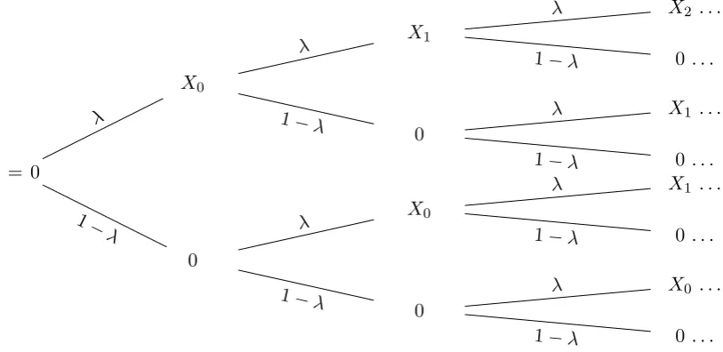
As discussed, if the trader is slow, he does not have access to the HFT technology and cannot observe all trading venues instantaneously. Thus, he may sometimes send orders to a trading venue which is not liquid. He can only send orders to one trading venue in any instant. If he sends an order to some venue at some instant t, it will be executed with probability λ. If it is not executed, I assume that the trader continues to search for a liquid venue for that order until it is executed. To describe the process, I let the dependence on time be explicit so thatXt

denotes the value ofX at timet. The process works as follows (a graphical depiction of which is given in Fig. 1 below):

• At t= 0: the trader submits an order which delivers a profit X0 with probability (w.p.)

λ, otherwise gets 0.

• At t= 1 the trader will do one of the following:

1. If his order is executed att= 0, he submits another order at t= 1 which will yield, if filled,X1. It gets filled with probabilityλ.

2. If, however, his t = 0 order is not filled, at t= 1 he is searching for a liquid venue for his t= 0 order and gets it filled w.p. λ. If filled, it yields the profit X0.

Thus,

E0[X₁S] =λ2E0[X1] + (1−λ)λX0

=λX0(λeµ+ (1−λ))

(2)

sinceX1 and X0 are governed by (1).

Therefore, for some arbitrary instant t≥0, the search process described implies that

E0[X_tS] =λ(1−λ)tX0

t

X

i=0

t i

λeµ

1−λ

i

=λX0((1−λ) +λeµ)t

(3)

by the Binomial theorem.

If, however, the trader is fast, he gets his order filled with certainty whenever he sends it to the market because he can observe which venues are liquid. Thus, he does not need to search for liquidity and at every instantt that he trades, he gets a profit ofXt. Thus, XtF ≡Xt and

E0[X_tF] =X0eµt, (4)

which is, in fact, Eq. (3) for λ= 1.

Moreover, since λ < 1, E0[X_tF]> E0[X_tS] for all t. This says if the trader is fast, he has higher trading profits in expectation than if he were slow because his execution delay costs are zero. This is intuitive and necessary because if this condition did not hold, investment in the HFT technology would never be optimal.

2.2.2 Prevalence of HFT in Market

Much of the literature in this area documents that HFTs generate adverse selection costs for slow traders because their accelerated access to value-relevant information for the asset implies they profit more at the expense of slow traders (see, for example, empirical studies by Baron et al. [2] and Brogaard et al. [5]). Moreover, as documented in Biais et al. [4], anecdotal evidence suggests that the profitability of HFTs has declined in recent years which may be due to the fact that the prevalence of high frequency trading in the market place has increased. I capture these stylized facts by assuming that X0 := (1 +α)−1x, for some x > 0, and where I define

α <1 as the fraction of HFT activity in the market at each instant. Therefore, since the profit

processes both follow a geometric Brownian motion, the current (discounted) expected profit from trading foreach type of trader, for any future time, decreases in the level of HFT activity.

I should point out here that since a higher level ofαis simply equivalent to a lower initial level of the profit process, this parameter is of particular interest in Section 4, where I examine the equilibrium level of fast trading in the market, as well as the trading industry value maximising level.

3

The Optimal Stopping Problem

a fast trader. From time τ onwards, the present value of the investment opportunity is the expected discounted profit flow of a fast trader2; i.e.;

V(x) =E0

Z τ

0

e−rtX_tSdt+

Z ∞

τ

e−rtX_tFdt−e−rτI

(5)

whereEt0 denotes the expectation operator applied at timet0.

Using the strong Markov property of diffusions, we can re-write Eq. (5) as

V(x) =E0

Z ∞

0

e−rtX_tSdt−

Z ∞

τ

e−rtX_tSdt+

Z ∞

τ

e−rtX_tFdt−e−rτI

=E0

Z ∞

0

e−rtX_tSdt

+E0

e−rτEτ

Z ∞

0

e−rt X_tF −X_tS

dt−I

.

(6)

The problem is to find a value function V∗(x) and a stopping time τ∗ > 0 such that the following optimal stopping problem is solved:

V∗(x) = sup

τ∈T

E0[e−rτF(X_τS, X_τF)], (7)

forT the set of stopping times, and

F(X_τS, X_τF) =Eτ

Z ∞

0

e−rt X_tF −X_tSdt

−I (8)

is the trader’s payoff from adopting the technology. Hereafter I denote F(X_tS, X_tF) by F(Xt)

since both XS and XF are functions ofX.

By Fubini’s theorem, and using Eqs. (3) and (4), Eq. (8) can be re-written as

F(Xτ) =Xτ

1

δ −λ

Z ∞

0

e−rt(1−λ) +λer−δtdt

−I

=Ω(r, δ, λ)Xτ−I

(9)

whereδ :=r−µ >0 is the convenience yield (or shortfall)3_{, and the scaling term}

Ω(r, δ, λ) = 1

δ −

λ

(r−ln ((1−λ) +λer−δ₎₎ >0 (10)

represents the relative advantage (in terms of profits) from being fast. Note that I have replaced

µ by r−δ for the purpose of analysing the solution and comparing it with that obtained in a standard real options model with the payoff flow being obtained in perpetuity. Hereafter,δwill be referred to as the “shortfall”.

I present the derivation of Eq. (10) in Appendix A, where I also prove that Ω(r, δ, λ)>0.

2

This is essentially an exchange of one profit flow for another by paying a fixed cost; see for example Dixit and Pindyck [8] Chapter 9, Section 3. However, in that example, there are two investors in a particular project and the leader’s profit flow is exchanged for a different (lesser) profit flow once the follower invests.

3

The relative advantage of being fast is induced by the elimination of delayed execution arising from the need to search for quotes in fragmented markets.

Theorem 1. Let β1>1 be the positive root of the quadratic equation

Q(β) = 1 2σ

2_{β(β−1) + (r−δ)β−r= 0. (11)}

Investment takes place at the first passage time τ∗= inf{t:Xt≥X∗}, for some constant

X∗ = β1

β1−1

(Ω(r, δ, λ))−1I. (12)

Moreover, the optimal stopping problem (7) is solved by

V∗(x) =

 



λ(1+α)−1_x

(r−ln((1−λ)+λer−δ₎₎+

_(1+α)−1_x

X∗

β1

F(X∗) if x <(1 +α)X∗

(1+α)−1_x

δ −I if x≥(1 +α)X

∗_,

(13)

where F(X) is given by Eq. (9).

Proof. See Appendix B.

3.1 Comparative Statics

In this subsection I discuss the economics underlying the optimal investment strategy.

First I discuss the effects of the two HFT related parameters, α and λ, on the optimal investment threshold X∗.

Proposition 1. An increase in the level of fast trading activity, α, and an increase in the probability of finding a liquid venue, λ, makes it optimal for a slow trader to wait longer before investing.

The level of HFT activity in the market does not directly affect the profit threshold X∗

above which it is optimal to become fast. However, an increase in the level ofα reduces a slow trader’s current profit from trading since X0 := (1 +α)−1x. Therefore, the slow trader will

have to wait longer before it is optimal to invest since an increase in α increases the distance between the current profit level and X∗.

The probability of finding a liquid venue impacts the optimal threshold via its effect on the relative advantage of being fast; in particular, through its effect on Ω(r, δ, λ). The relative advantage of being fast is high when the probability of finding a liquid venue is low and thus, it is optimal to invest sooner if the probability of finding a liquid venue decreases. This is because it becomes harder for the slow traders to find quotes quickly and owing to the search process, the more they lag behind the HFTs in terms of trading profits, i.e.;E0[XF]−E0[XS] decreases in the probability of finding a liquid venue.

threshold. The results, are interesting in their own right because they differ somewhat from their effects on the investment threshold in the more standard real options investment model (see for example, Dixit and Pindyck [8], Chapter 6) as I discuss below, but they are also useful in understanding the driving forces underlying the extent of over- and under-investment in the HFT technology in equilibrium, relative to the trading industry welfare maximising level of investment, which I discuss in Section 4.2.

Proposition 2. The optimal investment thresholdX∗ increases in the uncertainty in the profit process σ. Moreover, X∗ increases in the discount rate r and decreases in the shortfall δ when the probability of finding a liquid venue is low, and vice versa when this probability is high.

Proof. See Appendix C.

The effect of uncertainty on X∗ is as expected from other standard models of investment under uncertainty (see for example, Dixit and Pindyck [8] and McDonald and Siegal [17]). It impacts the threshold via the value of waiting. In particular, the more volatile are the profits from trading, the greater is the opportunity cost of investing in the technology since the cost of doing so is high and the investment, once made, is irreversible.

The discount rate and the shortfall impact the optimal threshold X∗ via their effect on the value of waiting (the option effect) and their effect on the present value of the difference in perpetuity factors of fast and slow traders (i.e., its effect on Ω(r, δ, λ))

The equilibrium relationship δ = r−µ must be maintained. Therefore, if r increases, so too does the rate of growth of profit from being fastµand, hence, the expected appreciation in the value of the option to invest in the HFT technology increases making it costlier to invest immediately rather than to wait. However, ifδ increases while keeping the discount rate fixed,

µ will decrease implying that it is costlier to wait rather than to invest immediately because the expected appreciation in the value of the option to invest decreases.4

However, an increase in r also increases the present value of the relative advantage of being fast whenδ is fixed (cf. Eq. (C.4) in Appendix C). This is because the expected present value of a fast trader’s profit flow does not change when the shortfall is constant, but an increase inr

reduces the expected present value of a slow trader’s profit flow. Hence, the relative advantage of being fast increases implying earlier investment is optimal. On the other hand, an increase inδ, while keepingr fixed, reduces the present value of the relative advantage of being fast (cf. Eq. (C.6) in Appendix C) because it reduces the expected present value of a fast trader’s profit flow more than it increases the expected present value of a slow trader’s profit flow. This is because an increase inδ is synonymous with a decrease in the rate of profit growth from being fast. Thus, an increase in δ implies waiting longer is optimal.

4_{We can verify both of these results technically since}

∂ ∂r

β1 β1−1

=− 1

(β1−1)2 ∂β1

∂r >0

and

∂ ∂δ

β1 β1−1

=− 1

(β1−1)2 ∂β1

∂δ <0

So long as the probability of a slow trader finding a liquid venue λ is very low, then the relative advantage of being fast will always remain high so that any change in either r orδ will not significantly impact Ω(r, δ, λ). Therefore, the effect of any shift in either of the parameters on the value of waiting dominates its effect on the relative advantage of being fast. This implies that an increase inrmakes waiting longer optimal, but an increase inδmakes earlier investment optimal when λis low owing to the option effect.

On the other hand, when the probability of a slow trader finding a liquid venue is high, then value of waiting will always be high and this will not be impacted significantly by any shift in

r or δ. Hence, the effect of a change in r or δ on the relative value of being fast dominates their effects on the value of waiting implying that an increase inr will make earlier investment optimal and an increase in δ will make waiting longer optimal in this case, both owing to the present value effect.

The results with respect to r and δ are particularly interesting from the real options per-spective because they differ from more standard result on the (positive) effects of the discount rate (when δ is fixed) and the shortfall (when r is fixed) on the optimal investment threshold when the post-investment profit flow is received in perpetuity rather than as a lump sum payout (see, for example, Dixit and Pindyck [8], Chapter 6).

In their model, the effect ofr on the threshold is always via its effect on the value of waiting when the shortfallδ is kept constant. This is because the pre- and post- investment profit flows are linear functions of the underlying geometric Brownian motion, implying that the present value of the investment is unaffected by changes in r when δ is fixed. Hence, all the impact of

r on the threshold comes from its effect on the value of waiting. However, in my model, the post-investment profit flow is a linear function of the geometric Brownian motion describing the profit flow, but the pre-investment profit flow is not. This is because the slow trader must search for quotes in order to find a liquid venue. Hence, the present value of investing is not unaffected by a change inr in this model and, therefore, the non-linearity of the pre-investment profit flows, as a result of the search procedure, implies that the threshold may increase or decrease in r owing to the option or present value effects, respectively.

In the case ofδ, there are two opposing effects in the Dixit and Pindyck [8] model also, but the present value effect always dominates the option effect so that an increase inδalways implies waiting longer is optimal. This corresponds with my result for a highλ, but an additional effect whereby early investment is optimal will be generated in my model when the probability of finding a liquid venue is low. This is because I include in the model the search procedure for slow traders when finding liquid venues is not certain, and this produces the additional effect.

4

Levels of Fast Trading

To determine the equilibrium level of fast trading, I adopt the same definition of the equi-librium as Biais et al. [4]. They define it as the level ofα such that theex ante expected payoff from fast trading is exactly equal to theex ante expected payoff from slow trading. Ex ante, in the context of the model, means before a trader earns any profit from trading; i.e., when he is neither fast nor slow. Therefore, prior to earning any profit, a trader knows that once he earns a profitXt at some time t≥0, ifXt≥X∗, it will be optimal for him to be fast, otherwise it is

optimal for him to be slow (cf. Theorem 1). (Note that Xt here corresponds directly with the

initial profit level X0 in the optimal stopping analysis.) However, there are a range of values

Xtcan take over which it is optimal to be slow, and another range over which it is optimal for

him to be fast. To capture this variation in possible values, I denote his time t profit level by

X_ti= (1 +α)−1xi_t, for i= 1,2, . . ., and such that the xi_t’s are i.i.d. and continuously distributed on [0,x¯] with ¯x >(1 +α)X∗, and have cumulative distribution functionG(·) and densityg(·).

The trader’s ex ante expected payoff from being fast and from being slow over all possible time t profit levels are denoted by Vf(α) and Vs(α), respectively. Thus, conditional on the optimal strategy defined in Theorem 1:

Vf(α) =E0

h

e−rt V∗(xi_t) +I

x

i

t≥(1 +α)X ∗i

=e−rt

Z x

(1+α)X∗

h

V∗(xi_t) +I

x

i

t≥(1 +α)X ∗i

gf(xi_t)dxi_t

(14)

and

Vs(α) =E0

h

e−rtV∗(xi_t)

x

i

t<(1 +α)X ∗i

=e−rt

Z (1+α)X∗

0

h

V∗(xi_t)

x

i _{<(1 +α)X}∗i

gs(xi_t)dxi_t,

(15)

whereV∗(xi_t) is given in Eq. (13), andgf(·) andgs(·) denote the particular value of the density function which pertains to fast and slow trading, respectively. E0 denotes the expectation

operator applied at time 0.

I denote the ex ante expected relative advantage of fast trading in the market by ∆(α), where

∆(α) :=Vf(α)−Vs(α).

4.1 Equilibrium Fast Trading

As mentioned above, in the manner of Biais et al. [4], I define the equilibrium level of fast trading, denoted byα∗, as the level ofαsuch that the ex ante expected relative advantage from fast trading is equal to the cost of investing. Therefore, if the level of fast trading is α∗ at time

t, then

Vf(α∗)−e−rtI =Vs(α∗)

Thus, if the trader earns a profit at time t and if the level of HFT is α∗, if xi_t = (1 +α∗)X∗, he will be indifferent about being fast or slow, ifxi_t>(1 +α∗)X∗, it will be optimal to become fast, otherwise it will be optimal for him to be slow. However, the level of HFT will be an equilibrium level according to the equilibrium definition.

Now from Eq. (16), it is clear that in determining α∗, the discount factors will cancel out because the discount factor is the same irrespective of whether the trader is fast trading or slow trading. Therefore, the equilibrium results are independent oft, so in the analysis that follows I drop the notational dependence ont.

Proposition 3. There is always a unique equilibrium level of fast trading. If (i) ∆(1)< I <

∆(0), then 0< α∗ <1; (ii) ∆(0)≤I, α∗= 0; or (iii) ∆(1)≥I, α∗ = 1.

Proof. See Appendix D.

The fact that there is always uniqueness of equilibrium is novel. The uniqueness arises from the fact that the ex ante expected relative value of being fast always decreases in α when

∆(1) < I < ∆(0) which, in turn, arises from the optimal stopping rule. If α increases, then

the initial profit level of a trader, irrespective of whether he is fast or slow, decreases. However, this increase in α increases the range of initial profit levels over which it is optimal to be slow ([0,(1 +α)X∗)), the overall effect being an increase in Vs(α). On the other hand, an increase in α reduces the range of profit levels over which it is optimal to be fast ([(1 +α)X∗,x¯]) and thereby reduces Vf(α). Overall, therefore, ∆(α) decreases everywhere in α. Moreover, in this sense, we can say that HFT induces a positive externality on slow trading in the market and a negative externality on fast trading.

If ∆(0)≤I, then the ex ante expected relative value of being fast is low if all trading activity in the market is slow. Therefore, all traders are better off being slow if all other traders are also slow so that α∗ = 0.

If ∆(1)≥I, then the ex ante expected relative value of being fast is high when all trading activity in the market is fast. Hence, everyone is better off being fast so that α∗ = 1.

Multiple equilibria can arise in other financial market models because of virtuous or vicious circles. For example, in Glosten and Milgrom [12] and Dow [9], if traders anticipate the market will be liquid, they will submit many orders, and hence, the market is liquid, and vice versa. In a similar vein, in Biais et al. [4], one equilibrium can arise in which no trader invests because each expects others not to invest, and one in which all traders should become fast because all expect everyone else to be fast. This situation of multiple equilibria arising from self-fulfilling cycles could only arise in the current model if ∆(α) were to increase in the level of HFT for some values of α. In that case, it would be possible to have three equilibria at any instant because if ∆(α) increases in α, then it is possible that ∆(0) < I < ∆(1) could arise. In that case,

α∗ = 0 would be an equilibrium (see reasoning above), α∗ = 1 would be another, and a third

Proposition 4. The equilibrium level of fast trading never increases in the probability of finding a liquid venue.

Proof. See Appendix E.

This result is intuitive and the reasoning is as follows. A decrease in the probability of finding a liquid venue implies earlier investment is optimal (cf. Proposition 1). Thus, the ex ante expected payoff from investing relative to not investing decreases in the probability of finding a liquid venue and, as discussed, this ∆(α) decreases inα. Hence, for equilibrium to be maintained, α∗ must increase in response to a decrease in λ, and vice versa. However, as long as ∆(0)< I, irrespective of a change inλ,α∗ = 0, and similarly,α∗= 1 for all ∆(1)> I. In the interior region where ∆(1)< I <∆(0), we experience the actual negative relationship between

λon α∗.

4.2 Socially Optimal versus Equilibrium Fast Trading

The socially optimal level of fast trading is the level of α that maximises a trader’s ex ante utilitarian welfare. Say the level of HFT in the market at time t isα. Then ex ante, a trader expects the payoff from fast trading to be Vf(α)−e−rtI, which the fractionα of all trader’s in the market earn in expectation, and Vs(α) is the ex ante expected payoff earned by the remaining fraction 1−α of traders. Hence, the ex ante utilitarian welfare is given by

W(α) =αVf(α)−e−rtI+ (1−α)Vs(α)

=α ∆(α)−e−rtI

+Vs(α).

(17)

Denoting the socially optimal level of fast trading in the market by αSO, then αSO solves

W0(αSO) = ∆(αSO)−I−

−αSO∂V f_(α)

∂α |α=αSO−(1−α

SO₎∂Vs(α)

∂α |α=αSO

= 0, (18)

whereW0(αSO) =∂W_∂α(α)|_α=αSO, and the difference between the equilibrium level of fast trading

and the socially optimal level is driven by the term in brackets. This term can be positive or negative since Vf(α) decreases and Vs(α) increases in α (cf. Appendix D). It will be positive (resp. negative) if the impact ofαonVf(α) (resp. Vs(α)) dominates its impact onVs(α) (resp.

Vf(α)) and the overall effect of HFT is therefore a cost (resp. benefit) to society. Hereafter, I refer to it as the externality effect and denote it by E.

Note that the discount factor drops out when determining αSO in Eq. (18) , so in the following analysis of the socially optimal level, I omit the notational dependence on t.

The socially optimal level of HFT is not necessarily zero. If the socially optimal level were to be zero, then the following condition would have to hold: W0(0) = ∆(0)−I+∂V_∂αs(α)

α=0 = 0.

that it is the relative gain from fast trading which gives HFT its social value in the model. This relative gain is owing to the reduction in delay costs which trading in fragmented markets can inflict on those without access to the technology.

On the other hand, it would be socially optimal for all traders in the market to be fast if

W0(1) = ∆(1)−I+∂V_∂αf(α)

α=1= 0 holds. However, as shown in Appendix D,∂V

f_{(α)/∂α <0}

for allα, the condition will not be satisfied if ∆(1)−I <0; i.e., if the ex ante expected relative value of fast trading in the market is low when everyone if fast. Thus, it is not socially optimal for all traders to be fast when the expected relative value of fast trading in the market is low if everyone in the market is fast.

Proposition 5. When the cost of investing in the HFT technology is low, the equilibrium level of fast trading is never lower than the socially optimal level. However, for sufficiently high levels ofI, the equilibrium level will be lower than the socially optimal level. Moreover, there is always a cost level such that the equilibrium level and the socially optimal level coincide.

The reasoning is as follows. If the effect of a change in α on Vf(α) dominates its effect on Vs(α), then the externality effect E is positive and there is an over-investment in the fast trading technology in equilibrium relative to what is socially optimal. This happens when I is low because the low cost implies a low value of waiting. Thus, the ex ante expected relative value of being fast is high. From Eq. (18) and the equilibrium condition that ∆(α∗)−I = 0, it must be the case therefore that ∆(αSO)>∆(α∗). Since ∆(α) decreases inα (see Appendix D), thenαSO_{< α}∗_.

The over-investment in speed in equilibrium relative to the socially optimal level result has been found in other papers, but for different reasons to the one in this paper. See, for example, Budish et al. [6] who develop a model in which traders invest in speed so that they can quickly react to the arrival of public information but, in contrast to this model, gains from trade are not modelled. This absence in trading gains leads to a result that slow trading is always socially optimal. In Biais et al. [4], each investor also chooses his speed at which it operates in a given market, but in that paper, over-investment in speed always arises and that is because fast traders benefit from the adverse selection cost they inflict on slow traders, but they do not internalise this cost in equilibrium. This increases the level of HFT in equilibrium, but the socially optimal level does not increase in the benefits from adverse selection. Hence, over-investment arises. Moreover, Glode et al. [11] view investment in HFT as an arms race, and there is an equilibrium in which every investor chooses to invest in the technology in the fear others will also do so, which leads to over-investment.

On the other hand, if the effect of a change in α on Vs(α) dominates its effect on Vf(α),

E is negative and there is an under-investment in equilibrium relative to the socially optimal level. This occurs when I is high since waiting to invest is optimal. By a similar reasoning to the over-investment case,αSO> α∗; i.e., there is an under-investment in equilibrium.

trade only in slow markets which, in turn, reduces the expected profits of HFTs. In their extended model, only two types of equilibria can arise: all traders trade in slow markets or all are fast. By contrast, under-investment can occur in my model without considering the possibility of slow only markets. This is because I view investment in the HFT technology as an optimal stopping problem and, owing to the inclusion of the value of waiting, under-investment can occur in equilibrium (and not necessarily either an all fast (α∗ = 1) or all slow (α∗ = 0) equilibrium) when the cost of investing is very high. In my case, when under-investment arises, it does so because, for a given level of fast trading α∗, it is not optimal for enough traders to avail of the reduction in delay cost which investment would provide because the benefit of this reduction is not sufficiently high to warrant paying such a high investment cost owing to the value of the option to wait.

Therefore, owing to the optimal timing policy, it is the case that for some levels of investment

costαSO< α∗, and for other levels α∗ > αSO, implying there is a uniqueI such that α∗ =αSO

and this is the level ofI such that the externality effect is zero; in other words, the level of I

such that

∂Vf(α)/∂α

∂Vs_(α)/∂α|α=αSO = 1−

1

αSO.

Another interesting question is how the regions of over and under-investment in equilibrium are related to changes in the standard real option parameters r,σ, and δ (via a change in µ). In essence, we want to understand how shifts in these parameter values impact the extent of over- and under-investment. The following proposition summarises the impact they have.

Proposition 6. The extent of over-investment decreases and the extent of under-investment increases inr andσ. The extent of over-investment and the extent of under-investment decrease in δ.

Proof. See Appendix F.

This result is driven by the impact of the parameters on the externality effect E (i.e., the bracketed term in Eq. (18)). As discussed, when E >0, the externality cost of HFT incurred by fast traders dominates the externality benefit of HFT acquired by slow traders and there is over-investment in equilibrium. On the other hand, when E < 0, the externality benefit dominates the externality cost, and there is under-investment. Therefore, over-investment will be alleviated when any parameter shift leads to a reduction in E, and under-investment will be alleviated when there is an increase in E. However, if the externality effect increases or decreases, so too must ∆(α) so that the socially optimal condition (18) is maintained. Thus, we can interpret the effects of the parameters on the extent of over- and under-investment by examining the impact of a parameter shift on ∆(α). In essence, a parameter shift that leads to an increase in ∆(α) exacerbates the extent of over-investment and alleviates the extent of under-investment in equilibrium, and vice versa, which is what intuition would suggest.

investment is high and hence, we can infer that the over-investment scenario arises in this case. Thus, when we have over-investment in equilibrium relative to the socially optimal level, X∗

increases inr and σ. However, ∆(α) decreases inX∗ (which is proven in Appendix F) because such an increase reduces (increases) the range of profit levels over which it is optimal to be fast (resp. slow) so that ∆(α) will be lower for some fixedα. Therefore, we can conclude that increases inσ and/orr in the over-investment scenario alleviates the extent of over-investment.

In the case of under-investment, the probability of finding a liquid venue will be high and, therefore, so too will be the optimal investment threshold X∗. The higher the level of the threshold, the more immaterial it is in the sense that as λ → 1, X∗ → ∞, so that for very high probability levels, the investors will not contemplate investing and, hence, the impact of

X∗ on the extent of under-investment is irrelevant. Therefore, the effect of r and σ on the extent of under-investment is via their direct impacts on Vf(α) and Vs(α). In fact, in the under-investment case, the value of being fast is very small relative to the value from being slow (since λis high) so that the effects of the parameters are really via their effects onVs(α) and, in particular, via their effects on the value of waiting (cf. Appendix F). An increase in r

orσ implies the value of waiting increases so that the ex ante expected profit from being slow increases. Therefore, ∆(α) decreases (since their impact on Vf _{is negligible) and the extent of}

under-investment will be exacerbated.

Regarding the shortfall δ, an increase in δ, owing to a decline in the rate of profit growth from being fast, leads to a decrease in the ex ante expected profit from being fast and an increase in the ex ante expected profit from being slow. When we have over-investment,Vf(α) is high relative to Vs(α), so the effect of δ on Vf(α) dominates its effect on Vs(α), and vice versa when we have under-investment. Therefore, an increase inδ leads to a reduction in ∆(α) when we are in the over-investment scenario, and an increase in this value when we are in the under-investment scenario. Hence, an increase inδ alleviates the extent of both over-investment and under-investment in equilibrium.

4.3 Implications for Policy

The analysis so far leads to the inference that one appropriate policy response would be to tax or subsidise HFT activity in a manner akin to imposing a Pigouvian tax or subsidy. This tax (or subsidy), denoted by T∗∗, would align the equilibrium level of HFT with the socially optimal level when it is set equal to the externality effect given by the bracketed term in Eq. (18); i.e., E. Note that when E >0, we have over-investment in equilibrium relative to the socially optimal level, so T∗∗ would take the form of a tax, but when E < 0 it would be a subsidy. The result from Proposition 5 indicates that the tax will be higher when the cost of investment is low because this encourages early investment in the HFT technology, and overall leads to over-investment in equilibrium relative to the socially optimal level. On the other hand, for sufficiently high levels of investment cost, the cost should actually be subsidised to encourage slow traders to invest sooner so that they avail of the reduction in delay cost that HFT provides in fragmented markets.

when the cost is low will deter slow traders from adopting the technology as it essentially increases the cost of investing making waiting relatively more valuable, but it will not reduce the level of HFT that is already prevalent because there is no incentive with such a policy for HFTs to stop “trading fast”. Such a caveat does not arise in the under-investment case because reducing the cost of investment by a subsidy will make investing relatively more attractive to slow traders.

One way of circumventing the issue in the over-investment case would be to subsidise HFTs to stop trading fast. This subsidy,S∗∗ would need to be large enough so that the HFTs are at least indifferent between being fast or slow; i.e., S∗∗ is such that

Vs(α) +S∗∗≥Vf(α)−I.

If|S∗∗|=|T∗∗|, then the level of HFT in equilibrium will also be socially optimal.

5

Concluding Remarks

In recent years, the state of market microstructure has changed considerably. There are many ways in which these changes have come about, but one of the biggest changes is that markets have become highly fragmented. When markets are fragmented, traders must search across many markets for venues which will execute their orders at their specified prices. This can result in delayed or partial execution which is costly. In response to the increase in market fragmentation, there has been a demand for speed by traders, and various types of expensive technologies have been developed. Such technologies enable traders to compare all trading venues instantaneously or obtain a glimpse of the true state of the market before everyone else.

In this paper I derive a dynamic model, using techniques from real options analysis, which provides an optimal timing strategy for slow traders to invest in a high frequency trading technology. The model prescribes waiting longer to invest if the level of high frequency trading in the market increases, and it prescribes earlier adoption if the probability of finding a liquid venue decreases. It also prescribes waiting longer if the uncertainty of the profit process increases and, if the probability of finding a liquid venue is low, if the discount rate increases and/or the shortfall decreases. However, if the probability of finding a liquid venue is high, an increase in the discount rate and a decrease in the shortfall make early adoption optimal.

of under-investment. However, both under- and over-investment are alleviated by increases in the shortfall. All of these results are driven by the optimal timing policy.

Finally, I discuss why a Pigouvian subsidy given to slow traders to encourage investment when the cost of investment is high is a reasonable policy response to aligning the equilibrium level of HFT with the socially optimal level in the case of under-investment, but that a Pigouvian tax imposed on fast traders when the cost is low, may not be the most effective means of obtaining alignment in the case of over-investment. However, subsidising HFTs to refrain from trading fast (i.e., trading using their fast technology) may be effective in that instance.

It is clear that further research on this issue is warranted and one possibility could be to extend the model by assuming regulators impose a stochastic per period tax on HFTs which is positively correlated with the extent to which the equilibrium level and the socially optimal level are misaligned. If the fast trader had then the option to “exit the market”, or in other words, revert to being slow if paying this tax became too costly relative to the benefit from having no delay costs, then this may be a more effective way of aligning market equilibrium with social optimality (than paying the HFTs to “exit” when there is over-investment) because this could then simultaneously change thecurrent level of HFT as well as changing the optimal adoption threshold for slow traders. This would require a high level of surveillance to ensure that those fast traders who no longer pay the “fast tax” also no longer use co-location services, smart routers etc. The approach would also work in the under-investment case because if the subsidy is stochastic and positively correlated with the extent of under-investment, then if the under-investment problem is large, the subsidy would be large enough to encourage a high level of investment, but if the problem is small, it would be small enough to only encourage a small increase. Also, a stochastic subsidy would be unlikely to alter the level of HFT already prevalent because it would not discourage HFTs to refrain from trading fast. Certainly, investigating this type of policy response, along with the potential means of enforcement, is an interesting topic for future research.

Appendix

A

Derivation of

Ω(

r, µ, λ

)

and proof that

Ω(

r, µ, λ

)

>

0

A.1 Derivation

From Eq. (9),

Ω(r, µ, λ) :=

1

δ −λ

Z ∞

0

e−rt((1−λ) +λeµ)tdt

To prove my result in Eq. (10), it is sufficient to simply present my derivation ofR₀∞e−rt((1−λ) +λeµ)tdt

Z ∞

0

e−rt((1−λ) +λeµ)tdt=

Z +∞

0

e−t(r−ln((1−λ)+λeµ))dt

=

− 1

r−ln ((1−λ) +λeµ₎e

−t(r−ln((1−λ)+λeµ))

+∞

0

.

Now

lim

t→+∞e

−t(r−ln((1−λ)+λeµ₎₎

= 0

if and only if r−ln ((1−λ) +λeµ_{)>0. Hence, we must prove that r−ln ((1−λ) +λe}µ_)>0.

If λ = 1, then the latter expression becomesr−µ (= δ) which is positive by assumption. Therefore, if the expression decreases inλ, then it is positive everywhere. Indeed,

∂

∂λ(r−ln ((1−λ) +λe

µ_{)) =} 1−eµ

(1−λ) +λeµ <0

implying r−ln ((1−λ) +λeµ)>0.

Therefore,

Z ∞

0

e−rt((1−λ) +λeµ)tdt= 1

r−ln ((1−λ) +λeµ₎.

A.2 Proof that Ω(r, µ, λ)>0

Ω(r, µ, λ) = 1

δ −

λ

(r−ln ((1−λ) +λeµ₎₎ >0

Ifλ= 1, then Ω(·) = 0. Hence, if Ω(·) decreases inλ, then Ω(·) must be positive.

∂Ω(·)

∂λ <0⇐⇒r−ln ((1−λ) +λe

µ_{) +} λ(eµ−1)

(1−λ) +λeµ >0.

This is true since µ > 0 by assumption and since r−ln ((1−λ) +λeµ) > 0, which is proven above.

B

Proof of Theorem 1

The derivation of the optimal threshold uses well-developed standard techniques from real op-tions theory (see, for example, Dixit and Pindyck [8]).

Once the trader invests in the technology, he obtains a flow of profits of X_tF ≡ Xt in

perpetuity. Thus, the net present value from investing, denoted byVA_(X

0), is given by

VA(X0) =E0

Z ∞

0

e−rtXtdt

−I = X0

δ −I. (B.1)

Prior to investing, the trader obtains a flow of profits XS, as well as having the option to invest. Letting VB_(X

standard dynamic programming arguments from Dixit and Pindyck [8], VB(X0) solves the

following Bellman equation:

1 2σ

2_X2 0(VB)

00

(X0) + (r−δ)X0(VB)0(X0)−rVB(X0) +X0S= 0, (B.2)

where (VB₎00_(X

0) :=∂2VB(·)/∂X02 and (VB)0(X0) :=∂VB(·)/∂X0.

The solution to this equation takes the following general form

VB(X0) =A1X0β1 +A2X0β2 +

XS

0

δ ,

whereA1 andA2 are constants to be determined, andβ1 andβ2 are the two (real) roots of the

quadratic equation:

1 2σ

2_{β(β−1) + (r−δ)β−r= 0.}

Intuitively, the present value of trading for the slow trader ought to be comprised of the expected present value of his profit flow as if he were never to invest in the HFT technology, but adjusted for the fact that he has the option to invest in the technology should the expected payoff from investing become sufficiently large to warrant the cost of doing so (Dixit and Pindyck [8]). Hence, the general form ofVB(X0) should comply with this intuition. To this end the first two

terms are the value of his option to invest, and the termX₀S/δ represents the expected present value of his profit flow as if he were never to invest. Hence, it must be the case that

X₀S

δ ≡E

0Z ∞ 0

e−rtX_tSdt

=λX0

Z ∞

0

e−rt(1−λ) +λer−δtdt

= λX0

r−ln ((1−λ) +λer−δ₎

(B.3)

(cf. Eq. (3) and Appendix A.1 for technical details.)

If the slow trader’s current profit X₀S is zero, it will stay at zero forever because XS must follow a geometric Brownian motion, which has an absorbing barrier at zero, owing to its dependence on X (see Eq. (B.3)). Thus X₀S = 0 iff X0 = 0. However, since X0 ≡ X0F, this

implies that investing and becoming fast will never yield any profit either and, hence, that the value of the option to invest has no value. Therefore, the following condition must be satisfied at the boundary:

VB(0) = 0.

But since β2<0, this condition is satisfied iff A2= 0.

Therefore, a solution to Eq. (B.2) which satisfies to the boundary condition is given by

VB(X0) =A1X0β1+

λX0

r−ln ((1−λ) +λer−δ₎. (B.4)

before and and after investing should meet tangentially. In other words, the following conditions must be satisfied

VB(X∗) =VA(X∗)

and

(VB)0(X∗) = (VA)0(X∗),

where (Vi)0(X∗) = ∂Vi(X0)

∂X0

X0=X∗

(fori={A, B}).

Together these these conditions give

X∗= β1

β1−1

(Ω(r, δ, λ))−1I, (B.5)

and

A1 = (Ω(r, δ, λ)X∗−I) (X∗)−β1 ≡(X∗)−β1F(X∗) (B.6)

where

Ω(r, δ, λ) := 1

δ −

λ

r−ln ((1−λ) +λer−δ₎

andF(X∗) is given by Eq. (9). Finally, sinceX0:= (1 +α)−1x, the result for the value function

which solves the optimal stopping problem can be verified.5

C

Proof of Proposition 2

X∗ = β1

β1−1

(Ω(r, δ, λ))−1I

where

Ω(r, δ, λ) = 1

δ −

λ

r−ln ((1−λ) +λer−δ₎.

(Hereafter I just write Ω in the interest of preserving space.)

Let

Q(β1) :=

1 2σ

2_β

1(β1−1) + (r−δ)β1−r = 0.

Then for ζ ∈ {r, δ, σ}:

∂X∗

∂ζ =−

β1

β1−1

1 Ω2

∂Ω

∂ζI−

1 (β1−1)2

∂β1

∂ζ I

Ω. (C.1)

The first term on the right hand side measures the sensitivity of the threshold with respect to the returns on the investment and is referred to as the present value effect. The second term measures the sensitivity of the threshold with respect to β1 and, thus, measures the option

effect. This decomposition is standard in real options models.

5_{Indeed, using the result in Dixit and Pindyck [8] pp. 315-316, we know thatE}0_[e−rτ_{] =} X0

X∗

β1

, whereτ

is the time of investment. Therefore, (X∗)−β1 _{= (X0)}−β1_E0_[e−rτ_{] = ((1 +α)}−1_x)−β1_E0_[e−rτ_{]. Thus, we can}

writeA1 asA1=E0_[e−rτ_{] (1 +α)}−1_x−β1_F(X∗

Now

∂β1

∂ζ =−

∂Q(β1)/∂ζ

∂Q(β1)/∂β1

=−∂Q(β1)

∂ζ

1

σ2 _β

1−1₂

+r−δ

(cf. Dixit and Pindyck [8] pp. 144) so that we can re-write Eq. (C.1) as follows:

∂X∗

∂ζ χ

X∗ =−χ

∂Ω

∂ζ +

Ω2

β1

∂Q(β1)

∂ζ , (C.2)

where

χ:= (β1−1)

σ2

β1−

1 2

+r−δ

Ω2.

From Eq. (C.2), since∂Ω/∂σ = 0 and∂Q(β1)/∂σ =σβ1(β1−1)>0,

∂X∗

∂σ >0

owing solely to the option effect.

Also, from Eq. (C.2), we see that

∂X∗

∂r >0⇐⇒

Ω2

β1

(β1−1)> χ

∂Ω

∂r (C.3)

where the right hand side of the second inequality in (C.3) gives the present value effect and the left hand side the option effect. Moreover,

∂Ω

∂r =

λ(1−λ)

(r−ln ((1−λ) +λer−δ₎₎2_(1−λ+λer−δ₎ >0. (C.4)

If Ω is large, then the option effect will dominate and therefore drive the effect ofr on X∗. In this case,X∗ will increase inr.

However, ifλis high, and Ω is therefore small, then we have thatX∗ will be impacted byr

owing to the PV effect because Ω increases inr. In this case, X∗ will decrease in r.

∂X∗

∂δ >0⇐⇒χ

∂Ω

∂δ + Ω

2_{<0 (C.5)}

where

∂Ω

∂δ =−

1

δ2 +

λ2er−δ

(r−ln ((1−λ) +λer−δ₎₎2_(1−λ+λer−δ₎ <0 (C.6)

(since∂Ω/∂δ is continuous inλand ∂Ω/∂δ= 0 for λ= 1 and ∂Ω/∂δ=−1/δ2<0 for λ= 0).

D

Proof of Proposition 3

First I use Leibniz rule for differentiating integrals to show that ∆(α) decreases inα.

∂∆(α)

∂α =

∂Vf(α)

∂α −

∂Vs(α)

∂α

=− 1

δ(1 +α)2

Z x¯

(1+α)X∗

xigf(xi)dxi− (X

∗₎2

δ g

f_{((1 +α)X}∗

)

−h− λ

(1 +α)2

1

(r−ln ((1−λ) +λer−δ₎₎

Z (1+α)X∗

0

xigs(xi)dxi

+ λ(X

∗₎2

(r−ln ((1−λ) +λer−δ₎₎g

s_{((1 +α)X}∗₎

−β1(1 +α)−β1−1(X∗)−β1F(X∗)

Z (1+α)X∗

0

(xi)β1_gs_(xi_)dxi

+X∗F(X∗)gs((1 +α)X∗)i,

(D.1)

where the term in the square brackets is∂Vs(α)/∂α.

It is clear from the equation that∂Vf(α)/∂α <0. Then it must be the case that∂∆(α)/∂α <

0 if ∂Vs(α)/∂α >0.

∂Vs(α)/∂α >0 if

(X∗)2gs((1 +α)X∗)> 1

(1 +α)2

Z (1+α)X∗

0

xigs(xi)dxi (D.2)

and if

X∗gs((1 +α)X∗)> β1(1 +α)−β1−1(X∗)−β1

Z (1+α)X∗

0

(xi)β1_gs_(xi_)dxi_{. (D.3)}

Using the integration by parts technique to evaluate the integrals in the latter two equations, it is sufficient to approximate the integrals using only the “uv” term in the standard formula to show the conditions hold if we assume that ∂g_∂xs(xii) ≥0. This is because the “

R

vdu” term is negative. Indeed, there are many specifications ofgs_{(·) such that the derivative is nonnegative.}

For example, assuming the xi’s follow a uniform distribution, gs(xi) = _(1+α1_)X∗, the derivative

of which is zero. Lettingu=gs(xi) anddv =xidxiordv= (xi)β1_dxi_{, then [uv]}(1+α)X

∗

0 = 12(1 +

α)2(X∗)2gs((1 +α)X∗) for Eq. (D.2), and [uv](1+α)X

∗

0 = β11+1(1 +α)

β1+1_(X∗₎β1+1_gs_{((1 +α)X}∗₎

for (D.3).

Eq. (D.2) becomes

(X∗)2gs((1 +α)X∗)> 1

2(X

∗₎2_gs_{((1 +α)X}∗_{), (D.4)}

which clearly holds, and Eq. (D.3) becomes

X∗gs((1 +α)X∗)> β1

β1+ 1

X∗gs((1 +α)X∗), (D.5)

Therefore, ∂Vs(α)/∂α >0 and ∆(α) decreases inα everywhere.

From this, it is clear then that the equilibrium condition

∆(α∗)−I = 0 (D.6)

is satisfied if ∆(0)−I >0 and ∆(1)−I <0 so that there is a unique zero point. If both are true, then the condition must hold for some 0< α∗ <1.

If ∆(0)≤I, then since ∆(α) decreases everywhere inα, it must also be true that ∆(α)≤I. Hence,α∗= 0. If ∆(1)≥I, thenα∗= 1 by a similar reasoning.

E

Proof of Proposition 4

First I determine how ∆(α) is affected by λ.

∂∆

∂λ =

∂Vf

∂λ −

∂Vs

∂λ . (E.1)

We use Liebniz rule once more and recall that ∂X∗/∂λ >0:

∂∆

∂λ =−(1 +α)

∂X∗

∂λ

X∗

δ g

f_{((1 +α)X}∗

)

−

Z (1+α)X∗

0

h

(1 +α)−1 x

i

(r−ln ((1−λ) +λer−δ₎₎2

r−ln(1−λ) +λer−δ

+ λ e

r−δ₋₁

(1−λ) +λer−δ

−β1 (1 +α)−1xi

β1

(X∗)−β1−1∂X

∗

∂λ F(X

∗₎i_gs_(xi_)dxi

+ (1 +α)∂X

∗

∂λ

h λX∗

(r−ln ((1−λ) +λer−δ₎₎+F(X

∗₎i_gs_{((1 +α)X}∗_).

(E.2)

This expression is definitely negative if

(1 +α)∂X

∗

∂λ

h λX∗

(r−ln ((1−λ) +λer−δ₎₎ +F(X

∗₎i_gs_{((1 +α)X}∗₎

>β1(1 +α)−β1(X∗)−β1−1

∂X∗

∂λ F(X

∗₎

Z (1+α)X∗

0

(xi)β1_gs_{((1 +α)x}i_)dxi_.

(E.3)

As in Appendix D, assuming the derivative ofgs(xi) is nonnegative, it is sufficient to approxi-mate R₀(1+α)X∗(xi)β1_gs_{((1 +α)x}i_)dxi _{by (β}

1+ 1)−1(1 +α)β1+1(X∗)β1+1gs((1 +α)X∗) since the

remaining term is negative. Replacing for this in the latter equation gives

λX∗

(r−ln ((1−λ) +λer−δ₎₎ >−

1

β1+ 1

F(X∗), (E.4)

which clearly holds. Therefore, this implies that ∆(α) decreases inλ.

˜

α <αˆ. Therefore,α∗ decreases inλ.

F

Proof of Proposition 6

From Eq. (18), we see that if ∆(α) increases owing to a shift in any of the parameter values, then so too must the externality effect E (the bracketed term in this equation) so that the socially optimal condition is satisfied. When E= 0, then α∗=αSO. IfE >0, over-investment in equilibrium arises and any parameter shift that forcesEto increase will exacerbate the extent of over-investment. WhenE <0, under-investment arises, and any parameter shift that causes an increase in E will alleviate the extent of under-investment. Therefore, if we examine the effects ofr,δ and σ on ∆(α), we can infer how shifts in these parameters impact the extent of over- and under-investment in equilibrium.

From Eqs. (14) and (15),

∆(α) =

Z ¯x

(1+α)X∗

xi

(1 +α)δg

f_(xi_)dxi

−

Z (1+α)X∗

0

λxi

(1 +α)(r−ln((1−λ) +λer−δ₎₎+

xi

(1 +α)X∗

β1

F(X∗)

!

gs(xi)dxi.

(F.1)

We see from this equation that the parameters impact ∆(α) directly and via their impact on

X∗. Thus, we need to determine how shifts inX∗owing to shifts inr,σ, andδ impact on ∆(α). By Leibniz rule

∂∆(α)

∂X∗ =−(1 +α)

X∗

δ g

f_{((1 +α)X}∗₎

−h

Z (1+α)X∗

0

xi

(1 +α)X∗

β1

F0(X∗)− β1

(1 +α)X∗

xi

(1 +α)X∗

β1

F(X∗)

gs(xi)dxi

+ (1 +α)

λX∗

(r−ln((1−λ) +λer−δ₎₎+F(X ∗₎

gs((1 +α)X∗)i

But F(X∗) = ΩX∗ −I and substituting for R(1+α)X∗

0 (x

i₎β

1gs(xi)dxi (see Appendix D), the

equation reduces to

∂∆(α)

∂X∗ ≈ −

2X

∗

δ −I

(1 +α)gf((1 +α)X∗)− αβ1

β₁2−1Ig

s_{((1 +α)X}∗_)<0

if 2X∗ > δI. This always holds if it holds when X∗ is at a minimum. X∗ will have minimum

value when λ= 0 and, thus, when Ω =δ. Then the latter condition becomes 2β1/(β1−1)>1,

which is satisfied sinceβ1>1. Hence ∆(α) decreases inX∗ everywhere.

(i) Forλlow (over-investment case):

lim

λ↓0∆(α) =

Z ¯x

(1+α)X∗

xi

(1 +α)δg

f_(xi_)dxi₋Z (1+α)X

∗

0

xi

(1 +α)X∗

β1

F(X∗)gs(xi)dxi

and, as before, we approximate the integrals by

Z x¯

(1+α)X∗

xigf(xi)dxi ≈ 1

2

h

¯

x2gf(¯x)−(1 +α)2(X∗)2gf((1 +α)X∗)

i

and

Z (1+α)X∗

0

(xi)β1_gs_(xi_)dxi _≈ 1

β1+ 1

(1 +α)β1+1_(X∗₎β1+1_gs_{((1 +α)X}∗₎

so forλlow

∆(α)≈ 1

2δ(1 +α)

¯

x2gf(¯x)−(1 +α)2(X∗)2gf((1 +α)X∗)− 1 +α

β1+ 1

(X∗)F(X∗)gs((1 +α)X∗)

Thus, we can see from this equation that impact of r and σ on the extent of over-investment will certainly be via their impact on X∗, but the impact of δ could be via its impact on X∗

or directly. However, since X∗ relatively low for λ low, the effect of δ on _2δ(1+1 _α)x¯2gf(¯x) will dominate its effect on the other two terms. Therefore, ifδ increases, ∆(α) will decrease and, as discussed above, so too will E. Therefore the extent of over-investment will be alleviated.

Since we know that X∗ increases inσ and inr when λis low (cf. Proposition 2), the extent of over-investment will decline in σ and r. This is because if r and/or σ increase, so too will

X∗ and, as just shown ∆(α) will decrease. Hence, E will decline also implying a reduction in the extent of over-investment.

(ii) For λhigh (under-investment case):

lim

λ↑1∆(α) =−

Z ∞

0

xi

(1 +α)δg

s_(xi_)dxi_{. (F.2)}

Taking this limit shows that when we have under-investment, or equivalently, the probability of finding a liquid venue is so high that the thresholdX∗ is essentially immaterial, the effect of

r, δ and σ on ∆(α) is owing to their direct effects, rather than via X∗. However, we need to examine the Eq. (F.1) again to understand the direct effects.

We see that, since _r−ln((1−λ_λ)+λer−δ₎ ≈ 1_δ and

xi

(1+α)X∗

β1

≈0 for λvery high, the effects of

r and σ on ∆(α) will be via their effect on F(X∗) =I/(β1−1). So forζ ={r, σ}

∂∆(α)/∂ζ >0⇐⇒∂F(X∗)/∂ζ <0⇐⇒∂β1/∂ζ >0.

However, we showed in Appendix C that β1 decreases in r and σ. Therefore, an increase in r

orσ will lead to a decrease in ∆(α) which will exacerbate the extent of under-investment.