City, University of London Institutional Repository
Citation:
Bredin, D., Cuthbertson, K., Nitzsche, D. and Thomas, D. C. (2014).
Performance and performance persistence of UK closed-end equity funds. International
Review of Financial Analysis, 34, pp. 189-199. doi: 10.1016/j.irfa.2014.05.011
This is the accepted version of the paper.
This version of the publication may differ from the final published
version.
Permanent repository link:
http://openaccess.city.ac.uk/12497/
Link to published version:
http://dx.doi.org/10.1016/j.irfa.2014.05.011
Copyright and reuse: City Research Online aims to make research
outputs of City, University of London available to a wider audience.
Copyright and Moral Rights remain with the author(s) and/or copyright
holders. URLs from City Research Online may be freely distributed and
linked to.
City Research Online:
http://openaccess.city.ac.uk/
[email protected]
Performance and Performance Persistence of UK
Closed-End Equity Funds
Don Bredin
*, Keith Cuthbertson**, Dirk Nitzsche** and Dylan C. Thomas**
This version: 30th January 2014
Abstract:
Using a comprehensive data set of almost 300 UK closed-end equity funds over the period 1990 to 2013, we
use the false discovery rate to assess the alpha-performance of individual funds with both domestic and
other mandates, using self-declared benchmarks and additional risk factors. We find evidence to indicate
that up to 16% of the funds have truly positive alphas while around 3% have truly negative alphas. Positive
post-formation alphas using fund-price returns depend on the factor model used: there is some
positive-alpha performance when post-formation returns are evaluated using a one-factor global model but
substantial positive-alpha performance when using a four-factor global model.
Keywords : closed-end funds, performance, false discovery rate. JEL Classification : C15, G11, C14
* Smurfit Business School, University College, Dublin. ** Cass Business School, City University London.
Corresponding Author:
Professor Keith Cuthbertson, Cass Business School, 106 Bunhill Row, London, EC1Y 8TZ. Tel. : +44-(0)-20-7040-5070,
Performance and Performance Persistence of UK
Closed-End Equity Funds
1. Introduction
In the UK, closed-end funds (CEF) are an asset class which has often been overlooked by investors, who mainly focus on open-end funds. Nevertheless, particularly for retail investors, closed-end funds provide an attractive investment alternative to open-end funds, as fees are often substantially lower. Restrictions on advertising and a less favorable commission structure for financial advisors are reasons why closed-end funds have remained a niche market in the UK asset management industry. Investors in closed-end funds also have to consider changes in the discount, whereby the net asset value (NAV) of the fund and the price of the fund can diverge substantially – hence, the need to distinguish between the NAV return, which measures the performance of the fund manager, and the fund-price return to the investor.
Research on closed-end funds in the UK and US, has focused mainly on causes of the discount (Lee, Shleifer and Thaler 1990; Gemmill and Thomas 2002); relatively few studies focus on the performance of these funds and no studies (to our knowledge) have used closed-end funds to separate skill from luck by applying the false discovery rate (FDR). The impact of ‘luck’ in multiple hypothesis tests arises whenever we ask the question: ‘How many of our statistically significant results are likely to be ‘truly null?’ – that is ‘false discoveries’. In this paper we use the false discovery rate which measures the proportion of lucky funds among a group of funds, whose performance has been found to be statistically significant. We assess the alpha-performance of the UK closed-end funds over the period November 1990 to January 2013 using a monthly data set, free of survivorship bias. If we simply count the number of funds which are found to have a statistically significant performance measure, we run the risk of including funds which are truly null (i.e. Type I errors). For example, suppose the FDR amongst 20 statistically significant positive-alpha funds is 80%, then this implies that only 4 funds (out of the 20) have truly significant alphas - this is clearly useful information for investors. A key issue is whether this correction gives different inferences from the standard approach of simply ‘counting’ the number of significant funds with non-zero abnormal performance.
size, value, and momentum. No other studies, to our knowledge, attempt to measure closed-end fund performance using the funds’ self-declared benchmarks.
We also address the issue of performance persistence. We sort funds into (decile) portfolios based on a number of different metrics which capture the skill of the fund manager (i.e. NAV performance). The portfolios are frequently rebalanced and we then assess the subsequent alpha-performance. This recursive portfolio approach is analysed for a number of different portfolio formation rules and factor models.
From a total of 330 UK closed-end funds, our final sample of around 300 funds over the period November 1990 to January 2013 provides a large comprehensive data set (largely free of survivorship bias). This paper contributes to the literature by assessing individual-fund performance relative to its self-declared benchmark (as well as other risk factors) and adjusts the number of statistically significant alphas for the presence of false discoveries. For individual fund performance we find that around 75% of funds neither statistically beat nor are inferior to their benchmarks – this applies across all three factor models used. Next, there is a much higher proportion of false discoveries among the worst (negative alpha) funds than amongst the best performing funds – so the standard method of simply counting the number of funds with ‘significant’ test statistics can be far more misleading for ‘losers’ than for ‘winners’. Third, the truly significant positive-alpha and negative-alpha funds appear to be concentrated in the extreme tails of the cross-section of fund performance.
For persistence in performance, we find that sorting into decile portfolios on past performance produces some positive post-sort alphas using fund-price returns in a one-factor model but many more statistically significant post-sort alphas when using a four-factor model.
Previous Studies
Studies which investigate possible sources of skillful and unskillful open-end funds are almost exclusively based on US data. Past winner funds attract additional fund flows (Del Guercio and Tkac 2008; Keswani and Stolin 2008; Ivkovic and Weisbenner 2009) and this may lead to diseconomies of scale (Chen, Hong, Huang and Kubik 2004; Yan 2008), dilution effects (Edelen 1999), distorted trading decisions (Alexander, Cici, and Gibson 2007; Coval and Stafford 2007; Pollet and Wilson 2008) or manager changes (Khorana 1996, 2001; Bessler, Blake, Luckoff, and Tonks 2010) – all of which in turn may affect future performance. At the other end of the spectrum, poorly performing funds are subject to ‘external governance’ (fund outflows) and ‘internal governance’ (manager changes) which also influence their future performance (Dangl, Wu and Zechner 2008; Bessler et al. 2010).
Closed-end funds, unlike open-end funds, are never forced to liquidate securities or purchase additional securities due to fund inflows and outflows. Instead, changes in demand for the fund lead to a widening or narrowing of the discount and hence changes in investors’ returns. Persistence in the performance may therefore be stronger than for open-end funds because sentiment in favour of a closed-end fund might lead to an increased demand for the fund by additional (retail) investors which, with a given fund size, may lead to higher future fund returns. In contrast, an increase in demand for a particular open-end fund will be met by an increased inflow and increased purchases across a wide range of stocks, where the future price impact may be relatively small. CEF’s can also invest in illiquid securities (Cherkes, Sagi, and Stanton 2009) and use leverage (Elton, Gruber, Blake, and Shachar 2013) – this may also result in more positive alphas and performance persistence of active strategies, than for open-end funds.
The literature on closed-end fund performance in the US and UK is relatively sparse. Bers and Madura (2000), using US funds with a domestic mandate, find evidence of positive persistence for NAV and fund-price returns, based on the correlation between estimated alphas in successive periods. Positive persistence is also found for US funds with a foreign mandate although the level of persistence is less than that for domestic funds (Madura and Bers 2002). More recently, Elyasiani and Jia (2011) evaluate fund-price and NAV persistence using 86 US equity funds. They find, however, evidence of only very weak persistence when the funds are evaluated against median risk-adjusted industry performance.
data on 9 portfolios with both domestic and international mandates, Bangassa, Su, and Joseph (2012) find mixed evidence on alpha performance which depends upon the investment mandate and the factor model used.
In this paper we add to the literature by assessing the performance of individual UK closed-end funds using their self-declared benchmarks (and other risk factors) after adjusting for false discoveries. We also examine performance persistence using different sorting rules and different factor models for post-formation returns. The paper is organized as follows. In section 2 we briefly discuss the methodology behind the FDR and other methods of controlling for false positives in a multiple testing framework. In section 3 we look at performance models, in section 4 we present our empirical results; section 5 concludes.
2. The False Discovery Rate
The standard approach to determining whether the alpha of a single fund demonstrates skill or luck is to choose a rejection region and associated significance level and to reject the null of ‘no outperformance’ if the test statistic lies in the rejection region - ‘luck’ is interpreted as the significance level chosen. However, using
= 5% when testing the alphas for each of M-funds, the probability of finding at least one non-zero alpha-fund in sample of M-funds is much higher than 5% (even if all funds have true alphas of zero).1 Put another way, if we find 20 out of 200funds (i.e. 10% of funds) with significant positive estimated alphas when using a 5% significance level then some of these will merely be lucky.
In testing the performance of many funds a balanced approach is needed - one which is not too conservative but allows a reasonable chance of identifying those funds with truly differential performance. An approach known as the false discovery rate (FDR) attempts to strike this balance by classifying funds as ‘significant’ (at a chosen significance level) and then asks the question ‘What proportion of these significant funds are false discoveries?’ – that is, those that
are truly null (Benjamini and Hochberg 1995; Storey 2002; Storey, Taylor, and Siegmund 2004). The FDR measures the proportion of lucky funds among a group of funds which have been found
to have significant (individual) alphas and hence ‘measures’ luck among the pool of ‘significant funds’. Storey (2002) and Barras, Scaillet, and Wermers (2010) provide a detailed account of the FDR methodology, so it is only briefly summarized below. The null hypothesis that fund-i has no skill in security selection (alpha) and the alternative of either positive or negative performance is:
1 This probability is the compound type-I error. For example, if the M tests are independent then Pr(at least 1
false discovery) = 1 – (1- )M = z
H
0:
i
0
H
A:
i
0
or
i
0
A ‘significant fund’ is one for which the p-value for the test statistic (e.g. t-statistic on alpha) is less than or equal to some threshold
/ 2
(0
1
). At a given significance level
the probability that a zero-alpha fund exhibits ‘good luck’ is
/ 2
. If the proportion of truly zero-alpha funds in the population of M-funds is
0 then the expected proportion of false positives (or ‘lucky funds’) is:[1]
E F
(
)
=
0( / 2)
If
E S
(
)
i
s the expected proportion of significant positive-alpha funds, then the expected proportion of truly skilled funds (at a significance level
) is:[2]
E T
(
)
E S
(
)
E F
(
)
E S
(
)
0( / 2)
Varying
allows us to see if the number of truly skillful funds rises appreciably with
or not, which tells us whether skilled funds are concentrated or dispersed in the right tail of the cross-sectional distribution. An estimate of the true proportion of skilled (unskilled) funds
A (
A ) in the population of M-funds is:[3]
AT
*
*
A
T
where
* is a sufficiently high significance level which can be determined using the mean squared error criterion (Barras et al. 2010). The expected FDR amongst the statistically significant positive-alpha funds is:
[4]
(
)
0( / 2)
(
)
(
)
E F
FDR
E S
E S
[5]
E T
(
) / (
E S
) 1
FDR
The observed number of significant funds
S
provides an estimate ofE S
(
)
. To provide an estimate of
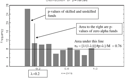
0, the proportion of truly null funds in the population of M-funds, we use the result that truly alternative features have values clustered around zero, whereas truly null p-values are uniformly distributed, U(0,1). To estimate
ˆ ( )
0 we can simply choose a value
for which the histogram of p-values becomes flat and use:[6]
ˆ ( )
0 =( )
#{
}
(1
)
(1
)
i
p
W
M
M
where
W
( ) /
M
is the area of the histogram to the right of the chosen value of
(on the x-axis of the histogram) – see Figure 4. For example suppose
0= 100% and we choose
= 0.2. ThenW
( ) /
M
= 80% of p-values lie to the right of
= 0.2 and our estimate of
0 = 80%/ (1-0.2) = 100% as expected. For truly alternative funds (i.e.
i
0
), the histogram of p-values has a “spike” near zero. But if the histogram of p-values is perfectly flat to the right of
then our estimate of
0 is independent of the choice of
. So, if we were able to count only truly null p-values then [6] would give an unbiased estimate of
0. However, if we erroneously include a few alternative p-values then [6] provides a conservative estimate of
0 and hence of the FDR.The bias in the estimate of
ˆ ( )
0 is decreasing in
(as the chances of including non-zero alpha-funds diminishes) but its variance increases with
(as we include fewer p-values in our estimation). Hence an alternative estimate of
0 is to choose
to minimize the mean-square errorE
{
0( )
0}
2 (Storey 2002, Barras et al. 2010)2 .We use a bootstrap approach to calculate p-values of estimated t-statistics because of the non-normality in regression residuals (Politis and Romano 1994; Kosowski et al. 2006). The
2 Barras et al. (2010) use a Monte Carlo study to show that the estimators outlined above are accurate, are not
estimated factor model of returns is:
r
i t,
ˆ
i
ˆ
i'
X
t
e
ˆ
i t, for i = 1, 2, … M funds, whereT
i =number of observations on fund-i,
r
i,t = excess return on fund-i,X
t = vector of risk factors,e
ˆ
i t,are the residuals and
t
ˆ
i is the (Newey-West) t-statistic for alpha. We draw a random sample (with replacement) of lengthT
i from the residualse
ˆ
i t, and use these bootstrap residualse
~
i,t to generate an excess return seriesr
~
i,t =0
ˆ
i'
X
t
e
i t, under the null hypothesis
i = 0. Usingt i
r
,~
the performance model is estimated and the resulting t-statistic for the alpha-performancemeasure,
t
ib is obtained. This is repeated B = 10,000 times and for a two-sided, equal-tailed test the bootstrap p-value for the alpha of fund-i is:
[7] 1 1
1 1
ˆ
ˆ
2.min[
(
),
(
)]
B B
b b
i i i i i
b b
p
B
I t
t
B
I t
t
where
I
(.)
is a (1,0) indicator variable. The above ‘basic bootstrap’ uses residual-only resampling, under the null of no outperformance (Efron and Tibshirani 1993).3 A similarprocedure is used for other hypothesis tests4.
3. Performance Models
Individual Fund Performance
The performance of individual closed-end funds can be measured using either fund-price returns or NAV returns – the latter measuring the performance of the manager of the fund and the former measuring the return to the investor. The difference between these two measures of performance is the change in the closed-end fund discount.
Our performance models are well known ‘factor models’ and therefore are only described briefly below. When considering the performance of individualfund excess returns we make use of the self-declared benchmark return of the fund (in excess of the risk-free rate),
r
bi t, and consider the following models:3 Alternative bootstrapping procedures such as simultaneously bootstrapping the residuals and the independent variables, or allowing for serial correlation (block bootstrap) or contemporaneous bootstrap across all (existing) funds at time t, produced qualitatively similar results, hence we only report results for the ‘residuals only’ bootstrap.
Excess Benchmark Return Model (EBRM): [8]
r
i t,
r
bi t,
i
i t,One-Factor Benchmark Model (1FBM): [9]
r
i t,
i
1i bi tr
,
i t,Four-Factor Benchmark Model (4FBM):
[10]
r
i t,
i
1i bi tr
,
2iSMB
t
3iHML
t
4iMOM
t
i t,where
r
i t, is the excess return over the risk-free rate, andSMB
t,HML
t andMOM
t are global risk factors which capture size, book-to-market, and momentum, respectively (Fama and French 1993; Carhart 1997). The excess benchmark return model (EBRM) assumes the fund tracks its self-designated benchmark with zero expected tracking error. Recent studies (Sensoy 2009), however, have shown that many funds deviate from their self-declared benchmarks and this is accounted for in the one-factor benchmark model (1FBM) where the benchmark beta is not constrained to be unity, and in the four-factor benchmark model (4FBM) where global risk factors are also included. Equation [10] is widely used to measure open-end fund performance and should also be applicable to closed-end counterparts.Portfolio Performance
In the sample, there are over 100 different self-designated benchmarks. Hence when considering the performance of portfolios of closed-end funds (e.g. equally-weighted portfolios) we cannot use the self-declared benchmark returns
r
bi t, because these may differ for each fund in the portfolio. Instead, we evaluate the return performance of portfolios (in excess of the risk-free rate)r
p t, , using the a global market returnr
m t, (in excess of the risk-free rate) in place of the self-declared benchmark; this gives a one-factor global model, (1FGM). When augmented byt
SMB
andHML
t we obtain our three-factor global model (3FGM). Finally, adding a global momentum variableMOM
t our four-factor global model (4FGM) is:4. Data and Empirical Results
The sample comprises 298 closed-end equity funds traded on the London Stock Exchange. Of these 298 funds, 76 funds have a mandate to invest in UK markets; 59 funds in Far East and Asian markets; 46 funds in global markets and 43 funds in European markets. There are 52 specialist funds, the majority investing in hedge funds or private equity. The remaining 22 funds invest in the US and in emerging markets. There is a degree of subjectivity in this classification. When a fund has a mandate such as, say, ‘Investing in European technology companies’, we classify such a fund as ‘European’. However when a fund has a mandate, say, ‘Investing in technology companies’ but without being restricted to a particular geographic region, such a fund is classified as ‘specialist’. We classify a fund as ‘global’ where it has global mandate but is not restricted to investing in a particular industry or activity.
In cases where the fund declares a particular benchmark, the choice is clear-cut. However in many cases, and particularly early in the sample period, funds did not declare a particular benchmark. In these cases, a benchmark is selected that best matched the investment mandate of the individual fund. Thus, for example, the benchmark selected for Medicx plc - a closed-end fund launched in August 2006 and investing in primary healthcare properties in the UK - is the FTSE All Share Index for Healthcare Equipment and Services. For the 76 funds investing in the UK market, a total of 11 individual benchmarks are used.
Monthly NAV and fund-price returns (including reinvested dividends) for the individual funds are from Datastream. Most of the self-declared benchmarks are available from January 1975, but the global factors used in our multifactor models are only available from November 1990 onwards. Our sample period is therefore from November 1990 to January 2013. The global risk factors are from Kenneth French’s website (converted into pounds sterling) with the one-month LIBOR as the risk-free rate. The analysis includes only those funds with at least 18 monthly observations, giving us NAV returns for 292 funds and fund-price returns for 298 funds; this is close to the entire universe of 330 UK closed-end funds.
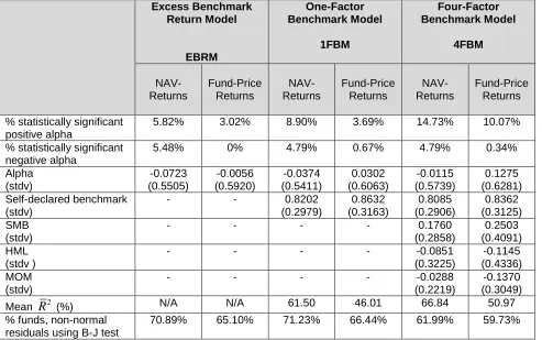
Table 1 reports summary statistics for NAV and fund-price returns over the sample period. Three alternative models are used – the excess return benchmark model (ERBM), the one-factor benchmark model (1FBM) and the four-factor benchmark model (4FBM).
We consider first the results for NAV returns. The number of statistically significant positive alpha funds (at a 5% significance level)increases as we move from the most restricted model to the least restricted model. Thus, as we move from the ERBM to the 1FBM and to the 4FBM, the percentage of statistically significant positivealphas increases from 5.8% to 8.9% to 14.7%, respectively. On the other hand, the percentage of statistically significant negativealphas stays reasonably constant (around 5%) across all three models. The average NAV-return’s alpha across all funds is negative for all three factor models – similar to results reported for open-end funds in the US and UK (see, for example, Kosowski et al. 2006; Cuthbertson et al. 2008; Fama and French 2010). The coefficient on the self-designated benchmark is constant at around 0.81 in the 1FBM and 4FBM models with the latter model indicating a positive loading on
SMB
t and a negative loading on bothHML
t andMOM
t. The averageR
2increases from 61.5% for the 1FBM to 66.8% for the 4FBM - this suggests using the 4FBM when assessing the performance of individual funds. The averageR
2 for closed-end funds is higher than that found when similar factor models are estimated for hedge funds. For example, Capocci and Hubner (2004) report averageR
2 of 44% for a one-factor model and 60% for a four-factor model applied to hedge fund returns.Results for fund-price returns are, for the most part, broadly similar to those for NAV returns although the number of statistically significant positive alphas is smaller while there are no negative alphas. The signs on the three factors are the same as those for the NAV returns but the factor loadings are larger. The average
R
2using fund-price returns is lower than when using NAV returns – implying that the four factors fail to pick up all the variation in the discount. The main difference between the NAV and the fund-price regressions is that the former give negative average alphas whereas the latter give a positive average alpha for the 1FBM (0.36% p.a.) and 4FBM (1.53% p.a.). All three models for individual CEF returns have about 60-70% of funds with (statistically significant) non-normal residuals (Bera-Jarque test, at 5% significance level) – thus motivating the use of bootstrap procedures in testing fund performance.To obtain further insight into the importance of the risk factors in explaining the performance of the average fund, we form an equally-weighted portfolio of all the funds and examine the recursive parameter estimates for the NAV and fund-price returns.
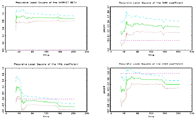
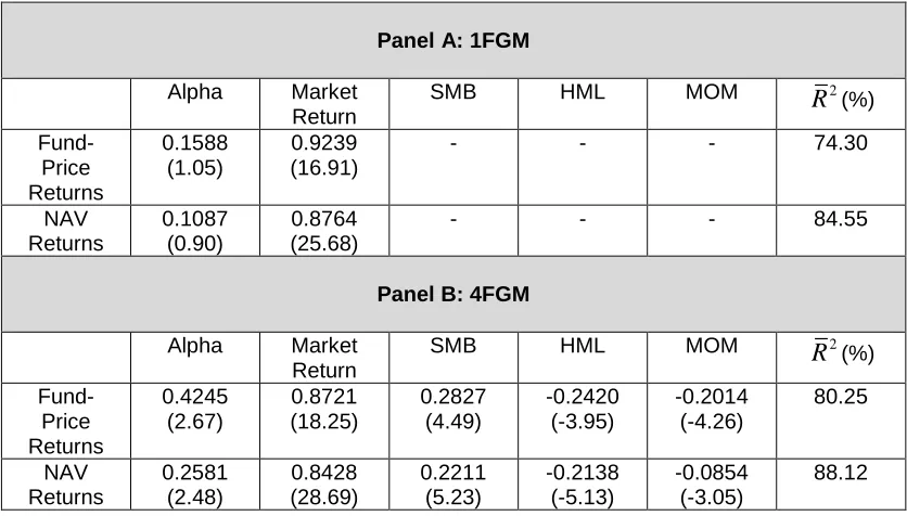
For the one-factor global model (1FGM), the average alpha is positive but statistically insignificant for both NAV and fund-price returns (Table 2, Panel A). However, with the four-factor global model (Table 2, Panel B), the average alpha is positive and significant and all four-factors are statistically significant in both NAV and fund-price regressions. For fund-price returns, the recursive estimates of alpha (Figure 1), the betas for the excess market return,
SMB
t andt
MOM
coefficients are reasonably constant and well determined, with theHML
t factor less so (Figure 2)5. The above results point towards using a four-factor model when assessing theperformance of a portfolio of funds, using either NAV or fund-price returns.
[Figures 1 and 2 here]
Individual Fund Performance and the FDR
In view of the above results, we first assess performance using NAV returns of individual CEF and the four-factor benchmark model (4FBM - equation [10]). We then discuss the false discovery rate results for the excess benchmark return model (EBRM - equation [8]) and the one-factor benchmark model (1FBM - equation [9]) as part of our robustness tests.
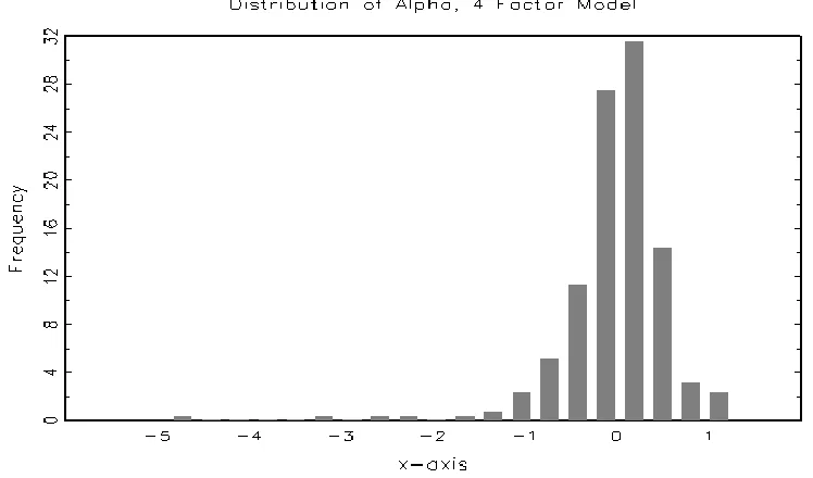
[Figure 3 here]
The distribution of alpha estimates (NAV returns) for the four-factor benchmark model shows a wide range of values (Figure 3). Most NAV-alphas are in the negative to 10.5% p.a. range but there are some funds in the extreme tails of the distribution which may have extremely ‘good’ or ‘bad’ security selection. This is important, since investors are more interested in holding funds in the right tail of the performance distribution and avoiding those in the extreme left tail, than they are in the average fund’s performance. This emphasizes the importance of examining fund-by-fund performance (rather than the weighted average of all funds) and then correcting for false discoveries to provide an assessment of overall industry performance.
Using NAV returns and the four-factor benchmark model (4FBM), we discuss estimates of the proportion of truly zero-alpha funds
0, positively skilled alpha-funds,
A and unskilled funds
A among our total of M-funds. We then analyze the false discovery rate for the positive-alpha and negative-positive-alpha funds taken separately; this allows us to ascertain whether such funds are concentrated in the tails of the performance distribution6.Estimation of
0The histogram of bootstrap p-values for the 4FBM when testing
H
0:
i
0
across funds is given in Figure 4. Exploiting the fact that truly null p-values are uniformly distributed [0, 1], the height of the flat portion of the histogram gives an estimate of the proportion of truly null-alpha funds
0. From Figure 4 a reasonable ‘eyeball’ estimate would be
= 0.2 giving
ˆ ( )
0 = 0.8.[Figure 4 here]
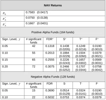
Taking the four-factor benchmark model (4FBM) and our universe of all M-funds, the MSE-bootstrap estimator gives the percentage of truly zero alpha funds
ˆ ( )
0 = 76% (se = 4.2), the percentage of negative-alpha funds
ˆ
A = 16.7% (se = 4.0) and skilled funds
ˆ
A= 7.5% (se = 1.4) – Table 3. It is the estimate of
ˆ ( )
0 which determines our FDR (for alpha) and this is statistically well determined because the estimation uses data on a large number of null funds. Standard errors are in parentheses and are given in Genovese and Wasserman 2004 (and Barras et al. 2010, Appendix A). Hence in the whole population of funds, most have truly zero alphas, but there is a small proportion of funds with statistically positive or negative alphas. We now examine the location of these non-zero alpha funds.As we increase the significance level
, the number of statistically significant positive alpha fundsS
(Table 3, Panel A) and negative alpha fundsS
(Table 3,Panel B) increases. However,FDR
andFDR
also increase so that the proportion of truly skilled fundsT
and truly unskilled fundsT
does not vary substantially with
. This implies that the skilled and unskilled funds lie predominantly in the extreme tails (i.e. for
0.05
), rather than being evenly spread throughout the tails.6As noted below, the results using different models to estimate 0
[Table 3 here]
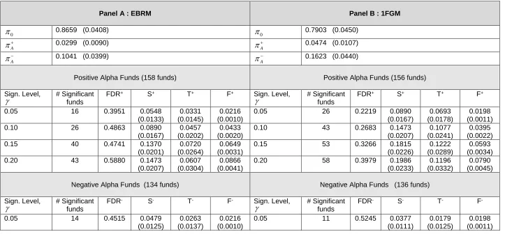
The histogram of p-values when testing
H
0:
i
0
for the excess benchmark return model (EBRM) and the one-factor benchmark model (1FBM) are similar to those for the four-factor benchmark model (4FBM) in Figure 4 (and are not presented here). This results in broadly similar values for
0 as for the 4FBM -
0is equal to 86.5% for ERBM and 79.0% for 1FBM (Table 4, Panels A and B).[Table 4 here]
Across the three models a salient feature is the resultant fall in
FDR
and the rise in the number of truly skilled fundsT
as we move from the Excess Return Benchmark Model (ERBM) to the one-factor benchmark model (1FBM in Table 4) and then to the four-factor benchmark model (4FBM in Table3). For example, for
=0.10 we haveFDR
equal to 48.3%, 26.8% and 20.1% andT
equal to 4.6% , 10.8% and 15.0% when moving from ERBM to 1FBM and to 4FBM respectively.Turning now to negative-alpha funds, we find that as we move from the Excess Return Benchmark Model (EBRM) to the one-factor benchmark model (1FBM in Table 4) and then to the four-factor benchmark model (4FBM in Table 3), the number of truly negative skilled funds (
=0.10) remains largely constant withT
= 4.9%, 2.6%, and 3.7% of the funds, respectively.The above results which use self-declared benchmarks are not a like-for-like comparison across funds and this might influence the cross-section of alphas7. As a robustness test we
therefore use a common global benchmark (in place of the self-declared benchmarks) but this does not appreciably alter the results in table 3. For example, if we take a significance level of
= 10% then the number of truly skilled funds isT
= 15% (se=2.6%) in table 3 (4FBM) andT
= 18.7% (se=2.7%) when using the common global benchmark (4FGM) - so the results are qualitatively similar. For unskilled funds we haveT
= 3.7% (se= 1.9%) in table 3 andT
= 0.9% (se= 1.6%) for the 4FGM – hence although the point estimates differ they are both statisticallyequal to zero. In addition, using the self-declared benchmarks gives an average
R
2of 66.6% (across all funds) while using the common global benchmark has an averageR
2 of 52.2%.Persistence in Portfolios of CEF
Using NAV returns, we have established that there is some positive and some negative manager skill in security selection (alpha) when holding individualfunds over the whole sample period. We now wish to examine whether forming portfolios by switching between different funds gives a positive-alpha performance in the post-formation period.
We form portfolios using a rolling window based on either the excess benchmark return model (EBRM) or on past t-alphas from the one-factor benchmark model (1FBM) – using NAV returns (ie. based on individual manager skill over the formation period). Our performance measure is based on fund-price returns in the post-formation period.8 We report results for
post-formation alphas using a post-formation period of
f
12
months and for alternative holding periods h = 12, 3, 1 months. Because the post-formation portfolios contain funds with different investment objectives, it is not possible to estimate a post-formation factor model which incorporates all the self-declared benchmarks. Hence, we use the one- and four-factor global models to assess the post-formation alphas (for fund-price returns).Post-formation decile-sorted portfolio alphas, together with their bootstrap p-values are reported for funds sorted by the excess benchmark return model (EBRM) in Table 5 and by the t-alpha of the one-factor benchmark model (1FBM) in Table 6. In each table, Panel A reports the results for the post-formation alphas of the one-factor global model (1FGM), Panel B reports those of the three-factor global model (3FGM) and Panel C those of the four-factor global model (4FGM).
[Table 5 here]
Funds Sorted using EBRM
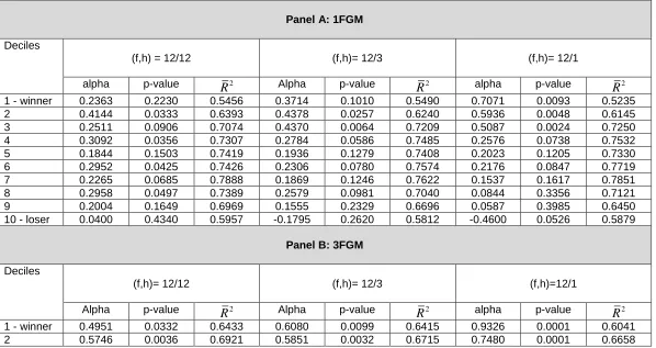
When we sort funds based on the excess benchmark return model (EBRM) and evaluate the post-formation alphas for fund-price returns using the one-factor benchmark model (1FBM in Table 5, Panel A), we find about 4 out of the 10 decile portfolios have statistically significant post-formation alphas (at a 5% significance level) but there is no clear pattern of past ‘winners’
8 It seems unlikely that (predominantly) retail investors would be concerned with an active strategy where the
remaining ‘winners’, except when we use
f h
,
(12,1)
when there is persistence in winner funds for deciles 1 to 3. When evaluating the post-formation alphas using the three-factor global model (3FGM in Panel B) or four-factor global model (4FGM in Panel C), we find more positive post-formation alphas for all deciles and for all three combinations of( , )
f h
.When moving from the one-factor global model (IFGM) to the four-factor global model (4FGM), the increase in the number of decile portfolios with statistically significant positive post-formation alphas is partly due to a reduction in residual variance (indicated by an increase in of around 10% for each decile portfolio) and also to an increase in the point estimates of post-formation alphas. With the standard errors of the alphas remaining largely constant, the latter leads to an increase in the statistical significance of the decile portfolio alphas.
[Table 6 here] Funds Sorted using t-alpha of 1FBM
The same pattern of results reported above, applies when funds are sorted on the t-alpha of the one-factor benchmark model (rather than EBRM) and evaluated using the global models (Table 6, Panels A, B, and C).
Irrespective of whether we form portfolios based on excess returns over fund-specific self-declared benchmarks EBRM (Table 5) or on the t-alphas of the one-factor benchmark model (Table 6), we obtain much stronger evidence of positive post-formation alphas, when using the four-factor global model (
r SMB HML MOM
m,
,
,
) rather than the one-factor global model (r
m). This applies for all three rebalancing periods h = 1,3, and 12 months.9 These results are incontrast to those reported for the UK and US open-end fund industry using a four-factor model where there is little evidence of positive post-formation alphas and much stronger evidence negative post-formation alphas.
Funds Sorted using t-alpha of 4FBM
As a further robustness test we take account of the fact that for closed-end funds, price-returns (to the investor) may exhibit greater momentum than for mutual funds – since the premium or discount may persist (and this is not reflected in NAV returns). We therefore form portfolios of funds based on the t-alpha of the 4FBM (ie. including a momentum variable) using price-returns and use the 4FGM (with price-returns) as in table 6, to measure the post-formation
9Recursive least squares analysis of the post-formation alphas reveals that it is only post-2001 that the alphas are
statistically significant.
2
performance. We again find a substantial number of positive-alpha decile portfolios in the post-formation period (table 7)10.
[Table 7 here]
Which performance model should we use? For the four-factor global model, all four factors in the post-formation regressions are statistically significant for all deciles and the ’s of 70%-75% suggest that these global factors capture most of the variability in fund-price portfolio returns. Whether the four-factor global model is the ‘correct’ model for closed-end funds could be debated but, for example, the four factors explain more of the variation in closed-end fund returns than do factor models applied to hedge fund returns – where positive alpha performance is also found. As both hedge funds and closed-end funds can hold heterogeneous portfolios and use leverage (whereas open-end funds cannot), this provides one possible reason for the positive post-formation alphas for closed-end funds.
5. Conclusion
We use the false discovery rate to assess the overall alpha-performance of UK closed-end funds using self-declared benchmarks and additional risk factors. We find evidence that around 16% of the funds in our sample have truly positive alphas (using a four-factor model that includes a self-designated benchmark or where the latter is replaced by a global benchmark). The number of truly negative alpha funds is around 1-4% of our sample of funds and is largely invariant to the factor model used. This is a better performance overall than UK and US open-end funds where around 0%-5% of the positive alpha funds and 25% of the negative alpha funds are found to be statistically significant.
Examining persistence in performance, we find that positive post-formation alpha fund performance depends on the factor model used – there is some positive-alpha performance when post-formation returns are evaluated using a one-factor global market model but substantial positive-alpha performance is found when using a four-factor global model. The magnitude of the alpha increases as global risk factors proposed by Fama-French (1993) and Carhart (1997) are included in our factor model. If we accept the four-factor global model, then decile portfolios of closed-end funds give rise to positive post-formation alphas and fund performance more
10 This variant was suggested by an anonymous referee. We also find qualitatively similar results when we form portfolios of funds based on the t-alpha of the four-factor global model 4FGM using price-returns (rather than the 4FBM) and also use the 4FGM (with price-returns) in the post-formation period (as in tables 6 and 7) - these results are available from the authors.
2
References
Alexander, G.J., Cici, G. and Gibson, S., 2007, Does Motivation Matter When Assessing Trade Performance? An Analysis of Mutual Funds, Review of Financial Studies, Vol. 20, No. 1, pp. 125-150
Bajgrowicz, Pierre and Olivier Scaillet 2012, Technical Trading Rules Revisited: False Discoveries, Persistence Tests, and Transaction Costs, Journal of Financial Economics, Vol. 106, No. 3, pp. 437-491
Bangassa, K., 1999, Performance of UK Investment Trusts, Journal of Business, Finance and Accountancy, Vol. 26, No. 9/10, pp. 1141-1168
Bangassa, K., Su, C. and Joseph, N.L., 2012, Selectivity and Timing Performance of UK Investment Trusts, Journal of International Financial Markets, Institutions and Money, Vol. 22, No. 5, pp. 1149-1175
Barras, Laurent, Olivier Scaillet, and Russ Wermers, 2010, False Discoveries in Mutual Fund Performance: Measuring Luck in Estimated Alphas, Journal of Finance, Vol. 65, No. 1, pp. 179-216.
Benjamini Y. and Y. Hochberg, 1995, Controlling the False Discovery Rate: A Practical and Powerful Approach to Multiple Testing, Journal of Royal Statistical Society, Vol. 57 (1), pp. 289-300.
Bers, M.K. and Madura, J., 2000, The Performance Persistence of Closed-End Funds, The Financial Review, Vol. 35, pp. 33-52
Bessler, Wolfgang, David Blake, Peter Luckoff and Ian Tonks, 2010, Why Does Mutual Fund Performance Not Persist? The Impact and Interaction of Fund Flows and Manager Changes, Pensions Institute, Cass Business School, WP PI-1009.
Blake, David, and Allan Timmermann, 1998, Mutual Fund Performance: Evidence from the UK, European Finance Review, 2, 57-77.
Capocci, D. and Hubner, G., 2004, Analysis of Hedge Fund Performance, Journal of Empirical Finance, Vol. 11, No. 1, pp. 55-89
Carhart, Mark M, 1997, On Persistence in Mutual Fund Performance, Journal of Finance Vol. 52, pp. 57-82
Chen, Joseph, Harrison Hong, Ming Huang and Jeffrey D. Kubik 2004, Does Fund Size Erode Mutual Fund Performance? The Role of Liquidity and Organization, American Economic Review, 94, 1276-1302.
Cherkes, M., Sagi, J. and Stanton, R., 2009, A Liquidity Based theory of Closed End Funds, Review of Financial Studies, 22, 257-97.
Coval, Joshua D. And Erik Stafford 2007, Asset Fire Sales (and Purchases) in Equity Markets, Journal of Financial Economics, 86, 479-512.
Criton, Gilles and Olivier Scaillet, 2011, Time-Varying Analysis in Risk and Hedge Fund Performance : How Forecast Ability Increase Estimated Alpha, SSRN Working Paper, March.
Funds: Luck or Skill ? “, Journal of Empirical Finance, Vol. 15(4), pp. 613-634. Cuthbertson, Keith, Dirk Nitzsche and Niall O’Sullivan, 2012, ‘False Discoveries in UK
Mutual Fund Performance“, European Financial Management, Vol. 18(3), pp. 444-463.
Dangl, Thomas, Youchang Wu and Josef Zechner, 2008, Market Discipline and Internal Governance in the Mutual Fund Industry, Review of Financial Studies, Vol. 21, No. 5, pp. 2307-2343.
Del Guercio, Diane and Paula A. Tkac, 2008, Star Power: The Effect of Morningstar Ratings on Mutual Fund Flow, Journal of Financial and Quantitative Analysis, Vol. 43, No. 4, pp. 907-936
Edelen, R.M., 1999, Investor Flows and the Assessed Performance of Open-end Mutual Funds, Journal of Financial Economics, Vol. 53, No. 3, pp. 439-466
Efron, B., and R.J. Tibshirani, 1993. An Introduction to the Bootstrap, Monographs on Statistics and Applied Probability (Chapman and Hall, New York).
Elton, E.J., Gruber, M., Blake, C.R. and Shachar, O., 2013, Why Do Closed-End Bond Funds Exist? : An Additional Explanation for the Growth in Domestic Closed-End Bond Funds, Journal of Financial and Quantitative Analysis, Vol. 48, No. 2, pp. 405-425.
Elton, Edwin J., Martin J. Gruber, Das, S. and Hlavka, M. 1993, Efficiency with Costly Information: A Reinterpretation of Evidence from Managed Portfolios, Review of Financial Studies, Vol. 6, pp. 1-21.
Elyasiani, E and Jia J., 2011, Performance Persistence of Closed-End Funds, Review of Quantitative Finance and Accounting, Vol. 37, pp. 381-408.
Fama, Eugene F. and Kenneth R. French, 1993, Common Risk Factors in the Returns on Stocks and Bonds, Journal of Financial Economics, Vol. 33, pp. 3-56.
Fama, Eugene F. and Kenneth R. French, 2010, Luck versus Skill in the Cross Section of Mutual Fund Returns, Journal of Finance, Vol. 65, No. 5, pp. 1915-1947. Fletcher, Jonathan, 1997, An Examination of UK Unit Trust Performance Within the
Arbitrage Pricing Framework, Review of Quantitative Finance and Accounting, Vol. 8, pp. 91-107.
Gemmill, Gordon and Dylan C. Thomas, 2002, Noise Trading, Costly Arbitrage and Asset Prices: Evidence from Closed-End Funds, Journal of Finance, Vol.57, pp. 2571-2594.
Genovese, C. and Wassermann, L. 2004, A Stochastic Process Approach to False Discovery Control, Annals of Statistics, Vol. 32, No. 3, pp. 1035-1061
Ivkovic, Zoran and Scott Weisbenner, 2009, Individual Investor Mutual Fund Flows, Journal of Financial Economics, 92, 223-237.
85-118.
Khorana, Ajay, 1996, Top Management Turnover: An Empirical Investigation of Mutual Fund Managers, Journal of Financial Economics, 40 (3), pp. 403-427.
Khorana, Ajay, 2001, Performance Changes Following Top Management Turnover: Evidence From Open-End Mutual Funds, Journal of Financial and Quantitative Analysis, 36, 371-393.
Kosowski, R., A. Timmermann, H. White and R. Wermers, 2006, Can Mutual Fund ‘Stars’ Really Pick Stocks? New Evidence from a Bootstrapping Analysis, Journal of Finance, Vol. 61, No. 6, pp. 2551-2595.
Lee C., Shleifer, A. and Thaler R, 1990, Anomalies: Closed-End Mutual funds, Journal of Economic Perspectives, Vol. 4, pp. 153-64.
Madura, J. and Bers, M.K, 2002, The Performance Persistence of Foreign Closed-End Funds’, Review of Financial Economics, Vol. 11, No. 4, pp. 263-285
Malkiel, G., 1995, Returns from Investing in Equity Mutual Funds 1971 to 1991, Journal of Finance, Vol. 50, pp. 549-572.
McCracken, Michael. W. and Stephen G. Sapp, 2005, Evaluating the Predictabililty of Exchange Rates Using Long-Horizon Regressions: Mind Your p’s and q’s, Journal of Money Credit and Banking, Vol. 37(3), pp. 473-494.
Politis, D.N. and J.P. Romano, 1994, The Stationary Bootstrap, Journal of the American Statistical Association, Vol. 89, pp. 1303-1313.
Pollet, J.M. and Wilson, M., 2008, How Does Size Affect Mutual Fund Behaviour?, Journal of Finance, Vol. 63, No. 6, pp. 2941-2969
Quigley, Garrett, and Rex A. Sinquefield, 2000, Performance of UK Equity Unit Trusts, Journal of Asset Management, Vol. 1, pp. 72-92
Sensoy, B.A., 2009, Performance Evaluation and Self-Designated Benchmark Indexes in the Mutual Fund Industry, Journal of Financial Economics, Vol. 92, No. 1, pp. 25-39.
Storey J. D., 2002, A Direct Approach to False Discovery Rates, Journal of Royal Statistical Society B, Vol. 64, pp. 497-498.
Storey, J. D., J.E. Taylor and D. Siegmund, 2004, Strong Control, Conservative Point Estimation and Simultaneous Conservative Consistency of False Discovery Rates: A Unified Approach, Journal of Royal Statistical Society, Vol. 66, pp. 187-205.
Wermers, R., 2000, Mutual Fund Performance: An Empirical Decomposition into Stock-Picking Talent, Style, Transaction Costs, and Expenses, Journal of Finance, Vol. 55, pp. 1655–95.
Figure 1
Recursive Alpha: Fund-Price Returns, Four-Factor Global Model (4FGM)
Figure 2
[image:23.612.103.504.437.685.2]Figure 3
Alpha Estimates: NAV Returns, Four-Factor Benchmark Model (4FBM)
Figure 4
Alpha p-values: NAV returns: Four-Factor Benchmark Model (4FBM)
Bootstrap p-values under
H
0:
i
0
for 292 funds with a minimum of 18 monthly observations over the period November 1990 to January 2013 for the four-factor model (4FBM), with NAV returns. The four-factor model (4FBM) includes the self-declared benchmark and global factors for size, book-to-market, and momentum.p-values of skilled and unskilled
funds
Area to the right are
p-values of zero alpha funds
Area under this line
0= [1/(1-
]{#p>
}/M = 0.76
Table 1 Summary Statistics
This table reports summary statistics for all funds with at least 18 monthly observations. The sample period is November 1990 to January 2013. There are 292 funds with an average of 154 monthly observations for NAV returns and 298 funds with an average of 152 monthly observations for fund-price returns. We report averages of the individual fund statistics for both NAV returns and fund-price returns using 3 models, The models are the excess benchmark return model (EBRM), the one-factor benchmark model (1FBM) and the four-factor benchmark model (4FBM) which includes the self-declared fund benchmark and global factors for size, book-to-market, and momentum). Newey-West heteroscedastic and autocorrelation adjusted standard errors are reported. The percentage of funds with non-normal residuals is based on the Bera-Jarque B-J statistic. Statistical significance is at the 5% significance level (two tail test).
Excess Benchmark Return Model EBRM One-Factor Benchmark Model 1FBM Four-Factor Benchmark Model 4FBM NAV- Returns Fund-Price Returns NAV- Returns Fund-Price Returns NAV- Returns Fund-Price Returns % statistically significant
positive alpha
5.82% 3.02% 8.90% 3.69% 14.73% 10.07% % statistically significant
negative alpha
5.48% 0% 4.79% 0.67% 4.79% 0.34% Alpha (stdv) -0.0723 (0.5505) -0.0056 (0.5920) -0.0374 (0.5411) 0.0302 (0.6063) -0.0115 (0.5739) 0.1275 (0.6281) Self-declared benchmark (stdv)
- - 0.8202 (0.2979) 0.8632 (0.3163) 0.8085 (0.2906) 0.8362 (0.3125) SMB (stdv)
- - - - 0.1760
(0.2858)
0.2503 (0.4091) HML
(stdv )
- - - - -0.0851
(0.3225)
-0.1145 (0.4336) MOM
(stdv)
- - - - -0.0288
(0.2219)
-0.1370 (0.3049) Mean
R
2 (%) N/A N/A 61.50 46.01 66.84 50.97 % funds, non-normalresiduals using B-J test
Table 2 Equally Weighted Portfolio of all CEF: Fund-Price and NAV Returns.
This table reports the estimated coefficients together with their t-statistics for the one-factor global model (1FGM) and the four-factor global model (4FGM) using an equally-weighted portfolio of all funds over the sample period January 1996 to December 2012. The 1FGM uses the excess return on a global stock market index. The 4FGM includes factors for the global stock market index and global size, book-to-market, and momentum variables. Figures in parentheses are t-statistics using Newey-West heteroscedastic and autocorrelation adjusted standard errors.
Panel A: 1FGM Alpha Market
Return
SMB HML MOM 2
R
(%) Fund-Price Returns 0.1588 (1.05) 0.9239 (16.91)- - - 74.30
NAV Returns 0.1087 (0.90) 0.8764 (25.68)
- - - 84.55
Panel B: 4FGM Alpha Market
Return
SMB HML MOM 2
Table 3 False Discovery Rate: NAV Returns, Four-Factor Benchmark Model (4FBM)
This table reports the false discovery rate statistics for NAV returns using the four-factor benchmark model (4FBM). The four factors are the self-declared benchmark and the global risk factors SMB, HML and MOM. The sample period is from November 1990 to January 2013 using 292 funds with at least 18 monthly observations. p-values under the null
0
are calculated based on 10,000 bootstrap simulations. Standard errors are in parentheses.NAV Returns
0
0.7583 (0.0417)A
0.0750 (0.0138)A
0.1667 (0.0401)Positive Alpha Funds (164 funds) Sign. Level,
# significantfunds
FDR+ S+ T+ F+
0.05 42 0.1318 0.1438 (0.0205)
0.1249 (0.0216)
0.0190 (0.0010) 0.10 55 0.2013 0.1884
(0.0229)
0.1504 (0.0260)
0.0379 (0.0021) 0.15 65 0.2555 0.2226
(0.0243)
0.1657 (0.0302)
0.0569 (0.0031) 0.20 72 0.3075 0.2466
(0.0252)
0.1707 (0.0344)
0.0758 (0.0042) Negative Alpha Funds (128 funds)
Sign. Level,
# significant fundsFDR- S- T- F
-0.05 15 0.3690 0.0514 (0.0129)
0.0324 (0.0141)
(0.0154) (0.0190) (0.0021) 0.15 32 0.5190 0.1096
(0.0183)
0.0527 (0.0247)
0.0569 (0.0031) 0.20 36 0.6151 0.1233
(0.0192)
0.0475 (0.0292)
Table 4 False Discovery Rate: NAV returns, Excess Benchmark Return Model (EBRM) and One-Factor Benchmark Model (1FBM)
This table reports the false discovery rate statistics for two models. Panel A reports the statistics for the Excess Benchmark Return Model (EBRM) and panel B for the one-factor benchmark model (1FBM). The sample period is from November 1990 to January 2013 using 292 funds with at least 18 monthly observations on NAV returns. The p-values under the null
0
are calculated based on 10,000 bootstrap simulations. Standard errors are in parentheses.Panel A : EBRM Panel B : 1FGM
0
0.8659 (0.0408)0
0.7903 (0.0450)A
0.0299 (0.0090)A
0.0474 (0.0107)A
0.1041 (0.0399)A
0.1623 (0.0440)Positive Alpha Funds (158 funds) Positive Alpha Funds (156 funds) Sign. Level,
# Significant funds
FDR+ S+ T+ F+ Sign. Level,
# Significant funds
FDR+ S+ T+ F+
0.05 16 0.3951 0.0548 (0.0133)
0.0331 (0.0145)
0.0216 (0.0010)
0.05 26 0.2219 0.0890 (0.0167)
0.0693 (0.0178)
0.0198 (0.0011) 0.10 26 0.4863 0.0890
(0.0167)
0.0457 (0.0202)
0.0433 (0.0020)
0.10 43 0.2683 0.1473 (0.0207)
0.1077 (0.0241)
0.0395 (0.0022) 0.15 40 0.4741 0.1370
(0.0201)
0.0720 (0.0264)
0.0649 (0.0031)
0.15 53 0.3266 0.1815 (0.0226)
0.1222 (0.0289)
0.0593 (0.0034) 0.20 43 0.5880 0.1473
(0.0207)
0.0607 (0.0304)
0.0866 (0.0041)
0.20 58 0.3979 0.1986 (0.0233)
0.1196 (0.0332)
0.0790 (0.0045) Negative Alpha Funds (134 funds) Negative Alpha Funds (136 funds)
Sign. Level,
# Significant funds
FDR- S- T- F- Sign. Level,
# Significant funds
FDR- S- T- F
-0.05 14 0.4515 0.0479 (0.0125)
0.0263 (0.0137)
0.0216 (0.0010)
0.05 11 0.5245 0.0377 (0.0111)
0.0179 (0.0125)
0.10 27 0.4683 0.0925 (0.0170)
0.0492 (0.0204)
0.0433 (0.0020)
0.10 19 0.6073 0.0651 (0.0144)
0.0256 (0.0184)
0.0395 (0.0022) 0.15 38 0.4991 0.1301
(0.0649)
0.0652 (0.0260)
0.0649 (0.0031)
0.15 29 0.5968 0.0993 (0.0175)
0.0400 (0.0245)
0.0593 (0.0034) 0.20 41 0.6167 0.1404
(0.0866)
0.0538 (0.0301)
0.0866 (0.0041)
0.20 43 0.5367 0.1473 (0.0207)
0.0682 (0.0310)
Table 5
Persistence in Alpha: Funds Sorted by Alpha using NAV Returns and the Excess Benchmark Return Model (EBRM)
Funds are sorted into past ‘winner’ and ‘loser’ deciles using NAV returns and the Excess Benchmark Returns Model. The table reports alphas (and bootstrap p-values) for post-formation fund-price returns using the one-factor global model (1FGM, Panel A), the three-factor global model (3FGM, Panel B) and the four-factor global model (4FGM, Panel C). The formation (f) and holding (h) periods (f,h) are 12/12, 12/6 and 12/1 months. The 1FGM uses the excess return on a global stock market index, the 3FGM also includes global factors for size and book-to-market; the 4FGM adds a momentum variable. The investment horizon is 17 years (204 months), starting in January 1996 and ending in December 2012.
Panel A: 1FGM Deciles
(f,h) = 12/12 (f,h)= 12/3 (f,h)= 12/1 alpha p-value 2
R
Alpha p-valueR
2 alpha p-valueR
21 - winner 0.2363 0.2230 0.5456 0.3714 0.1010 0.5490 0.7071 0.0093 0.5235 2 0.4144 0.0333 0.6393 0.4378 0.0257 0.6240 0.5936 0.0048 0.6145 3 0.2511 0.0906 0.7074 0.4370 0.0064 0.7209 0.5087 0.0024 0.7250 4 0.3092 0.0356 0.7307 0.2784 0.0586 0.7485 0.2576 0.0738 0.7532 5 0.1844 0.1503 0.7419 0.1936 0.1279 0.7408 0.2023 0.1205 0.7330 6 0.2952 0.0425 0.7426 0.2306 0.0780 0.7574 0.2176 0.0847 0.7719 7 0.2265 0.0685 0.7888 0.1869 0.1246 0.7622 0.1537 0.1617 0.7851 8 0.2958 0.0497 0.7389 0.2579 0.0981 0.7040 0.0844 0.3356 0.7121 9 0.2004 0.1649 0.6969 0.1555 0.2329 0.6696 0.0587 0.3985 0.6450 10 - loser 0.0400 0.4340 0.5957 -0.1795 0.2620 0.5812 -0.4600 0.0526 0.5879
Panel B: 3FGM Deciles
(f,h)= 12/12 (f,h)= 12/3 (f,h)=12/1 Alpha p-value 2
R
Alpha p-valueR
2 alpha p-valueR
23 0.3456 0.0262 0.7317 0.5142 0.0011 0.7397 0.6149 0.0002 0.7565 4 0.3834 0.0141 0.7458 0.3759 0.0150 0.7684 0.3586 0.0167 .0.7756 5 0.2785 0.0519 0.7616 0.2840 0.0412 0.7606 0.2932 0.0383 0.7528 6 0.3422 0.0226 0.7478 0.2639 0.0521 0.7611 0.2604 0.0504 0.7764 7 0.2315 0.0657 0.7948 0.2331 0.0774 0.7712 0.1954 0.1109 0.7892 8 0.3500 0.0282 0.7477 0.3221 0.0486 0.7156 0.1125 0.2881 0.7199 9 0.2566 0.1003 0.7034 0.2246 0.1417 0.6792 0.1295 0.2747 0.6565 10 - loser 0.1786 0.2397 0.6265 -0.0471 0.4362 0.6065 -0.3240 0.1261 0.6156
Panel C: 4FGM Deciles
(f,h) = 12/12 (f,h)= 12/3 (f,h)=12/1 Alpha p-value 2
R
Alpha p-valueR
2 alpha p-valueR
2Table 6 Persistence in Alpha: Funds Sorted by t-alpha using NAV Returns and the One-Factor Benchmark Model (1FBM)
Funds are sorted into past ‘winner’ and ‘loser’ deciles using NAV returns and the one-factor benchmark model (1FBM). The table reports alphas (and bootstrap p-values) for post-formation fund-price returns using the one-factor global model (1FGM, Panel A), the three-factor global model (3FGM, Panel B) and the four-factor global model (4FGM, Panel C). The formation (f) and holding (h) periods (f,h) are 12/12, 12/6 and 12/1 months. The 1FGM uses the excess return on a global stock market index, the 3FGM also includes global factors for size and book-to-market; the 4FGM adds a momentum variable. The investment horizon is 17 years (204 months), starting in January 1996 and ending in December 2012.
Panel A: 1FGM Deciles
(f,h) = 36/12 (f,h) = 36/3 (f,h) = 36/1 Alpha p-value 2
R
Alpha p-valueR
2 Alpha p-valueR
21 - winner 0.3505 0.0573 0.6453 0.4652 0.0197 0.6180 0.6007 0.0027 0.6327 2 0.3676 0.0435 0.6604 0.4633 0.0111 0.7040 0.5735 0.0008 0.7221 3 0.1157 0.2832 0.7136 0.1856 0.1570 0.7520 0.2920 0.0565 0.7504 4 0.4123 0.0154 0.7237 0.3344 0.0454 0.7090 0.3944 0.0261 0.7226 5 0.2462 0.0933 0.7333 0.3589 0.0255 0.7434 0.1998 0.1544 0.7116 6 0.2365 0.1068 0.7330 0.1128 0.2818 0.7305 0.2672 0.0716 0.7349 7 0.1856 0.1556 0.7170 0.2899 0.0511 0.7329 0.1298 0.2174 0.7518 8 0.3578 0.0272 0.7467 0.0296 0.4428 0.7027 0.1333 0.2661 0.6617 9 0.3222 0.0491 0.7058 0.2287 0.1195 0.6909 0.0527 0.3911 0.7025 10 - loser 0.2227 0.1474 0.6621 0.2726 0.1133 0.6545 0.0817 0.3571 0.6429
Panel B: 3FGM Deciles
(f,h) = 36/12 (f,h) = 36/3 (f,h) = 36/1 alpha p-value 2
R
Alpha p-valueR
2 Alpha p-valueR
24 0.5061 0.0028 0.7430 .0.4446 0.0097 0.7352 0.5247 0.0019 0.7560 5 0.3268 0.0303 0.7515 0.4182 0.0102 0.7550 0.2560 0.0932 0.7227 6 0.2934 0.0568 0.7406 0.1602 0.1931 0.7351 0.3259 0.0335 0.7422 7 0.2225 0.1171 0.7204 0.3602 0.0202 0.7440 0.1806 0.1425 0.7580 8 0.4141 0.0114 0.7535 0.0878 0.3252 0.7096 0.1976 0.1722 0.6703 9 0.3679 0.0285 0.7124 0.2904 0.0648 0.7016 0.1256 0.2516 0.7139 10 - loser 0.2962 0.0781 0.6752 0.3467 0.0599 0.6667 0.1361 0.2757 0.6543
Panel C: 4FGM Deciles
(f,h) = 36/12 (f,h) = 36/3 (f,h) = 36/1 alpha p-value 2
R
Alpha p-valueR
2 Alpha p-valueR
2Table 7 Persistence in Alpha: Funds Sorted by t-alpha using Fund-Price Returns and the Four-Factor Benchmark Model (4FBM)
Funds are sorted into past ‘winner’ and ‘loser’ deciles using fund-price returns and the four-factor benchmark model (4FBM). The four factors are the self-declared benchmark and the global risk factors SMB, HML and MOM. The table reports alphas (and bootstrap p-values) for post-formation fund-price returns using the four-factor global model (4FGM). The post-formation (f) and holding (h) periods (f,h) are 12/12, 12/6 and 12/1 months. The 4FGM uses the excess return on a global stock market index, global factors for size, book-to-market and momentum. The investment horizon is 17 years (204 months), starting in January 1996 and ending in December 2012.
Deciles
(f,h) = 36/12 (f,h) = 36/3 (f,h) = 36/1 Alpha p-value 2