Estimating Worst Case Failure Dependency with Partial Knowledge of the Difficulty Function

City, University of London Institutional Repository

Citation

:

Bishop, P. G. & Strigini, L. (2014). Estimating Worst Case Failure Dependency

with Partial Knowledge of the Difficulty Function. Paper presented at the 33rd International

Conference, SAFECOMP 2014, 10-09-2014 - 12-09-2014, Florence, Italy.

This is the accepted version of the paper.

This version of the publication may differ from the final published

version.

Permanent repository link:

http://openaccess.city.ac.uk/12850/

Link to published version

:

http://dx.doi.org/10.1007/978-3-319-10506-1

Copyright and reuse:

City Research Online aims to make research

outputs of City, University of London available to a wider audience.

Copyright and Moral Rights remain with the author(s) and/or copyright

holders. URLs from City Research Online may be freely distributed and

linked to.

knowledge of the difficulty function

Peter Bishop1,2 and Lorenzo Strigini1

1

Centre for Software Reliability, City University, London, UK

{pgb,strigini}@csr.city.ac.uk

2

Adelard LLP, London, Exmouth House, London, UK

[email protected]

Abstract—For systems using software diversity, well-established theories show that the expected probability of failure on demand (pfd) for two diverse program versions failing together will generally differ from what it would be if they failed independently. This is explained in terms of a “difficulty function” that varies between demands on the system. This theory gives insight, but no specific prediction unless we have some means to quantify the difficulty func-tion. This paper presents a theory leading to a worst case measure of “average failure dependency” between diverse software, given only partial knowledge of the difficulty function. It also discusses the possibility of estimating the model parameters, with one approach based on an empirical analysis of previous sys-tems implemented as logic networks, to support pre-development estimates of expected gain from diversity. The approach is illustrated using a realistic safety system example.

Keywords. safety, software reliability, fault tolerance, failure dependency, software diversity, difficulty function.

1

Introduction

Software diversity has been advocated as a means of improving the reliability of safe-ty related software and in particular safesafe-ty systems that react to a demand, where a 1 out of 2 or a 2 out of 3 voting scheme can be used to ensure that some safety action is performed. This approach is used in industry (e.g. for railway interlocking), but de-velopment and maintenance is costlier than for a non-diverse system and it is not easy to predict in advance the likely safety improvement that can be achieved.

programs, the expected pfd for common failures of a diverse pair can also be less than the product of the expected pfds of the single versions.

To quantify via these theories the improvement in expected pfd for a diverse safety system, one would need to specify both the difficulty for every demand, and the de-mand profile. Difficulty functions will normally be impossible to estimate for real projects (although a posteriori difficulty estimates have been obtained [1, 15] for some “toy” applications where many different versions were developed [12]). In addi-tion, if the safety system is used in different operational contexts, the demand profile might also be different and this can change the expected pfds.

In this paper we examine an approach for a more modest, but still useful, goal of estimating the worst case improvement in average pfd, by deriving a worst case de-mand profile that only requires knowledge about two points on the difficulty function rather that characterizing the whole function.

The paper will first summarize the theory underlying the difficulty function, then identify the worst demand profile that maximizes the expected pfd for a pair of di-verse programs, relative to the expected pfd of a single version for a given difficulty function. We then consider what estimates for the expected pfd can be derived given different types of knowledge about the difficulty function. We also discuss means, and difficulties, for estimating the model parameters and tentatively suggest an ap-proach for systems implemented as logic networks.

2

The difficulty function

In these models, the process that delivers a program, with its unknown faults (if any), is modelled as the random sampling of a program from a “population of all pos-sible programs”. The (unknown) probability of “drawing” each specific pospos-sible pro-gram depends on the specification, the development process, the development team, etc. Given these factors, the “difficulty function” θ(x) is defined as the probability that such a “randomly drawn” program will fail on a given demand x.

The mean pfds of a single program (pfd1) and of common failure for a pair of

di-verse programs (pfd2) depend on the difficulty function θ(x) and the demand profile

p(x). For a difficulty function θ(x), the expected pfd of a single program version is:

pfd1 = ∑θ(x) p(x) (1)

We consider the case in which the two versions for a 1-out-of-2 system are devel-oped from the same process for the same specification: the two developments have the same “difficulty function” (Eckhardt and Lee model [4]). Thus pfd1 is the same for

both programs; among all the scenarios where this holds, this scenario, of identical difficulty functions, yields the highest (i.e., the worst) value of pfd2.

Assuming conditional independence between failures of the versions for each de-mand [4] (i.e., the two developments are independent [11]), the expected pfd for a randomly drawn pair of programs is then:

pfd2 increases with the variance of the difficulty function θ(x). Intuitively, if the

difficulty function is very “spiky”, there is a high probability that the diverse pro-grams will fail on the same, “difficult” demands: the average benefit from diverse programs will be lower than otherwise. Conversely if the difficulty function is “flat” (the same value for all demands), there is nothing that forces the diverse programs to fail on similar inputs, so the gain in average reliability is higher. In this case, pfd2 does

equal the product between the expected pfd values for the two versions. For brevity, when this equality holds we will say there is “independence on average”1.

Clearly the mean pfd depends upon the demand profile p(x) as well as the demand difficulty θ(x). In the next section we use this dependence on the demand profile to derive the worst case value of pfd2 for a given value of pfd1.

3

Estimating the worst case expected pfd

We compare the expected pfd for this system with that of a single-version (i.e., non-diverse) system used in the same function (hence with the same demand profile).

To determine the worst-case impact of the profile on the expected pfd, we choose the family of the most extreme profiles possible: the ones in which the only demand values with non-zero probabilities are x=hi and x=lo that have the highest and lowest values of the difficulty function, θ(hi) and θ(lo). For this profile, we can write:

pfd1 = zθ(hi) + (1−z)θ(lo) (3)

pfd2 = zθ(hi)2 + (1−z)θ(lo)2 (4)

where z = p(lo) and (1−z) = p(hi). So pfd1 and pfd2 can vary between their

mini-mum and maximini-mum values depending on z, i.e.:

min(pfd2) = θ(lo) 2 , z= 0 (5)

max(pfd2) =θ(hi) 2 , z = 1 (6)

No other profile can achieve this range, as non-zero probabilities for demands with intermediate θ values would reduce the maximum and increase the minimum value achievable. There is also another sense in which these profiles are “extreme”. Given a certain difficulty function, a given value of pfd1 can in general be the result of many

different profiles, only one of which is “extreme”2. This “extreme” profile is the one

1

We underscore that “independence on average” is a property of expected values, not of individual program pairs. If independence of failures held for every pair of diverse pro-grams, “independence on average” would also hold. However, “independence on average” could hold even if independence does not hold within each pair; and we can have pfd2 >pfd12

even in a population of pairs in which pairs with negative or zero correlation between fail-ures of their component versions are more common than pairs with positive correlation [10].

2

where pfd2 is largest, i.e., the advantage of diversity is smallest. Under this profile, the

expected pfd of a diverse pair, pfd2, is a linear combination of θ(lo) 2

and θ(hi)2 and hence a linear combination of (min pfd1)

2

and (max pfd1) 2

. This can be compared with the “best case” profile that only selects demands x with exactly the same difficulty, i.e. where θ(x)=pfd1, so from (2) that pfd2=pfd12 which represents “independence on

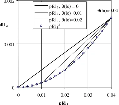
average”.. The expected pfds for the best and worst profiles are shown in Fig. 1 below

for the case where θ(hi)=0.04, and θ(lo) takes different values from zero to 0.02.

0 0.001 0.002

0 0.01 0.02 0.03 0.04 pfd 1

pfd 2

pfd 2 , θ(lo) = 0

pfd 2 , θ(lo)=0.01

pfd 2 , θ(lo)=0.02

pfd 12

θ(hi)=0.04

Fig. 1. Variation in pfd2, given the extreme profile and θ(hi)=0.04

To understand this graph, we consider that for a given value of θ(lo), the lowest possible value of pfd1 is θ(lo), given by setting z=0 in equation (3), and the

corre-sponding value of pfd2 equals θ(lo)2 (equation 4). This is why the straight lines for

θ(lo)=0.01 and θ(lo)=0.02 do not continue to the left of these points. The maximum values of pfd1 and pfd2 are given by setting z=1, and correspond to the rightmost point

in the graph, pfd1=θ(hi), pfd2=θ(hi)2. All the intermediate “extreme” profiles for the

same values of θ(lo) and θ(hi) give the {pfd1, pfd2} pairs represented by the points of

the straight line joining these maximum and minimum points on the pfd12 curve.

We now study the effects of various levels of knowledge about θ(hi) and θ(lo).

3.1 Case where

θ

(

)

θ

(

)

When

θ

(

)

θ

(

) are

)

(

)

(

)

(

lo

hi

pfd

hi

z

θ

θ

θ

−

−

=

)

(

)

(

)

(

1

lo

hi

lo

pfd

z

θ

θ

−

θ

−

=

−

)

(

)

(

))

(

)(

)

(

)

(

(

)

(

2 2

2 2

lo

hi

lo

pfd

lo

hi

lo

pfd

θ

θ

θ

θ

θ

θ

−

−

−

+

=

We note that if pfd1=θ(lo) or pfd1=θ(hi), then pfd2 = pfd1 2

. This is not surprising: these cases select profiles where all points have the same difficulty value: effectively a flat difficulty function, which is known to imply “independence on average”. It also follows that the reduction factor pfd2/pfd1 will vary between θ(lo) and θ(hi).

3.2 Case where only

θ

(

)

If θ(lo) is unknown, then the worst case assumption is that θ(lo) = 0, and hence equation (7) reduces to the following, known bound on pfd2:

1 2

(

hi

)

pfd

pfd

≤

θ

3.3 Case where

θ

(

)

θ

(

)

The worst case assumption is now θ(lo) = 0, θ(hi) = 1 and hence equation (8) re-duces to the extreme case where the bound is:

1 2

pfd

pfd

≤

In this case, the mean pfd of a diverse pair could be no better than that for a single version. The worst case – the equality in (9) holds – would mean that the programs developed have fail on some specific demands and no others (with probability 1). Comparison with the previous cases highlights how knowledge about the difficulty function allows us to reduce the mean value of pfd2 as a proportion of pfd1.

3.4 Case where the ratio between

θ

(

)

θ

(

)

In this case we only know the maximum “roughness” of the difficulty function, k, the ratio of θ(hi) to θ(lo), but not the absolute difficulty values. Hence

)

(

)

(

lo

hi

k

θ

θ

=

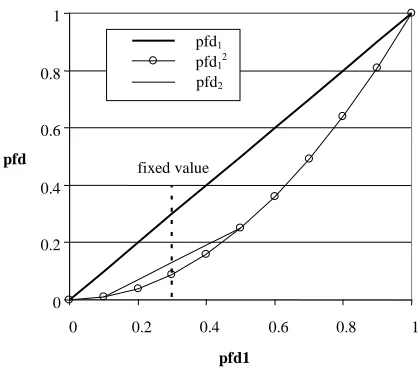
In this model, there is no constraint on the x axis endpoints θ(hi) and θ(lo) apart from the ratio k (and the fact that 0≤θ(lo)≤pfd1≤θ(hi)≤1). The worst case value of pfd2

Fig. 2. Worst case given a known difficulty ratio k

To get the worst case for a given pfd1, we effectively slide the linear combination

chord for pfd2 along the pfd12 curve, while keeping the ratio between the endpoints of

the chord (on the pfd1 axis) equal to k. Then we choose the chord that gives maximum

(worst) possible value of pfd2 for a given value of pfd1. Since pfd1 is held constant,

maximizing the ratio pfd2/pfd1 also maximizes pfd2/pfd12 (the worst case increase

relative to independence on average). The analysis in Appendix A shows that pfd2 is

bounded by:

2 1 2

2

4

)

1

(

pfd

k

k

pfd

≤

+

So the worst case reduction factor for pfd2 relative to pfd1 is pfd1⋅(k+1)2/4k, rather

than the factor of pfd1 that would result from “independence on average”.

This worst case bound equation is only applicable up to the point where θ(hi)=1 (as we cannot slide the pfd2 chord any further to the right). From the analysis in

Appen-dix A, it can be shown that this limit is reached when:

1

2

1

+

≥

k

pfd

If pfd1 exceeds this constraint, a variant of equation (7) has to be used instead

where θ(hi)=1 and θ(lo)=1/k, i.e.:

1 1 1 2 2

2

1

)

)(

1

(

− − −

−

−

−

−

+

=

k

k

pfd

k

k

pfd

1

2

1

+

≥

k

pfd

0 0.2 0.4 0.6 0.8 1

0 0.2 0.4 0.6 0.8 1

pfd1 pfd

pfd1 pfd12 pfd2

The difficulty “roughness” parameter, k, could be a very large value or even infin-ity if θ(lo)=0. Thus to forecast a good (low) worst-case pfd2 we need θ(hi) to be not

too high; counter-intuitively, we also need θ(lo) not to be too low: we need evidence that the probability of faults affecting any one demand will be “bad enough”.

4

Numerical illustration

For some non-realistic programs, we have empirical difficulty data derived from an analysis of program versions from an archive of mathematical problems and solutions [12]. Analysis of a population of around 3000 initial releases of program versions for a relatively simple problem [1] yielded the difficulty surface (taking the observed frequencies as estimates of probabilities) shown in Fig. 3 below.

0 60

120 180

-100-80-60-40-200

20 40 60801000 0.05 0.1 0.15

0.2 0.25

θ

t

v

Fig. 3. Empirical difficulty function from around 3000 program versions [1]. These programs receive two inputs, t and v, hence the difficulty function is plotted as a surface.

Analysis showed that θ(hi)=0.2282 and θ(lo)=0.1012. That is, in this case k = 0.2282/0.1012 = 2.25.

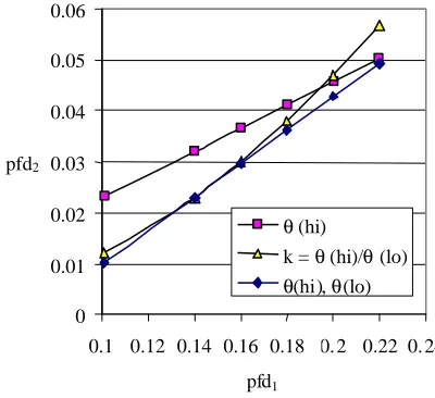
Inserting these values into equations 7, 8 and 9, the relationship between these bounding equations is illustrated in Fig. 4.

The bound based on knowledge of both θ(hi) and θ(lo) (equation 7) represents the least pessimistic worst case bound on pfd2. It can be seen that the curve based on an

estimate of k (equation 9) touches the least conservative bound line at the maximum dependency point when pfd1 = 0.140 (see Appendix A for details). Unlike equation 7,

equation 9 allows the maximum dependency point that defines pfd2 to be shifted if a

new estimate of pfd1 is made. This is equivalent to defining new values for θ(hi) and

θ(lo) which retain the same ratio k.

The pfd2 bound based on θ(hi) alone (equation 8) tends to be the most pessimistic,

(0.2282) when equations 7 and 8 agree with the “independence on average” result when pfd2 = pfd1

2

= θ(hi)2.

0 0.01 0.02 0.03 0.04 0.05 0.06

0.1 0.12 0.14 0.16 0.18 0. 2 0.22 0. 24 pfd1

pfd2

θ (hi)

k = θ (hi)/θ (lo)

θ(hi), θ(lo)

Fig. 4. Comparison of worst case bound equations. The labels for the three plots indicate which parameters are assumed known, with the values derived a posteriori for the study in Fig. 3.

5

Parameter estimation

In the analysis above we have identified alternative ways of deriving a worst case value for pfd2 given pfd1 by using different kinds of information about the difficulty

function. To apply these models for prediction, as opposed to generic insight, we require realistic model parameters. At the current state of knowledge, there are no means for deriving credible difficulty values to support prediction (estimation of ex-pected pfd) for a specific safety application. In the following subsections we examine some potential directions for deriving model parameters, and difficulties to be over-come for them to beover-come applicable in the future.

5.1 Estimating k

Estimation of k could be based on relative complexity, if one assumed the demand difficulty for demand x proportional to some measure of demand logic complexity3,

)

(

)

(

x

∝

c

x

θ

3

where c(x) is a measure of the logic complexity required to process a given demand x. For example, the complexity measure could based on the number of lines of code or number of decision points in the code involved in a particular type of demand. Program analysis (such as code pruning) could be used to identify the relevant subset of code involved with each demand. Assuming such complexity measures can be derived, k would be estimated as:

)

(

min

)

(

max

)

(

min

)

(

max

x

c

x

c

x

x

k

X x

X x

X x

X x

∈ ∈

∈

∈

_≈

=

θ

θ

This approach need not be restricted to conventional code. Many safety systems are represented as logic networks with a set of interconnected logic gates. Each type of demand requires different logic and sensor inputs to respond to different safety-related incidents on the associated plant. The complexity of the logic network could be used to estimate c(x).

5.2 Estimating θ(hi) and θ(lo)

One means of estimating θ(hi) is to make use of the fact that, by definition:

θ(hi) ≤pfaulty (16)

where pfaulty is the probability that a program selected from the population of all

possible program versions is faulty. The value of pfaulty could be estimated via a range

of methods including an analysis of the development process [2] and the level of test coverage achieved [9], however they are not mature methods and confidence in their predictions will be especially low when few faults are expected to be present.

Alternatively, estimates of θ(x) could be made directly based on some expected fault density f [13] and an estimate of the amount of code or logic n(x) needed to re-spond to a particular demand. There can be many demands x that exercise the same logic, but if we make a (strong) assumption that all demands are equally likely to fail if the logic is faulty (on average over the whole population), then:

θ(x) =n(x)f (17)

So the maximum and minimum values of n(x) over all types of demand x can be used to obtain θ(hi) and θ(lo).

5.3 Empirical data analysis

gas and electrical industrial sectors (but predominantly nuclear). A full set of data was collected for 125 PLCs which included the number of:

• inputs

• outputs

• coils

• failures

• years of use

No PLC “platform” failures were recorded in over 600 PLC-years of operation, suggesting that PLC platforms are fairly reliable. We should also note that “coils” were used as the measure of the number of logic elements, but we cannot be sure the actual logic network contained coils or whether an “equivalent coils” estimate was calculated for alternative types of logic. In addition, the term “failures” in this data set might actually be a misnomer for “number of faults”, as the failure counts are typi-cally zero or one. We assumed “failures” indicate the number of different faults. This is conservative from the viewpoint of estimating maximum difficulty as it can only over-estimate the number of network logic faults. Furthermore, if over-estimation of faults were consistent, it would not affect the k ratio derived in Section 3.4.

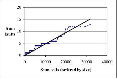
On further analysis, we found that some of the PLCs contained identical logic net-work metrics and identical fault counts. This was interpreted to mean that the same logic network was installed on multiple PLCs, which could bias the result by counting the same logic network several times over. These duplicates were eliminated from the analysis, leaving size and fault data for 96 different PLC programs. The results are presented in Fig. 5 below.

0 5 10 15 20

0 10000 20000 30000 40000 S um coils (ordered by size)

S um faults

Fig. 5. Logic faults vs. network coils (cumulative)

relation-ship does appear to be roughly linear (to 95% in a chi-squared test). Perhaps surpris-ingly, the slope seems to be slightly less for the larger PLC programs (at the right hand side of the graph).

A very similar graph was obtained when we used the sum of inputs and outputs (io) as the network size measure. Again, the correlation is better than 95% in a chi-squared test.

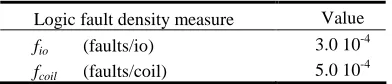
Given the evidence of a linear relationship between network size and logic faults, it may be legitimate to use an average fault density to estimate the number of faults in a logic network. The logic density estimates derived from the linear regression analysis of faults against the coil and io measures are shown in Table 1 below.

Table 1. Logic fault density estimates

Logic fault density measure Value

fio (faults/io) 3.0 10

-4 fcoil (faults/coil) 5.0 10

-4

Some caveats need to be placed on these fault density estimates, notably:

• The fault density is based on the number of fault discovered which could be an underestimate if some of the faults have yet to be found. The data in [14] shows the mean operating time is 5.9 years. It is not certain that all defects would have been detected over that period of time.

• Given the sparseness of failure data it cannot be demonstrated that linearity applies over the whole range of complexity. If the density is lower for small logic subsys-tems, k would be larger than predicted under the linearity assumption.

• We do not know which of the PLC faults were caused by errors in user require-ments or implementation. Common user requirement flaws cannot be mitigated by diverse logic implementations. Section 6 provides an example where we assume the fault density estimates relate to diverse implementation faults.

• Fault density figures will differ depending on the application type and safety criti-cality.

So the empirically derived figures might be viewed as indicative “ball-park” fig-ures, but should not be viewed as being applicable to a specific diverse system.

6

Example application

The application of the fault density quantification approach outlined in Section 5 is illustrated on an actual industrial safety system with two independent safety trains that control functionally diverse plant shutdown mechanisms4. The A and B train subsys-tems and logic element counts (taken from the logic specification sheets) are shown in Table 2 below.

4

Table 2. A and B Train subsystem network complexity measures

A Train subsystem I/O Gates

A1 24 16

A2 22 9

A3 49 28

A4 31 23

Total 126 76

B Train subsystem I/O Gates

B1 17 9

B2 28 16

B3 15 7

Total 60 32

We will use the data to illustrate the mean pfd estimation approach, using arbitrary (and quite extreme) assumptions about the variation of logic use with demands. Let us assume some logic subsystems are unnecessary for some demands. For example a standby electrical supply subsystem might be essential if connection to the grid power supply is lost but not otherwise.

So the extreme level of variation in number of subsystems with demand might be:

• One (the smallest) logic subsystem in A and B

• All logic subsystems in A and B

Using the io complexity measure we set an upper bound on the difficulty for a log-ic sub-network x containing nio(x) io elements as:

θ(x) = fio nio(x)

Based on the nio(x) numbers assumed for the assumed maximum and minimum

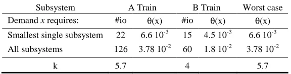
logic networks needed for a demand we derive the bounding values for θ and k shown in Table 3 below. Note that, in this particular example, the specified logic differs be-tween trains A and B, so we are assuming that there are no common specification flaws and the difficulty values estimate the likelihood of implementation flaws only.

Table 3. A and B Train difficulty and difficulty variation estimates

Subsystem A Train B Train Worst case Demand x requires: #io θ(x) #io θ(x) θ(x) Smallest single subsystem 22 6.6 10-3 15 4.5 10-3 6.6 10-3 All subsystems 126 3.78 10-2 60 1.8 10-2 3.78 10-2

k 5.7 4 5.7

For the A and B trains, different logic is involved, so the values are not identical, but we conservatively assume the worst case value applies to both trains. In the following calculation, we assume that the expected value pfd1 is 10-2for each train. This is

Table 3 above to yield the bounds on the expected value of pfd2 shown in Table 4

below.

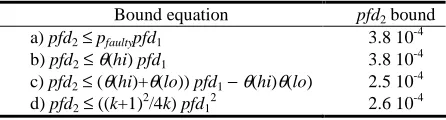
Table 4. Worst case A and B Train pfd estimates

Bound equation pfd2 bound

a) pfd2≤ pfaultypfd1 3.8 10-4

b) pfd2≤θ(hi) pfd1 3.8 10-4

c) pfd2≤ (θ(hi)+θ(lo)) pfd1−θ(hi)θ(lo) 2.5 10 -4

d) pfd2≤ ((k+1)2/4k) pfd12 2.6 10-4

It can be seen that in this example the results are very similar. The results for a) and b) are identical because the θ(hi) estimate is based on all the logic in the train and hence is identical to pfaulty for the train. The results for c) and d) are also similar since

the pfd1 value chosen is close to the maximum dependency point.

7

Discussion

It should be noted that the analysis in this paper relates to expected values. The analysis seeks to estimate the improvement we might expect between the averages pfd1 and pfd2 by using diversity, under worst case assumptions about the operational

profile. It does not predict the improvement ratio that will actually be achieved by a specific pair of program versions under a specific operational profile—clearly the actual reduction achieved could be better or worse than a model based on averages [10].

It is also important to note that this analysis describes the effects of those parts of development that are indeed diverse. For example, if there is a common specification, the possibility of a specification flaw would invalidate the conditional independence assumption required in the Eckhardt and Lee model [4]. Accounting for such common factors requires more complex models [11] and we have not checked how the ap-proach would extend to those models.

The paper also explores possible directions for quantifying the model parameters. The analysis of PLC failure data in Section 5 illustrates how one might attempt to estimate ranges of difficulty. However the method discussed should be viewed as “work in progress”, as it has not been validated or substantiated. In particular:

• It assumes that difficulty can be estimated from predicted fault density. This is not supported by deduction and could only be validated experimentally.

• There is an assumption of linearity between logic complexity and logic faults. This is not contradicted by the available empirical data but it would require far more empirical data to validate the assumption over the whole range of complexity.

Clearly further empirical studies are needed to check the underlying assumptions and to derive realistic faults density values before the models can be applied to high criticality systems. For validating this approach to estimating the difficulty function, the main obstacle is that direct empirical assessment of difficulty functions means counting faults affecting each demand in a large population of programs developed independently for the same specification. The rarity of such populations, outside labo-ratory experiments on toy problems, is the usual problem in empirical software engi-neering. Given instead sets of realistic, but practically unique programs, a feasible form of weaker validation would be to select sets of programs that are assessed to have the same parameters for the estimation method used, and then, within such a set of programs, measure fault frequencies over sets of demands estimated to have the same difficulty.

More generally, the current models assume a common difficulty function and fur-ther work is needed to generalize this approach to the case where the difficulty func-tions differ for the two versions (the Littlewood and Miller model [8]).

We also note that these bounding methods also apply to the models by Hughes [6] that explain correlation between random failures in redundant hardware in terms of variation of failure rates with environmental stress. Variation of failure rates with environmental factors will typically be easier to assess than variation of difficulty between demands.

8

Conclusions

We have developed models for estimating the worst case reduction in mean pfd achievable by diverse program pairs that require only a partial knowledge of the diffi-culty function. These models can give qualitative insight, e.g. about the effects of development decisions thought to increase or to reduce maximum or minimum diffi-culty. We have also discussed ways for estimating the parameters required for these models, and their difficulties; in particular, an approach for estimating difficulty val-ues and difficulty variation for applications defined in terms of a logic diagram.

We note that the methods discussed for deriving the difficulty parameters are very preliminary. Much more empirical support, especially for the high criticality systems where diversity is likely to be employed, would be needed before they could be ap-plied for quantitative prediction (e.g. for pre-development decisions about diversity). Further work is also needed to generalize the theory to cases where the difficulty functions differ for the diverse program versions.

References

1. Bentley, J.G.W., Bishop, P.G., van der Meulen, M.J.P.: An Empirical Exploration of the Difficulty Function. In: Computer Safety, Reliability, and Security (SAFECOMP) 2004, pp. 60-71, Springer (2004)

3. Eckhardt, D.E. and Caglayan, A.K., et al.: An experimental evaluation of software redun-dancy as a strategy for improving reliability. IEEE Trans Software Eng 17(7), 692-702 (1991)

4. Eckhardt, D.E., Lee, L.D.: A theoretical basis for the analysis of multiversion software subject to coincident errors. IEEE Transactions on Software Engineering 11(12), 1511-1517 (1985)

5. Hatton, L.: Reexamining the fault density-component size connection. IEEE Software, 14(2), 89-97 (1997)

6. Hughes, R.P.: A New Approach to Common Cause Failure. Reliability Engineering 17(3), 211-236 (1987).

7. Knight. J.C., Leveson, N.G.: Experimental evaluation of the assumption of independence in multiversion software. IEEE Trans Software Engineering 12(1), 96-109 (1986)

8. Littlewood, B., Miller, D. R.: Conceptual Modelling of Coincident Failures in Multiver-sion Software. IEEE Transactions on Software Engineering 15(2) 1596-1614 (1989) 9. Malaiya Y.K., Denton, J.: Estimating the number of residual defects in software. In: Third

IEEE International High-Assurance Systems Engineering Symposium, pp. 98-105, IEEE (1998)

10. Popov, P., et al.: Software diversity as a measure for reducing development risk. In: Tenth European Dependable Computing Conference (EDCC 2014), pp. 106-117, IEEE (2014). 11. Salako, K., Strigini, L.: When does ‘Diversity’ in Development Reduce Common Failures?

IEEE Transactions on Dependable and Secure Computing 11(2), 193-206 (2014) 12. Skiena, S., Revilla, M.: Programming Challenges. ISBN: 0387001638, Springer (2003) 13. Sherriff M., Williams, L.: Defect Density Estimation Through Verification and Validation.

In: The 6th Annual High Confidence Software and Systems Conference, Lithicum Heights, MD, pp. 111-117 (2006)

14. Wright, R.I., Pilkington, A.F.: An Investigation into PLC Reliability. HSE Software Reli-ability Study, GNSR/CI/21. Risk Management Consultants (RMC), Report R94-1(N), Is-sue B (1995)

15. van der Meulen, M.J.P., Revilla, M.A.: The Effectiveness of Software Diversity in a Large Population of Programs. IEEE Transactions on Software Engineering 34(6), 753-764 (2008)

Appendix A Worst Case Pfd Model Details

This analysis compares the mean pfd of a pair, pfd2, with the “independence on

av-erage” value pfd12 by defining a dependency factor D as pfd2 / pfd12

An extreme profile is assumed where only p(hi) and p(lo) can be non-zero. From the expressions of pfd1 in (3) and pfd2 in (4), the ratio of pfd2 to pfd12 is:

(

)

(

)

)

−

+

(

−

+

=

)

1

)(

(

)

(

)

1

(

)

(

)

(

z

lo

z

hi

z

lo

z

hi

D

θ

θ

θ

θ

By definition θ(hi) = kθ(lo), so the dependency equation can be re-written as:

Differentiating with respect to z we obtain: 3 2

)

1

)

1

(

(

)

1

)

1

(

(

)

1

(

+

−

−

+

−

−

=

k

z

k

z

k

dz

dD

Hence the differential is zero when either k=1 or z=1/(k+1). When k=1, the diffi-culty function is flat, θ(hi)=θ(lo)=pfd1=D: the best case ("independence on average").

The z=1/(k+1) case is the situation where the dependency factor D is highest. Sub-stituting z=1/(k+1) into (18), the maximum dependency value D can be shown to be:

k

k

D

4

)

1

(

+

=

This can be used the set the worst case value of pfd2 relative to pfd12, i.e.

2 1 2 2

4

)

1

(

pfd

k

k

pfd

=

+

Substituting z=1/(k+1) into (3), this occurs when:

)

(

1

2

lo

k

k

pfd

θ

+

=

Or expressed in entirely terms of θ(hi) and θ(lo), it can be shown that the maxi-mum dependency occurs when:

)

(

)

(

)

(

)

(

2

lo

hi

lo

hi

pfd

θ

θ

θ

θ

+

=

)

(

)

(

2

hi

lo

pfd

=

θ

θ

Hence at the maximum dependency point, the ratio of the mean pfds is:

2

)

(

)

(

2

hi

lo

pfd

pfd

θ

+

θ