Discrete sine transform for multi-scale realized volatility measures

City, University of London Institutional Repository

Citation

: Curci, G. and Corsi, F. (2012). Discrete sine transform for multi-scale realized

10.1080/14697688.2010.490561

This is the accepted version of the paper.

This version of the publication may differ from the final published

version.

Permanent repository link:

Link to published version

: http://dx.doi.org/10.1080/14697688.2010.490561

Copyright and reuse:

City Research Online aims to make research

outputs of City, University of London available to a wider audience.

Copyright and Moral Rights remain with the author(s) and/or copyright

holders. URLs from City Research Online may be freely distributed and

linked to.

City Research Online: http://openaccess.city.ac.uk/ [email protected]

Discrete Sine Transform for Multi-Scales Realized

Volatility Measures

Giuseppe Curci

, Fulvio Corsi

This version: April 2010

Abstract

In this study we present a new realized volatility estimator based on the combination of the

Multi-Scale regression and Discrete Sine Transform (DST) approaches. Multi-Scales estimators

similar to that recently proposed by Zhang (2006) can, in fact, be constructed within a simple regression based approach by exploiting the linear relation existing between the market microstruc-ture bias and the realized volatilities computed at different frequencies. We show how such powerful Multi-Scale regression approach can also be applied in the context of the Zhou (1998) or DST or-thogonalization of the observed tick-by-tick returns. Providing a natural orthonormal basis decom-position of observed returns, the DST permits to optimally disentangle the volatility signal of the underlying price process from the market microstructure noise. Robustness of the DST approach with respect to more general dependent structure of the microstructure noise is also analytically shown. The combination of Multi-Scale regression approach with DST gives a Multi-Scales DST re-alized volatility estimator close in efficiency to the optimal Cramer-Rao bounds and robust against a wide class of noise contaminations and model misspecifications. Monte Carlo simulations based on realistic models for price dynamics and market microstructure effects, show the superiority of DST estimators, compared to alternative volatility proxies for a wide range of noise to signal ratios and different types of noise contaminations. Empirical analysis based on six years of tick-by-tick data for S&P 500 index-future, FIB 30, and 30 years U.S. Treasury Bond future, confirms the accuracy and robustness of DST estimators on different types of real data.

JEL classification: C13; C22; C50; C80

Keywords: High frequency data; Realized Volatility; Market Microstructure; Bias correction

∗ _{Earlier versions of this paper were circulated under the title “A Discrete Sine Transform Approach for Realized}

Volatility Measurement”

1

Introduction

Asset returns volatility is a central feature of many prominent financial problems such as asset allo-cation, risk management and option pricing. Recently a nonparametric approach to develop ex-post observable proxies for the daily volatility has been proposed, the so calledRealized Volatility measures. In its standard form realized volatility is simply the sum of squared high-frequency returns over a discrete time interval of typically one day, i.e. the second uncentered sample moment of high-frequency returns. This idea traces back to the seminal work of Merton (1980) who showed that the integrated variance of a Brownian motion can be approximated to an arbitrary precision using the sum of intraday squared returns. More recently a series of papers (Andersen, Bollerslev, Diebold and Labys 2001, 2003 and Barndorff-Nielsen and Shephard 2001, 2002a 2002b, 2005 and Comte and Renault 1998) has formalized and generalized this intuition by applying the quadratic variation theory to the broad class of special (finite mean) semimartingales. In fact, under very general conditions the sum of intraday squared returns converges, as the sampling frequency increases, to the notional volatility over the day. Thus, realized volatility provides us, in principle, with a consistent nonparametric measure of the notional volatility.

In practice, however, empirical data differs in many ways from the frictionless continuous-time price process assumed in those theoretical studies. Beside the obvious consideration that a continuous record of prices is not available, the presence of market microstructure effects prevent the application of the limit theory necessary to achieve consistency of the realized volatility estimator. The main sources of microstructure effects are the bid-ask bounce1 and price discreteness. As already noted by Roll (1984) and Blume and Stambaugh (1983), bid-ask spreads produce negative first-order autocovariances in observed price changes. Similarly, if one makes the assumption that observed prices are obtained by rounding underlying true values, Glottlieb and Kalay (1985) and Harris (1990) showed that price discreteness induces negative serial covariance in the observed returns.

Therefore, microstructure noise induces a non-zero autocorrelation in the returns process which makes no longer true that the variance of the sum is the sum of the variances. Hence, market microstructure introduces a bias that grows as the sampling frequency increases. Formal studies of the impact of microstructure noise on realized volatility measure have been made by Bandi and Russell (2005), A¨ıt-Sahalia, Mykland and Zhang (2005) and Hansen and Lunde (2006).

Earlier attempts to directly correct for the microstructure effects at the tick-by-tick level were the first order serial covariance correction proposed by French and Roll (1986), Harris (1990) and Zhou (1996)2 _{and the exponential moving average (EMA) filtering of Corsi, Zumbach, M¨uller and Dacorogna}

(2001) and Zumbach, Corsi and Trapletti (2002). However, the first type of estimator suffers from the possibility to become negative while the second one is a non-local estimator which adapts only slowly to changes in the properties of the pricing error component. Moreover, both estimators correct

1 _{Studies on the bid-ask spread are largely developed within the framework of quote-driven markets. However, the}

bid-ask spread is not unique to the dealer markets: Cohen et al. (1981) and Glosten (1994) establish the existence of the bid-ask spread also in a limit-order market because of transaction costs and asymmetric information.

only for the bias deriving from the first lag of the return autocorrelation function, while they are very sensitive to non zero higher lag coefficients.

In fact, the presence of significant autocorrelation at lag lengths greater than one and the possibility that each trading day may be characterized by different autocorrelation structures make the filtering problem rather complex. In theory, this problem could be tackled by a fully parametric approach. Parametric higher order covariance correction has been proposed, for instance, by Bollen and Inder (2002) which makes use of a series of AR models selected on the basis of the Schwarz BIC criteria and by Hansen and Lunde (2004) which employ MA(q) filters whereq changes with the returns frequency so to keep the time spanned by the autocorrelation window constant. More recently, Barndorff-Nielsen, Hansen, Lunde and Shephard (2008) proposed a modified kernel-based estimator which is asymptotically optimal. Concurrently, Zhang, Mykland and A¨ıt-Sahalia (2005) proposed an estimator based on overlapping subsampling schemes and an appropriate combinantion of two realized volatilities computed at two different time scales. Recently, Zhang (2006) has generalized the Two Scales estimator to a multiple time scales estimator that combines realized volatilities computed at more than two return frequencies and reaches the same asymptotic efficiency of the kernel-based estimator. Our approach will follow the direction of thisMulti-Scales methodology3.

In this paper a new realized volatility measures based on the combination of the Multi-Scales linear regression approach andDiscrete Sine Transform(DST) orthogonalization are presented. Multi-Scales estimators similar to that recently proposed by Zhang (2006) can, in fact, be constructed within a simple regression based approach (similar in spirit to the recent one suggested by Phillips and Yu 2006) by exploiting the linear relation existing between the market microstructure bias and realized volatilities computed at different frequencies. We show that the same Multi-Scales regression idea can be applied in the context of the Zhou (1998) or DST orthogonalization of the observed high frequency returns. The motivation for the employment of the DST approach rests on its ability to decorrelate signal for data exhibiting MA type of behaviour which arises naturally in discrete time models of tick-by-tick returns. In fact, DST diagonalizes MA(1) processes exactly and MA(q) approximately. Hence, this nonparametric DST approach, turns out to be very convenient as it provides an orthonormal basis which permits to optimally (in a linear sense) extract the volatility signal hidden in the noisy tick-by-tick return series. Moreover, thanks to the DST results, it is possible to derive a closed form expression for the Cramer-Rao bounds of an MA(1) process and hence to evaluate the absolute efficiency of the estimators. We show that this approach produces robust and accurate results even in the presence of not i.i.d. microstructure noise which leads to more general MA(q) processes for the tick-by-tick returns. It is then robust against a wide class of noise contaminations and model misspecifications.

The rest of the paper is organized as follows. Section 2 reviews a model for the tick-by-tick observed price process and its DST orthogonalization and presents both the Scales and Multi-Scales DST approaches. It also discusses absolute efficiency of volatility estimation for MA(1) process deriving the analytical expression of the Cramer-Rao bounds and analyzes the robustness of the DST

3_{Barndorff-Nielsen, Hansen, Lunde and Shephard (2004) show that a direct link between the Multi-Scales and the}

estimators with respect to more general noise contaminations. Section 3 outlines the setup for the Monte Carlo simulations and compares the performance of Multi-Scales DST estimators togheter with other alternative realized volatility estimators. Section 4 reports the results of the application of DST estimators on empirical data. Section 5 concludes.

2

Definitions and properties of DST volatility estimators

2.1 Price process with microstructure noise

As described in Hasbrouk (1993, 1996), a general way to model the impact of various sources of microstructure effects is to decompose the observed price into the sum of two unobservable components: a martingale component representing the informationally efficient price process and a stationary pricing error component expressing the discrepancy between the efficient price and the observed one. The dynamics of the true latent price can be modelled as a general continuous time Stochastic Volatility (SV) process4

dp∗_{(t) =µ(t)dt+σ(t)dW(t) (1)}

wherep∗_{(t) is the logarithm of the true instantaneous price,µ(t) is the finite variation process of the}

drift,dW(t) is a standard Brownian motion, andσ(t) is the instantaneous volatility. For this diffusion, the notional or actual variance is equivalent to the integrated variance for the day t (IVt)5 which is

the integral of the instantaneous variance of the underling true processσ2_{(t) over the one day interval}

[t−1;t], i.e. IVt=

Rt

t−1σ2(ω)dω.

The observed (logarithmic) price, being recorded only at certain intraday sampling times and contaminated by market microstructure effects, is instead a discrete time process described in the “intrinsic transaction time” or ”tick time”6 denoted with the integer index n:

pt,n=p∗t,n+ηtωt,n (2)

wherep∗

t,n is the unobserved true price at intraday sampling timenin daytand ηtωt,nrepresents the

pricing error component withηtthe size of the perturbation andωt,n a standardized noise. Depending

on the structure imposed on the pricing error component, many structural models for microstructure effects could be recovered. Here we take a more statistical perspective assuming ω to simply be a zero mean nuisance component independent of the price process. Initially the assumption of an i.i.d. noise process forω is made while it will be subsequently relaxed to allow for more general dependence structure.

According to the Mixture of Distribution Hypothesis originally proposed by Clark (1973) and extended and refined in numerous subsequent works, the price process observed under the appropriate

4_{Alternatively, a pure jump process as the compound Poisson process proposed by Oomen (2006) could be employed}

to model the dynamics of the true price process.

5_{We use the notation (t) to indicate instantaneous variable while subscripttdenote daily quantities.}

6_{That is, a time scale having the number of trades as its directing process (here we don’t make the distinction between}

transaction (or tick) time can be interpreted as a subordinate stochastic process which has been shown to properly accommodate for many empirical regularities.7 _{In the following, we assume that observing}

the process in tick time, instead of the common physical time, determines a stochastic time change (see An´e and Geman 2000) that transforms a stochastic volatility in physical time into a process in tick time where volatility is locally approximately constant. In other words, we consider (as in An´e and Geman 2000) the number of trades as a good approximation to the true stochastic clock which allows one to recover the normality and homoskedasticity of asset returns. For our purposes, we need to assume that this approximation holds only locally over a small window of few ticks. In fact, although for the ease of exposition we will describe the model having the efficient price following a Brownian motion in tick time with volatility changing from day to day, the actual implementation of DST approach would only formally require the volatility in tick time to be constant over a small window of very few ticks (20 or 30). Moreover, the robustness of the DST approach against violation of the assumption of homoskedasticity in tick time is checked in the simulation study by explicitly employing an heteroskedastic DGP for the true tick-by-tick price process.

Computing daily volatility in tick or transaction time also presents several practical advantages (see Oomen 2006 for a detailed comparison of different sampling schemes). Intuitively, in tick time all observations are used so that no information is wasted. The interpolation error and noise arising from the construction of the artificial regular grid is avoided. Moreover, using a tick time grid the underlying price process tends to be sampled more frequently when the market is more active, that is, when it is needed more because the price moves more.

The observed tick-by-tick return rt,n of day tat timen can then be decomposed as

rt,n=σtǫ∗t,n+ηt(ωt,n−ωt,n−1) (3)

where the unobserved innovation of the efficient priceǫ∗

t,n and the pricing errorωt,n, are independent

IID (0,1) processes. Hence, for each day the tick-by-tick return process is a MA(1) with E(rt,n) = 0

and autocovariance function given by

E[rt,nrt,n−h] =

        

σ2

t + 2η2t forh= 0

− η_t2 forh= 1

0 forh≥2

(4)

where σ_t2 represents the tick-by-tick variance of the unobserved true price for day t and η_t2 the extra variance in the observed returns coming from the market microstructure noise observed during that day.

Under this assumption, the integrated variance of day t simply becomes IVt = Ntσt2, with Nt

the number of ticks occurred in day t. Since we will compute the Realized Volatility for each day separately, in the following, the daily subscript twill be suppressed to simplify the notation.

7_{In tick time even a simple constant volatility process can reproduce stylized facts observed in physical time such}

2.2 The Discrete Sine Transform

Considering the vector of M tick-by-tick observed returns R(M, n) = [ rn rn−1 · · · rn−M+1 ]⊤,

we develop a Principal Component Analysis8 _{(PCA) of the associated variance-covariance}

matrix Ω(M) =ER(M, n)R(M, n)⊤, which is a tridiagonal matrix of the form:

Ω(M)=

      

σ2_{+ 2η}2 _−η2

−η2 _σ2_{+ 2η}2 . ..

. .. . .. −η2 −η2 σ2+ 2η2

      

By solving the eigenvalue equation Ω(M)_ϕ(M)

m = λ(mM)ϕm(M) with m = 1,2, . . . , M, it can be shown

(Elliot 1953 and Gregory and Karney 1969) that the eigenvalues of Ω(M) are given by

λ(_mM)=σ2+ 4η2sin2 πm

2 (M+ 1) (5)

with 0< λ(₁M) < λ₂(M) <· · ·< λ(_MM). Therefore, the eigenvalues of the DST components are ordered, separated and all non degenerate. The corresponding eigenvectors are

ϕ(_mM)(k) =

r

2 M+ 1sin

πmk

M+ 1 k= 1,2, . . . , M (6)

The remarkable fact is that, unlike common situations, the eigenvectors (ϕ(mM)) of a MA (1) process are

universal and they coincide with the orthonormal basis used in the Discrete Sine Transform (DST). Hence, such nonparametric orthogonalization is very useful for the analysis of high frequency return data as it provides an universal basis to optimally (in a linear sense) decorrelate the price signal from market microstructure noise. This orthogonalization has been applied on high frequency data also by Zhou (1998).

According to the PCA interpretation, the simple and computationally fast DST of the returns

c(_mM)(n) =

M

X

k=1

ϕ(_mM)(k)rn−k+1

acts as a projector of the signal into its principal components and the variance of the DST components are directly the eigenvalues of the variance-covariance matrix:

Ec(_mM)(n)c_m(M)(n)=ϕ(_mM)⊤Ω(M)ϕ(_mM) =λ_m(M)=σ2+ 4η2sin2 πm 2 (M+ 1)

Since we are interested in the permanent component of volatility the idea is to consider the projection of the returns on the minimal principal component which is the one less contaminated by the transient volatility coming from the microstructure noise. Therefore, in place of measuring volatility on the raw

return series, we compute it on the minimal component series obtained by the DST filter, i.e. taking the mean value of the square of the DST component associated with the minimal eigenvalue of the covariance matrix:

ˆ

σ_min2 _−DST =

M

X

k=1

ϕ(_minM)(k)rn−k+1

!2

Having an estimate of the average volatility of the tick-by-tick returns for a given day, the correspond-ing daily volatility is readily obtained by rescalcorrespond-ingσ2 _{with the number of ticks occurred in that day.}

We term this volatility estimator theMinimal DST estimator and we will use it as the building block for our pre-filtered multi-scales estimator defined later.

Being

Eσˆ2_min−DST=σ2+ 4η2sin2 π

2 (M + 1) (7)

ˆ

σ_min2 _−DST is asymptotically unbiased forσ2since for largeM the bias coming from the microstructure noise vanishes asσ2

M ≃σ2+η2

π2

M2. This clearly shows how the aggregation on the minimal component

decreases the impact of the microstructure noise at a much higher speed compared with the standard aggregation of returns. In fact, in this second case, the bias is reduced at the rate M while on the minimal DST component the bias is cut down at rate M2_{, allowing to substantially increase the}

“unbiased return frequency” and then improving the precision of the volatility estimation.

To judge the stability and robustness of the DST filter with respect to time-dependent noise, we now relax the i.i.d. assumption and analyze the behavior of the DST filter under a more general MA(q−1) structure for the noise. In the presence of an MA(q−1) dependent noise, the observed return in tick time becomes an MA(q) process which can be written (by generalizing equation 3) as

rn=σǫ∗n+ q

X

i=1

ηi

ω_n(i)−ω(_ni₋)_i

withǫ∗

n∼IID (0,1) andωn(i)∼IID (0,1). It can be shown (see Appendix A) that in this more general

case the variance of the Minimal DST component can be approximated as σ2_M ≃σ2+ _Mπ22

q

P

i=1

(i ηi)2

which, as before, clearly shows that the bias coming from higher order autocorrelations is also cut down at the same rateM2, guaranteeing the robustness of the DST estimators respect to a wide class of noise contaminations and model misspecifications.

It should be noted however, that the presence of a dependent noise process could, in some cases, be an artificial result of the construction of the equidistant series in physical time. In fact, the time deformation induced by the transformation from a tick time scale to a physical one, can transform an MA(1) process into an MA(q) or ARMA(p, q). In other words, the time deformation induced by the equidistant grid construction could have the effect of spreading the mass of the first autocorrelation lag onto higher order lags9_{. This possible artificial increase of the autocorrelation order induced by}

the regular grid construction is, in fact, an additional important reason to favor, in the computation of the realized volatility, the use of a tick time scale instead of the commonly used regular grid in physical time.

2.3 The Multi-Scales Least Square estimator

Recently Zhang, Mykland and A¨ıt-Sahalia (2004) have introduced the “Two-Scales” estimator while Zhang (2006) has generalized this approach to a “Multi-Scales” estimator that combine realized volatil-ities computed at more than two return frequencies. Here, we present a different approach to the construction of realized volatility estimators computed with multiple time scales. This approach is more similar in spirit to the one recently proposed by Phillips and Yu (2006). It is important to note that throughout the paper, in order to reduce estimation errors and assure consistency of the estimators, the computation of any variance estimator at any level of aggregation, is always performed by adopting a full overlapping scheme i.e. (using the terminology introduced by Zhang et al. 2004) by subsampling and averaging.

Under the assumption of i.i.d. noise the conditional expectation of the daily realized variance RV(kj) _{computed with observed returns of different tick-lengthsk}

j is

EhRV(kj)

i

=IV + 2N(kj)_η2 ₍₈₎

whereN(kj)_{is the number ofk}

j-returns in the day. Hence, a consistent and unbiased estimator can be

obtained by computing the realized variance at different frequencies10 kj and then estimatingIV and

η2 _{by means of a simple linear regression ofRV}(kj)_onN(kj)11_{. We will denote this class of estimators}

asMulti-Scales Least Square estimators.

It is interesting to note that applying this Multi-Scales Least Square approach to only two different frequenciesk1and k2, one gets a very simple linear system of two equations in two unknowns (IV and

η2) which can be directly solved, giving as estimator ofIV

T S= αRV

(k2)_−RV(k1)

α−1 (9)

where α =N(k1)_/N(k2) _{is the ratio between the number of returns sampled at the “base” frequency} k1 and that at the lower “auxiliary” frequency k2, while T S is exactly the expression of the

Two-Scales estimator for serially dependent noise (with the small sample bias correction) recently proposed by A¨ıt-Sahalia, Mykland and Zhang (2006) as an extention of the Zhang et al. (2005) estimators. Therefore, this alternative “Jack Knife style” derivation of the A¨ıt-Sahalia et al. (2006) estimator shows that the Multi-Scales Least Square approach can be seen as another natural generalization of the Two-Scales estimator to more than just two sampling frequencies.

Irrespective of its simplicity, this regression approach represents a powerful and flexible way of exploiting the information contained at many different data frequency. It also provides an alternative

10_{As aforementioned, for returns with a length in ticks k}

j >1, subsampling and averaging (i.e. a full overlapping

scheme) is adopted.

way of estimating the variance of the microstructure noise η2 to the commonly used first lag tick return covariance (i.e. _bη2 _=−E[r

t,nrt,n−h]) or the ηe2=RV /2M.

Moreover, it is robust to the presence of endogenous noise. In fact, it can be shown (Appendix B) that in the presence of correlation between microstructure noise and true price process modeled in the form pn=p∗n+ηnωn+ρ p∗n the regression equation (8) becomes

EhRV(kj)i_{=IV +N}(kj)_{(ρ(2 +ρ)σ}2_{+ 2η}2_{) (10)}

hence, the Multi-scale regression based approach still provide consistent and unbiased estimator ofIV (although the estimator ofη2 is now biased).

It would be possible to also deal with not i.i.d. noise by cutting from the regression those higher frequencies kj not belonging to the linear part in the plot (analogous to the volatility signature plot)

of ERV(kj)_{against the number of observationsN}(kj)_.

About the choice of scales in the Multi-Scale RV, in theory using all scales should lead to the maxi-mum gathering of information and hence to optimality. In practice however, neighborhood frequencies contain very similar information, and collecting all of them can lead to multicollinearity problem and other computational burdens. Therefore, for practical purposes, an heuristic choice of sparse frequen-cies considerably simplify the implementations of the estimator and does not lead to a significant loss of information already with a moderate number of scales.12

2.4 The Multi-Scales DST estimator

The powerful idea of exploiting linear relations among realized volatility measures computed at dif-ferent aggregation frequencies by means of simple linear regressions, could also be applied in the DST approach. The resulting Multi-Scales DST estimators will have the further advantage, compared to simple Multi-Scales estimators, to be “robustified” by the use of the DST decomposition which will optimally prefilter market microstructure noise. This is made possible by the linear relation exist-ing between the realized variance of the minimal principal component c(_minM) (i.e. the Minimal DST estimator) and the window length of the PCAM.

In fact, denoting RV_min(M)=V\[c(_minM)] we have:

EhRV(Mj)

min

i

=σ2+η2N(Mj) ₍₁₁₎

whereN(Mj)_{= 4 sin}2 π

2(Mj+1).

Therefore, analogously to the Multi-Scales regression, a similar approach can be employed for the DST decomposition by evaluating the Minimal DST estimatorRV(Mj)

min for different values of Mj and

then performing a simple linear regression. Then, the intercept is an unbiased (not only asymptotically

12 _{Both in simulation and empirical applications, we found that the performance of multi-scales estimator are}

very robust (giving very similar numerical results) to the precise choice of the frequencies provided that they are reasonably distributed along the frequency spectrum. In our applications we chose the following set of frequency:

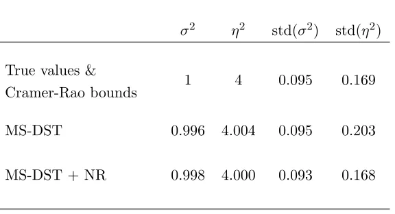
σ2 η2 std(σ2) std(η2)

True values &

Cramer-Rao bounds 1 4 0.095 0.169

MS-DST 0.996 4.004 0.095 0.203

MS-DST + NR 0.998 4.000 0.093 0.168

Table 1: Evaluation of the absolute efficiency of the Multi-Scales DST estimator and the Multi-Scales DST estimator + Newton-Raphson algorithm (MS-DST + NR) with true volatility of 1, noise to signal ratio η

σ = 2, 2048 observations

per day and 5,000 simulations.

but also in finite sample) and consistent estimator of the tick-by-tick volatilityσ2, while the slope is an estimate ofη2_{. Once appropriately rescaled by the number of ticks per day, the resultingIV estimator}

will be called the Multi-Scales DST estimator.

The contemporaneous presence of DST filtering, subsampling and mulstiscale regression makes the analytical computation of asymptotic results very difficult. However, from simulations (Table 1) it turns out that the Multi-Scales DST estimator forσ2 possesses a finite sample variance very close to the Cramer-Rao bounds which now, thanks to the DST results, can be analytically computed (see Appendix C). Moreover, if desired, this small loss of efficiency could be eliminated by using the Multi-Scales DST estimator as initial value in a ML numerical optimization performed, for example, with Newton-Raphson method (as shown in Table 1). A more realistic simulation set up will be employed in the next section to compare different realized volatility estimators.

3

Monte Carlo Simulations

The DGP used in the simulations is a combination of the Heston (1993) SV model for the dynamics of the true price process and the model proposed by Hasbrouck (1999) for the microstructure effects.

In the Heston model the true log price assumes the following continuous time dynamics

dp∗_{(t) = (µ−v(t)/2)dt+σ(t)dB(t) (12)}

reasonable for stocks, will be held constant throughout the simulations. The continuous time model of the true price is simulated at the usual Euler clock of one second.

To this SV model for the dynamics of the true price, we add the Hasbrouck bid-ask model for the observed price. The Hasbrouck model views the discrete bid and ask quotes as arising from the efficient price plus the quote-exposure costs (information and processing costs). Then the bid price is the efficient price less the bid cost rounded down to the next tick and the ask quote is the efficient price plus the ask cost rounded up to the next tick. As in Alizadeh et al. (2002) the model is simplified by assuming that the bid cost and the ask cost are both equal to the minimum tick size.

Then, according to the Hasbrouck model the bid and ask prices are respectively

Bn= ∆⌊Pn∗/∆−1⌋ and An= ∆⌈Pn∗/∆ + 1⌉ (14)

where ∆ represents the tick size, ⌊x⌋ is the floor function, ⌈x⌉ the ceiling one and the unobserved efficient price is P∗

n =ep

∗ n.

Hence, the observed price is given by the following bid-ask model

Pn=Bnqn+An(1−qn) (15)

withqn∼Bernoulli (1/2). Therefore, the observed logarithmic return can be written as

rn= ln

Pn

Pn−1

= ln ⌈Pn/∆ + 1⌉

⌈Pn−1/∆ + 1⌉

+qnln

⌊Pn/∆−1⌋

⌈Pn/∆ + 1⌉

−qn−1ln

⌊Pn−1/∆−1⌋ ⌈Pn−1/∆ + 1⌉

(16)

which would be an MA(1) process in case the true price followed a Brownian motion. Notice that, by adopting the Heston model for the dynamics of the true price, the observed prices do not follow an MA(1) process anymore, making the DST approach formally misspecified. We choose this misspec-ified simulation setting expressly to show the robustness of the DST approach against more general heteroskedastic process in tick time as discussed in section 2.

We first follow Hasbrouck and Alizadeh et al. and choose parameter values which imply a high level of the noise to signal ratio: ∆ = 1/16 and P0 = 45. These values, together with the average

annualized volatility of 20% given by the Heston model for the true price, induce an average noise to signal ratio of about 3.513. Such high level of noise manifests itself as a strong price fluctuation between bid and ask quotes, which generates a highly negative first order-autocorrelationρ(1)≈ −48% for the tick-by-tick returnsrn.

This noise to signal ratio reflects a microstructure impact on the return process which is remarkably large and rarely observed on real data. However, such an extreme setting provides a useful stress test for realized volatility measures and hardens the competition versus daily range-based estimators which are favored under these circumstances.

13_{Following (Oomen 2006) we define the noise to signal ratio as the standard deviation of the noise divided by the}

−300 −20 −10 0 10 20 30 40 0.02

0.04 0.06 0.08 0.1 0.12 0.14 0.16

η/σ = 3.5, observation frequency = 1 min

Fitted DST Min DST MF OLS MF(5) MF(10) EMA Filter Range 5 min avg 5 min sparse

−10 −5 0 5 10 15 0

0.05 0.1 0.15 0.2 0.25 0.3 0.35 0.4 0.45 0.5

η/σ = 3.5, observation frequency = 5 sec

Fitted DST Min DST MF OLS MF(5) MF(10) EMA Filter Range 5 min avg 5 min sparse

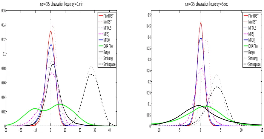
Figure 1: Comparison of the pdf of the estimation errors on the annualized percentage volatility (on average 20%) obtained with an average observation frequency of 1 minute (left panel) and 5 seconds (right panel) and a noise to signal ratio η

σ = 3.5.

We simulate one-day sample paths of 6.5 hours (the typical opening time for stock markets) for 25,000 days. The simulation is repeated for two different values of the total number of price observations per day: M = 390 which corresponds to an average intertrade duration of one minute, and M = 4,680 which corresponds to an average tick arrival time of 5 seconds.

The competing estimators are:

• the two DST estimators: the Minimal DST (Min-DST) is computed with a window length of 30 ticks, while, for the Multi-Scales DST (MS-DST), we construct a series of minimal DST estimator using a sequence ofMj ranging from 2 to 20 ticks and then fit equation (11) through

simple OLS.

• three “simple” Multi-Scales estimators: two Two-Scales estimators with frequency ratio α of 5 and 10, denoted respectively TS(5) and TS(10), and the Multi-Scales Least Square (MS-LS) estimator.14

• the local EMA filter (i.e. calibrated on a single day), which then simply corresponds to a daily MA(1) filter;

14_{About the values chosen for the frequency ratio α, Bandi and Russel (2009) show that for realistic sample sizes}

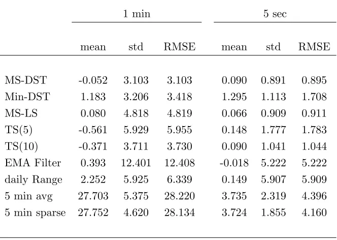
VOLATILITIES ESTIMATES WITH _ση =3.5

1 min 5 sec

mean std RMSE mean std RMSE

MS-DST -0.052 3.103 3.103 0.090 0.891 0.895 Min-DST 1.183 3.206 3.418 1.295 1.113 1.708 MS-LS 0.080 4.818 4.819 0.066 0.909 0.911 TS(5) -0.561 5.929 5.955 0.148 1.777 1.783 TS(10) -0.371 3.711 3.730 0.090 1.041 1.044 EMA Filter 0.393 12.401 12.408 -0.018 5.222 5.222 daily Range 2.252 5.925 6.339 0.149 5.907 5.909 5 min avg 27.703 5.375 28.220 3.735 2.319 4.396 5 min sparse 27.752 4.620 28.134 3.724 1.855 4.160

Table 2: The table report the mean, standard deviation and RMSE of the estimation errors on the annualized percentage volatility (on average 20%) obtained with an average observation frequency of 1 minute (left panel) and 5 seconds (right panel), and a noise to signal ratio η

σ = 3.5.

• two standard realized volatility measures both computed with 5 minute returns but one sampled with an overlapping scheme and then averaged;

• the daily range, as proposed by Parkinson (1980) and recently advocated by Alizadeh et al. (2002) in the context of SV models estimation15 _.

We first consider the case of having 390 observations per day (corresponding to an average one minute frequency) and a noise to signal ratio of 3.5. Table 2 reports the mean, standard deviation and Root Mean Square Error (RMSE) of the estimation errors on the annualized volatility (express as a percentage). Figure 1 shows the probability density functions of those volatility estimation errors.

Given the high level of noise and the relatively small number of observations per day, the estimation of the first order autocorrelation required to calibrate the EMA filter, is very noisy and does not always satisfy the theoretical bound for MA(1) process | ρ(1) |< 1/2 (in the 30% of the cases), leading to a complex MA(1) coefficient θ. In such cases, the EMA filter would fail and we are then forced to impose an artificial floor to ρ(1). But, besides its arbitrariness, this procedure induces unreasonably low volatility estimates (responsible for the left bump presents in the EMA estimator pdf on the left panel of Figure 1). Moreover, under these conditions, the variance of the estimator is extremely large.

15_{Comparison with the recently proposed high frequency range, the so called ”Realized Range-based Variance”}

For the 5 minute realized volatility, the fact that the aggregation from 1 to 5 minute returns is not able to eliminate all the negative autocorrelation, makes this estimator strongly upward biased. In the case of the Minimal DST estimator instead, the aggregation works much better but, due to a relatively low window length of 30 ticks, a small upward bias is still present. Even the daily range suffers from a significant bias but it also has a much larger variance (both, the bias and the variance, are about two times those of the Minimal DST one). Among the three simple Multi-Scales estimators the TS(5) and TS(10) have small negative biases while the MS-LS is virtually unbiased. However, the variance and the RMSE of the TS(10) are lower than the other two simple multi-frequency estimators. Under this extreme setting, the only measure which is still able to remain unbiased and sufficiently precise is the MS-DST estimator, which has, in fact, the lowest RMSE. Moreover, comparing the realized volatility estimators with the one based on the daily range shows that, even in the most unfavorable setting for the realized volatilities, they remain much more accurate than the daily range: the best realized volatility estimator, the MS-DST, possesses, in fact, a RMSE 48% smaller than that of the daily range.

Keeping the same level of noise, we repeat the simulation at 5 second frequency (which means 4,680 observations per day). With twelve times more data the realized volatility measures are much more precise: the local EMA filter has less failings (5%) and lower variance, while the 5 minute realized volatilities (thanks to the longer aggregation period) have smaller, but still significant, biases. Although smaller than the biases of the 5 minute realized volatilities, the Minimal DST still shows a bias with this high level of noise. The Zhang et al. estimators become both unbiased with the TS(10) having a smaller variance than the TS(5). The MS-DST and the MS-LS estimators are both unbiased and equally very accurate, remaining the best choices among the estimators considered.

In practice, however, financial time series present a noise to signal ratio at tick-by-tick level that usually lies between 0.5 and 2. But, even with such a moderate level of noise, a naive high frequency realized volatility measure would be from one to three times the actual one. We then repeat the simulation with a more realistic noise to signal ratio of 1.5 for both observation frequencies. Table 3 and Figure 2 summarize the results.

At the 1 minute frequency the daily range and the local EMA filter are unbiased but quite inac-curate while the realized volatilities based on 5–minute have again a large bias. The MS-DST and the other Multi-Scales estimators are the most accurate with the MS-LS having a slightly smaller bias and variance than the others.

At the 5 second frequency, with a moderate level of noise and a large number of data, the EMA filter starts to have a much lower variance and the 5 minute measures much lower biases. Nevertheless, they can still not compete with the MS-DST and the three other Multi-Scales estimators which become extremely precise and accurate under this setting.

−150 −10 −5 0 5 10 15 20 0.02 0.04 0.06 0.08 0.1 0.12 0.14 0.16 0.18 0.2

η/σ = 1.5, observation frequency = 1 min

Fitted DST Min DST MF OLS MF(5) MF(10) EMA Filter Range 5 min avg 5 min sparse

−100 −8 −6 −4 −2 0 2 4 6 8 10 0.1 0.2 0.3 0.4 0.5 0.6 0.7

η/σ = 1.5, observation frequency = 5 sec

Fitted DST Min DST MF OLS MF(5) MF(10) EMA Filter Range 5 min avg 5 min sparse

Figure 2: Comparison of the pdf of the estimation errors on the annualized percentage volatility (on average 20%) obtained with an average observation frequency of 1 minute (left panel) and 5 seconds (right panel) and a noise to signal ratio η

σ = 1.5.

−150 −10 −5 0 5 10 15 20 0.05

0.1 0.15 0.2

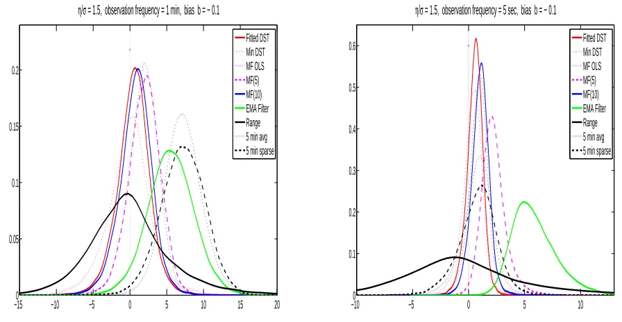
η/σ = 1.5, observation frequency = 1 min, bias b = − 0.1

Fitted DST Min DST MF OLS MF(5) MF(10) EMA Filter Range 5 min avg 5 min sparse

−100 −5 0 5 10 0.1 0.2 0.3 0.4 0.5 0.6

η/σ = 1.5, observation frequency = 5 sec, bias b = − 0.1

Fitted DST Min DST MF OLS MF(5) MF(10) EMA Filter Range 5 min avg 5 min sparse

Figure 3: Comparison of the pdf of the estimation errors on the annualized percentage volatility (on average 20%) obtained with an average observation frequency of 1 minute (left panel) and 5 seconds (right panel), a noise to signal ratio η

VOLATILITIES ESTIMATES WITH _ση = 1.5

Unbiased Bernoulli

1 min 5 sec

mean std RMSE mean std RMSE

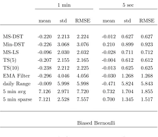
MS-DST -0.220 2.213 2.224 -0.012 0.627 0.627 Min-DST -0.226 3.068 3.076 0.210 0.899 0.923 MS-LS -0.096 2.030 2.032 -0.028 0.711 0.712 TS(5) -0.207 2.155 2.165 -0.004 0.612 0.612 TS(10) -0.238 2.212 2.225 -0.013 0.625 0.625 EMA Filter -0.296 4.046 4.056 -0.030 1.268 1.268 daily Range -0.009 5.998 5.998 -0.471 5.824 5.843 5 min avg 7.126 2.971 7.720 0.732 1.704 1.855 5 min sparse 7.121 2.528 7.557 0.700 1.345 1.517

Biased Bernoulli

1 min 5 sec

MS-DST 0.389 2.234 2.267 0.675 0.717 0.984 Min-DST -0.153 3.077 3.081 0.329 0.904 0.963 MS-LS 1.722 2.070 2.693 0.831 0.817 1.166 TS(5) 1.888 2.150 2.862 2.200 1.081 2.451 TS(10) 0.726 2.214 2.330 1.023 0.791 1.294 EMA Filter 5.467 3.136 6.303 5.840 1.979 6.167 daily Range -0.128 5.823 5.825 -0.457 5.926 5.944 5 min avg 7.103 2.978 7.702 0.754 1.741 1.898 5 min sparse 7.105 2.549 7.548 0.719 1.370 1.548

Table 3: The table reports the mean, standard deviation and RMSE of the estimation errors on the annualized percentage volatility (on average 20%) obtained with an average observation frequency of 1 minute (left panel) and 5 seconds (right panel), a noise to signal ratio η

σ = 1.5 and, for the bottom panel, a biased Bernoulli process with

by introducing a correlation in the sequence at which bid and ask prices arrive16. Hence, instead of having an “unbiased” Bernoulli(1/2) for the qn process, we construct a Bernoulli process which

produces autocorrelation inqn. This “biased” Bernoulli is obtained by takingqn= Bernoulli (1/2 +b)

if qn−1 = 1 and qn = Bernoulli (1/2−b) if qn−1 = 0. We choose b =−0.10 which induces a second

order autocorrelation of about−6%.

Now, in the presence of not i.i.d. microstructure noise, the local EMA filter, which was unbiased, becomes highly biased at both frequencies (see Figure 3). Also the TS and MS-LS estimators are now showing a positive bias. Among all the realized volatility estimators the DST measures are the ones with the smallest bias and smallest RMSE, showing a high degree of robustness against more general microstructure noise contaminations (as analytically described in the previous section).

Summarizing the results of the simulation study, we can draw the following conclusions. The daily range estimator is always inferior to the realized volatility ones. The realized volatilities with 5 minute returns are often significantly biased and inaccurate. The local EMA filter gives satisfactory results only in the presence of a high number of observations and a low level of i.i.d. noise. Although more precise in general, similar considerations can be made for the simple MS estimators (TS and MS-LS). When the microstructure noise is moderate and i.i.d. the simple MS estimators are almost as accurate as the MS-DST and hence close to the optimal Cramer-Rao efficiency bound (since, as shown in section 2.4, the MS-DST is very close to the full efficiency of the Cramer-Rao bounds). In particular, the MS-LS seems to be particularly efficient in exploiting the information contained in the data when a relatively small number of observations is available (perhaps due to its ability to extract information from many frequencies), while the TS(5) and TS(10) are at their best when the number of observations increases. However, when the microstructure noise increases and deviations from the i.i.d. structure arise, the discrepancy between the simple MS estimators and the MS-DST starts to increase due to a higher level of robustness of the DST approach. Therefore, the overall winner that seems to arise from this volatility estimation “horse race” is the MS-DST which shows the highest level of precision and robustness across a wide range of microstructure noise contaminations.

4

Empirical application

To verify the behavior of volatility estimators when the microstructure noise is not an i.i.d. process, we analyze six years of tick-by-tick data (from January 1998 to October 2003) for the following three future contracts: the S&P 500 stock index future, the 30 years U.S. Treasury Bond future and the Italian stock index future FIB 30. In a base asset mapping approach (as the one of RiskMetrics), those three major future contracts can be seen as the reference liquid base assets for, respectively, the US stock and bond market and the Italian stock market.

In order to analyze the dependence structure of the microstructure noise in those series, we

in-16 _{Hasbrouck and Ho (1987) suggest that positive autocorrelation at lag lengths greater than one may be the result}

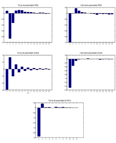
vestigate the behaviour of the autocorrelation of tick-by-tick returns. This tick-time autocorrelation analysis shows significant departure from the standard i.i.d. assumption for the microstructure noise. In fact, more complex structures than that of a simple MA(1) expected under the standard i.i.d. assumption, were found in all the three series. These patterns are independent of the inclusion or censoring of all zero trade-by-trade returns which, in all the three assets, usually represent only a small percentage of the total number of trade-by-trade returns.

Such autocorrelation patterns of the tick-by-tick returns are instead consistent with more complex ARMA structure for the microstructure noise. In fact, simulating the Hasbrouck model with those ARMA structures for the noise, leads to exactly the same autocorrelation functions observed in the data. In particular, those patterns are consistent with a microstructure noise having an MA(1) struc-ture for the FIB, an MA(2) (at least) for the S&P and a strong oscillatory AR(1) for the US bond17 (see Figure 4).

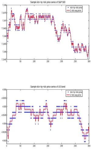
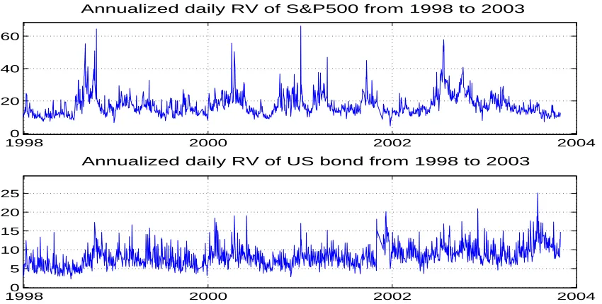
To overcome the problem of a complex ARMA structure in the autocorrelation of tick-by-tick returns of the S&P and US bond, we first notice that, in both cases, a simple aggregation of two ticks returns almost restore the MA(1) autocorrelation pattern typical of the i.i.d. assumption for the microstructure noise (see Figure 5). Therefore, applying the MS-DST estimator to the two-ticks returns of the S&P and US bond series, we can still obtain a highly precise evaluation of the realized volatilities of the two assets and closely follow their time series dynamics (see Figure 6).

Obviously, in empirical analysis the true volatility is not observable, hence no direct evaluation criteria of the quality of the volatility estimators exist. However, general indirect criteria can be employed.

First of all, the unconditional mean of daily volatilities obtained with high frequency estimators should not be significantly different from the unconditional mean volatility obtained with lower fre-quency returns. We asses this property for the MS-DST estimator by computing its volatility signature plot. Figure 7 shows the volatility signature plot of the standard and MS-DST realized volatility mea-sures for the three assets, averaged over the whole six years period. Ideally, for estimators which are robust against microstructure effects the scaling should appear as a flat line in the volatility signa-ture plot. The top panel of Figure 7 refers to the scaling of S&P 500 fusigna-ture showing a moderate but clear impact of the market microstructure on the standard realized volatility measure and the presence of a mild lower frequency autocorrelation. The MS-DST estimator correctly discounts mar-ket microstructure effects on volatility while it retains the residual lower frequency autocorrelation which is responsible for its scaling behavior to be not completely flat. The middle and bottom panels are respectively the FIB 30 and U.S. Bond future. In both cases market microstructure noise has a strong impact on the standard measure of realized volatility inducing larger biases as the frequency increases while the MS-DST estimator, remaining reasonably flat at any frequency, confirms its ability to properly filter out market microstructure effects.

Under the hypothesis of an underlying continuous time diffusion process for the logarithm price,

17 _{The analysis of the market microstructure determinants and specific institutional constraints that would lead to}

0 50 100 150 200 250 300 7.2445

7.245 7.2455 7.246 7.2465 7.247 7.2475 7.248

Sample tick−by−tick price series of S&P 500

tick−by−tick price 2−tick avg price

0 50 100 150 200 250 300

4.503 4.5035 4.504 4.5045 4.505 4.5055 4.506

Sample tick−by−tick price series of US bond

tick−by−tick price 2−tick avg price

1 2 3 4 5 6 7 8 9 10 11 12 13 14 15 −0.1

−0.08 −0.06 −0.04 −0.02 0 0.02

Tick−by−tick autocorrelation SP500

1 2 3 4 5 6 7 8 9 10 11 12 13 14 15

−0.1 −0.08 −0.06 −0.04 −0.02 0 0.02

2 ticks returns autocorrelation SP500

1 2 3 4 5 6 7 8 9 10 11 12 13 14 15

−0.6 −0.4 −0.2 0 0.2 0.4

Tick−by−tick autocorrelation US Bond

k−values

1 2 3 4 5 6 7 8 9 10 11 12 13 14 15

−0.16 −0.14 −0.12 −0.1 −0.08 −0.06 −0.04 −0.02 0 0.02

2 ticks returns autocorrelation US bond

1 2 3 4 5 6 7 8 9 10 11 12

−0.3 −0.25 −0.2 −0.15 −0.1 −0.05 0 0.05

Tick−by−tick autocorrelation for FIB 30

19980 2000 2002 2004 20

40 60

Annualized daily RV of S&P500 from 1998 to 2003

19980 2000 2002 2004

5 10 15 20 25

Annualized daily RV of US bond from 1998 to 2003

Figure 6: Time series of the annualized realized volatility computed with the MS-DST estimator on the two ticks returns for the S&P 500 (top panel) and US Bond (bottom panel) futures from 1998 to 2003.

another indirect criterion can be considered to asses the quality of realized volatility measures in em-pirical applications. In fact, if the log-price follows a SV diffusion the model for daily returns could be written as rt = σtzt where zt ∼ i.i.d. N(0,1). Hence, the 1-day return would be conditionally

Gaussian with variance equal to the integrated variance. The normality of zt is justified by

appeal-ing to the Central Limit Theorem for mixappeal-ing process aggregated over a reasonable length of time (such as daily for highly traded assets). Therefore, if a volatility measure adequately estimates the integrated volatility, the corresponding standardized returns should be normally distributed. We test this condition using the Jarque-Bera normality test on returns standardized by the 30 minute realized volatility18_{, MS-DST realized volatility and the daily range}19_.

Table 4 reports the results. In all three cases, daily raw returns are highly leptocurktic as expected, while returns standardized by daily ranges become highly thin tailed and remain far from normal. Returns standardized by 30 minute realized volatilities become excessively thin tailed for the S&P and US Bond while remaining too fat tailed for the FIB 30 and clearly failing the Jarque-Bera tests

18_{This choice of a somewhat lower frequency of 30–minute instead of an higher one, is motivated by the need of having}

an unbiased estimator of the daily volatility. Higher frequency realized volatility measures (such as with 1–minute or 5–minute returns) would in fact suffers, on this data set, of a large positive bias that by itself would heavily distort the criterion here considered.

19_{The EMA filter estimator has not been included here because, as shown in the simulations, it is sensitive to the}

100 101 102 103 15

16 17 18 19 20 21 22 23 24

Signature plot of S&Pdaily RV from 1998 to 2003

∆ t in n° of ticks: from 1 tick = 8sec to 1000 ticks = 134min

RV

Fitted DST Standard RV

100 101 102 103

18 20 22 24 26 28 30 32 34

Signature plot of FIB30 daily RV from 1998 to 2003

∆ t in n° of ticks: from 1 tick = 9sec to 1000 ticks = 154min

RV

Fitted DST Standard RV

100 101 102 103

6 8 10 12 14 16 18 20

Signature plot of US Bond daily RV from 1998 to 2003

∆ t in n° of ticks: from 1 tick = 18sec to 1000 ticks = 292min

RV

MS−DST Standard RV

in all the three cases. Whereas for the MS-DST standardized returns, Jarque-Bera test cannot be rejected for both the stock index future S&P and FIB. However, for the US Bond future, even though among the three competing estimators the MS-DST standardized returns remain by far the closest to the standard normal, the Jarque-Bera test is rejected. The rejection is due to a value of the kurtosis excessively smaller than three, meaning that the MS-DST measure tends to overestimate the “true” integrated volatility of the Bond future process. However, since the realized volatility consistently estimates the quadratic variation (which includes the contributions of jumps) and not the integrated volatility (which only considers the contribution of the continuous part), such overestimation could be due to the presence of a large jump components in the Bond future series. Indeed, the fact that the relative contribution of jumps is higher in bond series compared to stock indices, has been recently found by Andersen Bollerslev and Diebold (2007) and is consistent with the empirical evidence of the fixed income market being the most responsive to macroeconomic news announcements (Andersen, Bollerslev, Diebold and Vega 2003).

In summary, the analysis conducted on the empirical data confirms the ability of the MS-DST estimators to accurately and reliably estimate daily realized volatility, thus confirming the results obtained in the Monte Carlo simulation analysis.

5

Conclusions

The presence of microstructure effects represent a challenging problem for realized volatility measures making the naive realized volatility computed at short time intervals highly biased. In this study new realized volatility measures based on Multi-Scale regression and Discrete Sine Transform (DST) approaches are presented. We show that Multi-Scales estimators similar to that recently proposed by Zhang (2006) can be constructed within a simple regression based approach by exploiting the linear relation existing between the market microstructure bias and the realized volatilities computed at different frequencies. These regression based estimators can be further improved and robustified by using the DST approach to filter market microstructure noise. This approach is justified by the theoretical result regarding the ability of the DST to diagonalize exactly an MA(1) process and approximately an MA(q) one. Hence, we utilize the DST orthonormal basis decomposition to optimally disentangle the underlying efficient price signal from the time-varying nuisance component contained in tick-by-tick return series. The robustness of the DST approach with respect to more general dependent structures of the microstructure noise is also analytically shown.

Std. Dev Kurtosis Skewness Jarque-Bera Probability

S&P 500

Raw returns 19.395 6.540 -0.010 734.828 0.000

MS-DST-std. returns 1.024 2.764 0.019 3.344 0.187

30 min-std. returns 1.066 2.432 -0.026 19.044 0.000

Range-std. returns 0.922 1.754 -0.037 91.316 0.000

FIB 30

Raw returns 24.4786 6.853 -0.236 829.114 0.000

MS-DST-std. returns 1.106 2.890 0.146 5.370 0.068

30 min-std. returns 1.577 4.171 -0.036 75.720 0.000

Range-std. returns 0.912 1.752 0.049 86.137 0.000

US Bond

Raw returns 8.6578 4.101 -0.423 113.056 0.000

MS-DST-std. returns 0.966 2.517 -0.110 16.464 0.000

30 min-std. returns 1.000 2.283 -0.094 32.211 0.000

Range-std. returns 0.887 1.766 -0.094 91.326 0.000

Table 4: Comparison of sample distribution properties of daily raw and standardized returns of FIB 30, S&P 500 and thirty years Bond futures from 1998 to 2003. Standardized returns are computed using MS-DST, 30 minute realized volatility and daily range.

Monte Carlo simulations based on a realistic model for microstructure effects and volatility dynam-ics, show the superiority of MS-DST estimators compared to alternative local volatility proxies such as the TS and MS-LS estimators, the daily range, the EMA filter and 5 minute realized volatilities. The MS-DST estimator results to be the most accurate and robust across a wide range of noise to signal ratios and types of microstructure noise contaminations. The empirical analysis based on six years of tick-by-tick data for S&P 500 index-future, FIB 30, and 30 years U.S. Tresaury Bond future, seems to confirm Monte Carlo results.

Appendix A: Dependent Noise

In the presence of MA(q−1) dependent noise, the observed returns in tick time become an MA(q) process which can be written as

rn=σ˜ǫn+ q

X

i=1 ηi

ω(ni)−ω

(i)

n−i

with ˜ǫn∼IID (0,1) andω(ni)∼IID (0,1). In this more general case the variance of the Minimal DST component becomes

σ2M =E

c(minM)(n)c

(M)

min(n)

=σ2+

q

X

i=1

ηi2F(M, i)

where

F(M, i) = 2

M+ 1

M+ 1−(M+ 1−i) cos πi

M+ 1−cot

π M+ 1sin

πi M+ 1

.

BecauseF(M, i) can be approximated as

F(M, i) =π2 i 2

M2 −2π 2 i3

M3

1 +3

i− 1 i2 +O i4 M4

whenM/q→ ∞, we obtain that

σ2M ≃σ2+

π2 M2

q

X

i=1

(i ηi)2

Appendix B: Multi-Scales Regression with Endogenous Noise

Writing the observed tick-by-tick return asrn=r∗n+unwithrn∗=p∗n−p∗n−1the efficient return andunthe endogenous

noise, we model the correlation between the microstructure noise and the dynamics of the efficient price by assuming the following form forun(as in Hansen and Lunde 2006):

un=ρ(p∗n−p ∗

n−1) +η(ωn−ωn−1) =ρrn∗+η(ωn−ωn−1). (B-1)

We then have thatE[un] = 0,E[ut2] =ρ2σ2n+ 2η2 andE[rn∗un] =ρσ2n, whileE[r∗n−sun] = 0 fors >0.

Therefore, the conditional expectation of the daily realized variance RV(kj) _{computed with observed returns of}

different tick-lengthskj is

EhRV(kj)i_{=IV +N}(kj)_(ρ2_σ2_{+ 2η}2_{) + 2N}(kj)_ρσ2_{=IV +N}(kj)_{(ρ(2 +ρ)σ}2_{+ 2η}2_{) (B-2)}

whereN(kj)_{is the number ofk}

j-returns in the day andσ2=IV /N the average variance per tick. The terms proportional

toN(kj) _{stem from the facts that the endogenous noise arise only when an observation is made (thus the termN}(kj)₎

and the correlation betweenkjtick return (r∗(kj)) and microstructure noise remains the same irrespective of their tick

lengths since

E[r∗(kj)

n un] =E[(r∗n−kj +r ∗

n−kj+1+...+r ∗

n−1+r∗n)un] =E[r∗nun] =ρσn2. (B-3)

Appendix C: Exact MA(1) Likelihood, Cramer-Rao bounds and

ab-solute efficiency

Thanks to the universality of the eigenvectors, we can obtain a diagonalization of the variance-covariance matrix of MA(1) processes which does not depend on the parameters to be estimated. Collecting the M eigenvectors of Ω in the MxM characteristic matrix Ψ = [ϕ1ϕ2..., ϕM], we can project the return vector onto the orthogonal space of the

principal componentC= Ψ⊤_{R,which is aMx1 vector distributed asC∼N(0,Λ), where Λ is theMxM diagonal matrix}

containing theM eigenvalues of the tridiagonal matrix Ω20_{. Therefore, the likelihood function ofRcan be rewritten in}

terms of the principal components vectorC as

f(C) = q 1 (2π)Mdet Λ

exp

−1

2C ⊺_Λ−1_C

= q 1

(2π)MQM n=1λn

exp " −1 2 M X n=1 c2 n λn #

20_{In fact,E[CC}⊤_{] =}

E[Ψ⊤_RR⊤_{Ψ] = Ψ}⊤

and

lnfθ(C) = −

M

2 ln 2π− 1 2

M

X

n=1

lnλn−

1 2 M X n=1 c2 n λn

Then, from the linear equation (5) we readily obtain

∂λn

∂θ =

1 4 sin2 πn

2(M+1) !

and ∂

2_λ

n

∂θi∂θk

= 0 for i, k= 1,2

and hence, we are now able to analytically derive the equations for the Score and the Hessian

∂lnfθ(C)

∂θi = 1 2 M X n=1 c2 n λ2 n − 1 λn ∂λn ∂θi ; ∂

2_lnf

θ(C)

∂θi∂θk

=− M X n=1 c2 n λ3 n − 1

2λ2

n ∂λn ∂θi ∂λn ∂θk

Therefore, thanks to equation (5) and (6) we are able to explicitly compute the Fisher Information matrix of an MA(1) process, which reads

Iik=−E

∂2_lnf

θ(C)

∂θi∂θk

=1 2 M X n=1 1 λ2 n ∂λn ∂θi ∂λn ∂θk

With each element of the matrix given by

I11=

1 2 M X n=1 1 λ2 n

, I22= 8

M X n=1 1 λ2 n sin4 _πn

2 (M+ 1)

, I12=I21= 2

M X n=1 1 λ2 n sin2 _πn

2 (M+ 1)

Then the Cramer-Rao bounds of ˆσ2 and ˆη2 can now be given in closed form as

var ˆσ2> I22

I11I22− I122

and var ˆη2> I11

I11I22− I122

These results have two important implications. First they obviously permit to evaluate the absolute efficiency of volatility

estimators. Second numerical optimization of the exact likelihood is greatly simplified. In fact, given that the principal

components do not depend on the parameter, the orthogonalization of the returns process needs to be done only once

rather then at each iteration as it occurs using Cholesky factorization (see Hamilton 1994).

References

A¨ıt-Sahalia, Y., Mykland, P. A. and Zhang, L.: 2005, How often to sample a continuous-time process in the

presence of market microstructure noise,Review of Financial Studies18_{, 351–416.}

A¨ıt-Sahalia, Y., Mykland, P. A. and Zhang, L.: 2006, Ultra high frequency volatility estimation with dependent

microstructure noise, Manuscript. Princeton University, University of Chicago and University of Illinois.

An´e, T. and Geman, H.: 2000, Order flow, transaction clock, and normality of asset returns,Journal of Finance

55_{(5), 2259–84.}

Alizadeh, S., Brandt, M. W. and Diebold, F. X.: 2002, Range-based estimation of stochastic volatility models,

Journal of Finance 57_{(3), 1047–90.}

Andersen, T. G., Bollerslev, T. and Diebold, F. X.: 2005, Parametric and nonparametric volatility measurement,

inY. A¨ıt-Sahalia and L. P. Hansen (eds),Handbook of Financial Econometrics, North Holland, Amsterdam.

Andersen, T. G., Bollerslev, T. and Diebold, F. X.: 2007, Roughing it up: Including jump components in

the measurement, modeling, and forecasting of return volatility, The Review of Economic and Statistics

Andersen, T. G., Bollerslev, T., Diebold, F. X. and Labys, P.: 2001a, The distribution of exchange rate volatility,

Journal of the American Statistical Association96_{, 42–55.}

Andersen, T. G., Bollerslev, T., Diebold, F. X. and Labys, P.: 2001b, Great realizations,Risk13_{, 105–108.}

Andersen, T. G., Bollerslev, T., Diebold, F. X. and Vega, C.: 2003, Micro effects of macro announcements:

Real-time price discovery in foreign exchange,American Economic Review93_{, 38–62.}

Bandi, F. and Russell, J. R.: 2005, Microstructure noise, realized volatility, and optimal sampling. Working Paper, Graduate School of Business, University of Chicago.

Bandi, F. and Russell, J. R.: 2009, Market microstructure noise, integrated variance estimators, and the accuracy

of asymptotic approximations,Journal of Econometrics, forthcoming.

Barndorff-Nielsen, O. E., Hansen, P. R., Lunde, A. and Shephard, N.: 2004, Regular and modified

kernel-based estimators of integrated variance: The case with independent noise. Working paper,

http://ssrn.com/abstract=620203.

Barndorff-Nielsen, O. E., Hansen, P. R., Lunde, A. and Shephard, N.: 2008, Designing realised kernels to

measure the ex-post variation of equity prices in the presence of noise,Econometrica. Forthcoming.

Barndorff-Nielsen, O. E. and Shephard, N.: 2001, Non-gaussian ornstein-uhlembech-based models and some of

their uses in financial economics, Journal of the Royal Statistical SocietySeries B_{(63), 167–241.}

Barndorff-Nielsen, O. E. and Shephard, N.: 2002a, Econometric analysis of realized volatility and its use in

estimating stochastic volatility models,Journal of the Royal Statistical SocietySeries B_{(64), 253–280.}

Barndorff-Nielsen, O. E. and Shephard, N.: 2002b, Estimating quadratic variation using realized variance,

Journal of Applied Econometrics 17_{(5), 457–477.}

Barndorff-Nielsen, O. E. and Shephard, N.: 2005, How accurate is the asymptotic approximation to the

distri-bution of realized volatility?,inD. W. F. Andrews and J. H. Stock (eds),Identification and Inference for

Econometric Models. A Festschrift in Honour of T.J. Rothenberg, Cambridge University Press, pp. 306–331.

Blume, M. and Stambaugh, S.: 1983, Biases in computed returns,Journal of Financial Economics12_{, 387–404.}

Bollen, B. and Inder, B.: 2002, Estimating daily volatility in financial markets utilizing intraday data,Journal

of Empirical Finance186_.

Christensen, K. and Podolskij, M.: 2006, Realized range-based estimation of integrated variance, Journal of

Econometrics. To appear in.

Clark, P. K.: 1973, A subordinated stochastic process model with finite variance for speculative prices,

Econo-metrica41_{(1), 135–55.}

Cohen, K., S., M., R., S. and D., W.: 1981, Transaction costs, order placement strategy, and existence of the

bid-ask spread,Journal of Political Economy89_{, 287–305.}

Comte, F. and Renault, E.: 2001, Long memory in continuous time stochastic volatility models,Mathematical

Finance8_{, 291–323.}

Corsi, F., Zumbach, G., M¨uller, U. A. and Dacorogna, M.: 2001, Consistent high-precision volatility from

high-frequency data,Economic Notes30_{(2), 183–204.}

Elliott, J., F.: 1953, The characteristic roots of certain real symmetric matrices,Technical report, University of

French, K. R. and Roll, R.: 1986, Stock return variances : The arrival of information and the reaction of traders,

Journal of Financial Economics 17_{(1), 5–26.}

Glosten, L.: 1994, Is the electronic open limit-order book inevitable?,Journal of Finance 49_{, 1127–1161.}

Glottlieb, G. and Kalay, A.: 1985, Implication of the discreteness of observed stock prices,Journal of Finance

40_{, 135–153.}

Gregory, Robert, T. and Karney, D.: 1969, A collection of matrices for testing computational algorithms,

Wiley-Interscience.

Hamilton, J.: 1994,Time Series Analysis, Princeton: Princeton University Press.

Hansen, P. R. and Lunde, A.: 2004, An unbiased measure of realized variance. Working Paper, Department of Economics, Stanford University.

Hansen, P. R. and Lunde, A.: 2006, Realized variance and market microstructure noise, Journal of Business

and Economic Statistics24_(127-218).

Harris, L.: 1990, Estimation of stock price variances and serial covariances from discrete observations,Journal

of Financial and Quantitative Analysis25_{(3), 291–306.}

Hasbrouck, J.: 1993, Assessing the quality of a security market: a new approach to transaction-cost

measure-ment,Review of Financial Studies6_{(1), 191–212.}

Hasbrouck, J.: 1996, Modelling market microstructure time series, in G. S. Maddala and C. R. Rao (eds),

Statistical Methods in Fianance, Vol. 14 of Handbook of Statistics, North Holland, Amsterdam, pp. 647– 692.

Hasbrouck, J.: 1999, The dynamichs of discrete bid and ask quotes,Journal of Finance 54_{, 2109–42.}

Hasbrouck, J. and Ho, T.: 1987, Order arrival, quote behavior, and the return-generating process,Journal of

Finance42_{, 1035–48.}

Heston, S.: 1993, A closed-form solution for options with stochastic volatility with applications to bonds and

currency options,Review of Financial Studies6_{, 327–343.}

Lan, Z.: 2006, Efficient estimation of stochastic volatility using noisy observations: A multi-scale approach.,

Bernoulli12_{, 1019–1043.}

Martens, M. and van Dijk, D.: 2007, Measuring volatility with the realized range, Journal of Econometrics

138_{(1), 181–207.}

Merton, R. C.: 1980, On estimating the expected return on the market: An exploratory investigation,Journal

of Financial Economics 8_{, 323–61.}

Nolte, I. and Voev, V.: 2008, Estimating high-frequency based (co-) variances: A unified approach. Working Paper.

Oomen, R. C.: 2005, Properties of bias-corrected realized variance under alternative sampling schemes,Journal

of Financial Econometrics 3_{(4), 555–577.}

Oomen, R. C.: 2006, Properties of realized variance under alternative sampling schemes,Journal of Business