Semi-supervised heterogeneous evolutionary co-clustering

(1)

Rochester Institute of Technology

RIT Scholar Works

Theses Thesis/Dissertation Collections

12-1-2012

Semi-supervised heterogeneous evolutionary

co-clustering

Pankaj Andhale

Follow this and additional works at:http://scholarworks.rit.edu/theses

This Thesis is brought to you for free and open access by the Thesis/Dissertation Collections at RIT Scholar Works. It has been accepted for inclusion in Theses by an authorized administrator of RIT Scholar Works. For more information, please [email protected].

Recommended Citation

(2)

Semi-supervised Heterogeneous Evolutionary

Co-clustering

by

Pankaj Andhale

A Master’s Thesis Submitted in Partial Fulfillment of the Requirements for the Degree of Master of Science in Computer Science

Supervised by

Dr. Manjeet Rege

Department of Computer Science

B. Thomas Golisano College of Computing and Information Sciences Rochester Institute of Technology

Rochester, New York December 2012

Approved By:

Dr. Manjeet Rege

Department of Computer Science Primary Adviser

Dr. Reynold Bailey

Department of Computer Science Reader

Prof. Henry Etlinger

(3)

c

Copyright 2012 by Pankaj Andhale

(4)

Abstract

One of the challenges of the machine learning problem is the absence of sufficient

num-ber of labeled instances or training instances. At the same time generating labeled data is

expensive and time consuming. The semi-supervised approach has shown promising

re-sults to solve the problem of insufficient or fewer labeled instance datasets. The key

chal-lenge is incorporating the semi-supervised knowledge into the heterogeneous data which is

evolving in nature. Most of the prior work that uses semi-supervised knowledge has been

performed on heterogeneous static data. The semi-supervised knowledge is incorporated

into data which aid the clustering algorithm to obtain better clusters. The semi-supervised

knowledge is provided as constrained based or distance based. I am proposing a

frame-work to incorporate prior knowledge to perform co-clustering on the evolving

heteroge-neous data. This framework can be used to solve a wide range of problems dealing with

text analysis, web analysis and image grouping. In the semi-supervised approach we

incor-porate the domain knowledge by placing the constraints which aid the clustering process

in performing effective clustering of the data. In the proposed framework, I am using the

constraint based semi-supervised non-negative matrix factorization approach to obtain the

co-clustering on the heterogeneous evolving data. The constraint based semi-supervised

approach uses the user provided must-link or cannot-link constraints on the central data

type before performing co-clustering. To process the original datasets efficiently in terms

of time and space I am using the low rank approximation technique to obtain the sparse

(5)

List of Figures

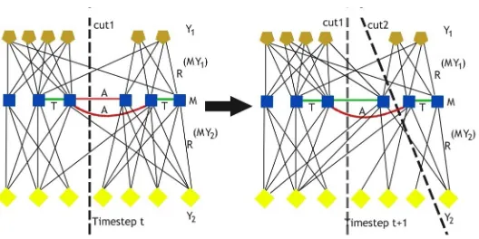
3.1 Semi-supervised co-clustering of heterogeneous star structure relational evolving data at time steptandt+ 1 . . . 11

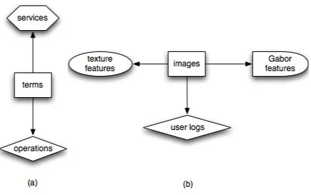
4.1 (a).Web service and (b). Image datasets forming a star structure schema where, (a). The terms forms the central type and is connected to service and operations. (b). The image forms cental type and is connected to texture feature, Gabor feature and user logs . . . 20 4.2 Detecting the number of clusters in the current time step data t using

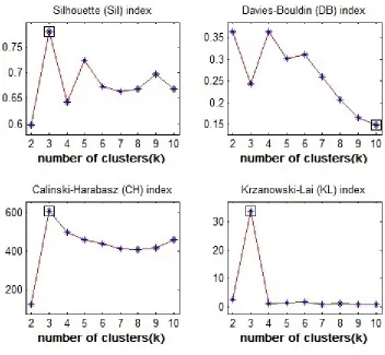
Krzanowski-Lai, Davies-Bouldin index, Silhouettes and Calinski-Harabasz index tech-niques . . . 22 4.3 Semi-supervised co-clustering accuracy is measured by placing 0, 1, 2 and

4 percent constraint on evolving web service dataset from time step t0 to t7 where the numbers of instances features are shifted, added or removed

from clusters. . . 23 4.4 Measuring the semi-supervised co-clustering accuracy by varying the value

ofα while keeping the constraint percentage constant on the web service dataset . . . 24 4.5 Comparing the results of SSHECC when the percentage of evolved

in-stances change keeping the constraints andαconstant on the web service dataset . . . 25 4.6 Visual representation of must-link and cannot-link constraint on the image

and the user log dataset at time step t consisting of 5 row and column clusters. The constraints are placed on the central type data. i.e. images represented by green and red lines . . . 26 4.7 Semi-supervised co-clustering accuracy is measured by placing 0, 1 and

2 percent constraint on the evolving image dataset from time stept0 tot7

(7)

4.8 Measuring the semi-supervised co-clustering accuracy on image dataset where instances are evolved randomly keeping the percentage constraint andαconstant . . . 28 4.9 Semi-supervised co-clustering accuracy is measured by placing 0, 1, 3 and

5 percent constraint on the evolving synthetic dataset from time stept0 to t7 where the numbers of instances features are shifted, added or removed

(8)

List of Tables

(9)

1. Introduction

The sophistication in the data gathering techniques has led to the generation of large amounts

of unstructured data. This data is heterogeneous and evolving in nature, and efficient

tech-niques to process and analyze the data need to be developed. In the absence of background

knowledge or the characteristics of the data and class labels, to gain insightful information

about the given dataset, a clustering technique is implemented. Clustering is a process of

grouping similar instances together[15][16]. Only one dimension of data is used in

cluster-ing.

Co-clustering is a technique which explores the dual dimension of the data, by

identi-fying natural grouping based not only on the instance similarity, but also uses the feature

similarity[9][2] as well as the instance feature relationship is used. The co-clustering

ap-proaches are either graph theory, information theory or probability based models[7]. The

graph theory approach such as Spectral Graph Partition(SVD) [2], Consistent Bipartite

Graph Copartitioning (CBGC)[11] and iso-perimetric co-clustering [27] have been used to

perform co-clustering. Most of the real world data mining problems are heterogeneous in

nature, so a star structure relational heterogeneous data model is used to simulate these

problems [7].

To deal with the heterogeneous data in the evolving environment such as blogs, social

networks, professional networks etc. we have to handle the incoming data at each time

step. The clustering should be based on the current characteristics of the data [5]. At

the same time it should not deviate too much from the previous time step [8]. As in the

real world we do not frequently observe a drastic shift in the associations between the

(10)

and capture the evolving changes in the data at every time step simultaneously and represent

the clusters associated with current time step data and close enough to the previous time

step data. Nathan Green has performed the co-clustering on the evolving data using the

spectral approach[23]. The non-negative matrix factorization approach for co-clustering is

the most efficient way as it requires less space and time for computation and also the results

obtained are intuitive [7]. The heterogeneous data co-clustering is implemented using the

simultaneous clustering of related data types. Our approach will be dealing with the star

structure schema, where the central type is connected to all other types. To simulate a star

structure heterogeneous environment consider the interrelations of words, documents and

categories in the text mining field. The text corpus document is the central type which is

connected to the words and categories. Single sided constraints are placed on the central

type i.e. documents. Using the distance learning metric [7] the distances within the similar

data points will be reduced and the semi-supervised knowledge is incorporated. Finally

co-clustering is performed using the non-negative matrix factorization.

Semi-supervised is a learning approach which combines learning from the labeled and

unlabeled instances. The semi-supervised approach is used to perform classification and

clustering. Using the semi-supervised approach we can build a classifier with a better

prediction accuracy using the smaller size of labeled training datasets. Semi-supervised

approach when used in clustering helps clustering algorithm to obtain better clusters. There

are two sources of information for the semi-supervised clustering [14]; the first one is

the similarity distance measurement and the second one is pairwise constraints. In the

distance based approach the clustering algorithm is first trained on the supervised data. In

the constraint based approach the clustering algorithm itself is modified. User provided

constraints are incorporated using the simultaneous distance metric learning and feature

selection to compute the new relational matrices. Clustering is performed on new relational

(11)

A framework proposed in this thesis will provide a solution to the challenging research

problem that has never been addressed until now. It uses the semi-supervised non-negative

matrix factorization approach to perform co-clustering on the heterogeneous evolving data

using the low rank approximation. Practical datasets used in modeling of the real world

problems are sparse in nature. The low rank approximation is used to create a sparse

representation of the input data matrix. To the best of my knowledge,this is first work on

the semi-supervised co-clustering of heterogeneous evolving data.

The following chapters of the thesis are organized as follows. Chapter 2 will review the

background and related work. The proposed Semi-supervised Heterogeneous Evolutionary

Co-clustering (SSHECC) algorithm and its description is explained in Chapter 3. Followed

by the dataset preparation and experiments performed on the datasets from various domains

(12)

2. Background and Related Work

A review of background and related work is provided in this section. Topics covered in

this chapter are semi-supervised learning, evolutionary clustering, heterogeneous

co-clustering using non-negative matrix factorization and low rank approximation.

2.1 Semi-supervised learning

In the real world data the number of training instances or labeled instances is small.

Gen-erating labeled instances is a very costly and time consuming process. Hence the use of the

semi-supervised technique helps to overcome the problem of small training data samples.

The semi-supervised clustering and co-clustering has shown that accuracy is improved by

providing the semi-supervised knowledge to the clustering algorithm [6][7]. The domain

knowledge is incorporated in the form of constraints to the input data matrix before

per-forming clustering. This knowledge helps the clustering algorithm by providing better

clustering results. The semi-supervised approach is further categorized depending on the

source of knowledge as semi-supervised clustering with labels and semi-supervised

clus-tering with constraints. In the labeled approach the clusclus-tering algorithm is trained on the

supervised knowledge. In the constraint approach the clustering algorithm itself is

modi-fied. The constraint approach is used to bias the search of the clustering algorithm to obtain

appropriate clustering of data [14]. Recently researchers has combined the constraint and

the distance based approach[35],[6]. The different semi-supervised clustering approaches

include Semi-supervised Kernel k-means [20], Semi-supervised Spectral normalized Cuts

[17] and Semi-supervised negative matrix factorization [6]. The semi-supervised

non-negative matrix factorization approach provides a unified framework for semi-supervised

(13)

in [7],[6]. Prior work has been done on semi-supervised clustering and co-clustering of the

homogeneous as well as heterogeneous static data, Chen [7] presents a way to incorporate

the semi-supervised knowledge in heterogeneous static data that aids the clustering

algo-rithm. The semi-supervised knowledge is provided by placing the must-link and

cannot-link constraints on the central data type. The new relational matrix is derived by iterative

distance metric learning and modality selection.

2.2 Evolutionary Co-clustering

Co-clustering on evolutionary data has been a relative new topic. Earlier work was related

to clustering of evolving data. To capture the changes of the evolving data we need to

con-sider the evolving nature of the data and the noise coming at each tine step. The algorithm

that performs the clustering on the evolving data should co-relate the current clusters with

the previous clusters and suppress the noise in the data at each time step. Evolutionary

clustering approach is different from incremental clustering [24],[26]. It is not only

in-crementing the cluster centroids but also capturing the previous clustering results with the

new ones. In the very first work done on clustering of evolving data by Chakrabarti [5]

where Chakrabarti propose the solution to the evolutionary hierarchical and the K-means

clustering algorithms. Later on Chi [8] built upon the work of Chakrabarti and introduced

a temporal smoothness in the evolutionary clustering algorithms to improve the clustering

quality. There are two parameters associated with the clustering cost which consists of

snapshot quality which tells how well the cluster is defined denoted byfsq and the historic

cost denoted by fhc which tells us the historic association of the current clusters with the

previous time step. The temporal smoothness introduced by Chi.[8] consists of two new

frameworks. The first one is preserving cluster quality (PCQ). The second is the preserving

the cluster membership (PCM) which measures the current cluster quality and difference

between the current clusters and the previous clusters respectively. Later on Nathan Green

(14)

the Singular Value Decomposition and introduces two approaches. The two approaches are

evolutionary co-clustering with respect to current (RTC) and with respect to history (RTH).

The total cost for co-clustering the evolving data with only one type is the sum of snapshot

quality and the historic cost as

Jcost =−α.fsq+ (1−α).fhc (2.1)

In the equation 2.1αis the factor such that 0≤α≤1

2.3 Heterogeneous Co-clustering using non-negative

ma-trix factorization

The technique that performs simultaneous co-clustering of multi-type data that is mostly

present in the real word applications is known as heterogeneous co-clustering. There are

different algorithms that have been proposed for co-clustering of high dimensional data.

The use of co-clustering of heterogeneous data for image retrieval, bioinformatics and text

mining has attracted the attention of researchers. Co-clustering approaches are

informa-tion theory based models, probability-based models and graph theoretic approach based

models. The probability based model proposed the Problastic Latent Semantic Analysis

(PLSA) model[13] for co-occurrence of data which is used in collaborative information

filtering. It uses the Singular Value Decomposition(SVD) method to obtain the pairwise

co-clustering of the data objects which are projected into low dimensional space. The

PLSA was further advanced into more comprehensive generative model known as Latent

Dirichelt Allocation. Different pairwise co-clustering techniques such as Mixed

Member-ship Block Model[1],infinite Relational Model[18] and Bayesian co-clustering were

intro-duced [30]. A High dimensional co-clustering framework such as a mixed membership

Relational Clustering model in Expectation Minimization [22] is used to get the parametric

soft clustering results. In the information theory based models Dhillon [20] presented a

(15)

variables by placing the constraint on the number of row and column clusters. A

gener-alized framework based on the information theory approach was proposed by Gao [11]

where Bregman divergence is the objective function to obtain the co-clustering. One of the

recent approaches proposed by Bekkerman and Jeon proposed the Combinatoral Markov

Random Field (CMRF)[3] algorithm for high order co-clustering. Gao proposes a graph

partitioning solution to solve the higher order co-clustering where the central data type

connects to other data types forming a star structure schema. It is is also called the fusion

of multiple pairwise co-clustering sub-problem with the constraint of the star structure [6].

The star structure schema provides better abstraction for most of the real world data mining

problems. The star structure is represented by connecting the different data types such as

Y1, Y2, Y3, Y4, Y5 to the central Data type Yc. The semi-supervised non-negative matrix

factorization is used because it models data with different distributions and can perform

hard and soft clustering. The non-negative matrix factorization approach provides better

clustering accuracy as compared with other methods [6][7].

2.4 Low Rank Matrix Approximation

The real world graph application problems are large but sparse in nature. One of the

effec-tive ways to store the large graphs is using the sparse matrix representation. Sparse matrix

representation stores only the non-zero entries so that the space complexity is reduced to

O(V) fromO(V2₎_{. The rate of the incoming data is increasing, to handle this efficiently}

the input data stream needs to be processed efficiently without recomputing from scratch

as well as without the need of holding a huge amount of data in the memory. Holding such

massive datasets in the memory and performing computations not only consumes a great

deal of time, but also requires huge computation power. The graphs are represented in the

form of a two dimensional matrices. To address this problem we use the Matrix

(16)

data matrix. The reduced or compact representation is also known as sparse matrix

repre-sentation. The compact representation can be stored in the memory and used for further

analysis. Social networks, computer networks, biological networks and the World Wide

Web are represented as a graph. The real world graphs have millions of nodes and edges

connecting them. Also the real world graphs are sparse in nature. Graph problems are

represented in the form of an adjacency matrix such that the value corresponding indicates

the presence of the edge between the vertices and the value represents the weight. A novel

idea of low rank approximation was proposed by Tong at the KDD’08 conference [33].

The algorithm is efficient in terms of time and space complexity while computing the low

rank approximation matrix. This method is known as the Colibri and family of Colibri

methods like theColibri−S and Colibri−Dare presented in the paper by Tong [33].

Singular Value Decomposition [4] techniques fails to preserve the sparseness of the graph

after performing low rank approximation. The Colibrimethod preserves the sparseness

with optimum time and space requirement. The author provides solutions to the two

ma-jor research problems. To get the desired approximation accuracy with least computation

and space cost and secondly for efficiently tracking the approximation monitoring of the

dynamic graphs over different time steps. In the Colibri−S the main idea is while

iter-ating over the sampled columns during the construction subspace, the linearly dependent

columns are eliminated. The SVD uses all the points in the subspace reconstruction where

as CUR uses few points or a subset of the available points but most of the values are

du-plicated in the subspace reconstruction. Compact Matrix Decomposition(CMD)[10],[31]

removes these duplicates from the CUR in the subspace reconstruction. The number of

points used by Colibri in the space reconstruction is using the least number of points with

the removal of linearly dependent columns and there are no duplicates in it. Later on the

CMD approach was put forth which is computationally less intense and space requirement

is smaller than the Singular Value Decomposition approach. The recent approach which

holds to be more efficient is the Colibri for low rank approximation.The three steps in the

(17)

1. Sampling theccolumns of Matrix D exactly the same way as done in CUR.

2. Selecting the linearly independent columns and building a Matrix C also known as

the core.

3. Iteratively checking if a new column in D is linearly dependent on the current columns.

If yes we skip the column’s of D. Otherwise it appends D and updates the core Matrix

C.

TheColibri−Dis the extension ofColibri−S. We could have called Colibri−S

at every time stept to compute the core Matrix C. But computing the core matrix C from

scratch at each time step is an expensive task. Considering that the changes in the graph

between two consecutive time steps are not very dramatic from each other represented by

(18)

3. SSHECC

This chapter explains the semi-supervised heterogeneous evolutionary co-clustering

algo-rithm where the semi-supervised knowledge is incorporated into the evolving relational

data and co-clustering is performed using the non-negative matrix factorization

3.1 Notation used in the SSHECC

In the semi-supervised co-clustering of heterogeneous evolving data algorithm, the user

provided constraints in the form of must-link and cannot-link are embedded in the

cur-rent relational data matrix which evolves at each time step. The semi-supervised

ap-proach incorporates the knowledge which aids the clustering algorithms to provide

bet-ter co-clusbet-tering of data. Dynamic Colibri technique is used to perform Low rank matrix

approximation which will provide the sparse representation of the original data matrix.

The co-clustering is obtained using the non-negative matrix factorization technique on the

sparse data matrix.

Figure 3.1 represents the star schema of heterogeneous evolving data at time steptand

t + 1 are shown with the must-link and cannot-link constraints. At time step t cut1 is

preferred and at time stept+ 1the data has evolved and according to the evolutionary

algo-rithmcut1must be preferred but, we are providing the domain knowledge to our clustering

algorithm using the must-link and cannot-link constraints. So the cut2 will be preferred

overcut1at time stept+ 1. Semi-supervised knowledge is provided using the constraints

of must-link and cannot-link on the central data which further enhances the clustering

ac-curacy. At the same time, we will be dealing with the data which is evolving at each time

steps. At each time step t a snapshot of the data is captured and fed as the input to the

(19)

[image:19.612.178.442.99.231.2]

Figure 3.1: Semi-supervised co-clustering of heterogeneous star structure relational evolv-ing data at time steptandt+ 1

and the evolving change is captured at every time step. The algorithm is able to capture

and incorporate the changes and at the same time it eliminates the noisy data and prevents

drifting of clusters. Only the single sided constraints are used and the constraints are placed

on the central data type. We perform the low rank approximation of the original matrix

be-fore implementing the non-negative matrix factorization which gives co-clustering results.

We are using the Dynamic Colibri approach to perform low rank approximation on the

input data matrix because the accuracy, time and space complexity of the Dynamic

Col-ibri outperforms the other approaches [33]. The sparse representation is the approximate

representation of the original data matrix without the loss of information. As low rank

ap-proximation compresses the input data matrix into a sparse representation maintaining the

originality, this representation is effective in terms of robustness to noise, feature selection

and provides higher clustering accuracy. Keeping track of low rank approximation error at

each time step will help to analyze the modifications of the underlying structure of data or

the nature of the evolving relationship. The sparse representation provides reduced

com-putation effort when performing co-clustering. The low rank approximation technique will

(20)

[image:20.612.87.551.102.382.2]

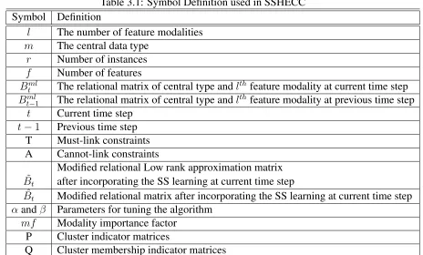
Table 3.1: Symbol Definition used in SSHECC Symbol Definition

l The number of feature modalities

m The central data type

r Number of instances

f Number of features

Bml

t The relational matrix of central type andlthfeature modality at current time step

Bml

t−1 The relational matrix of central type andlthfeature modality at previous time step t Current time step

t−1 Previous time step T Must-link constraints A Cannot-link constraints

Modified relational Low rank approximation matrix

˜

Bt after incorporating the SS learning at current time step

ˆ

Bt Modified relational matrix after incorporating the SS learning at current time step

αandβ Parameters for tuning the algorithm

mf Modality importance factor P Cluster indicator matrices

Q Cluster membership indicator matrices

3.2 SSHECC Algorithm Description

In the heterogeneous relational data environment we havemdata types wherem >1. Each

dataset hasrinstances andffeatures. Each data type is represented asY1

t ={y11,y12,...y1r},

Y_t2={y21, y22,...y2r} , Yt3={y31, y32,...y3r} and Ytm={ym1, ym2,...ymr}. The relationship

between instances ofYm t andY

j

t is measured using the association matrixO mj t ∈R

(nr×nf)

t

where the rows and columns index the instances of the two types. An entry lt signifies

the relation between instances yml and yjt of types Ytm and Y j

t respectively. The data

is analyzed at different time steps denoted by the index t, represented as B_tmj. In the evolutionary settings there are certain situations where the number of instances or features

might differ than the previous time step data matrix. In order to make them equal, we have

four different cases that handle these changes and provide consistent input data matrix.

1. The number of instances in the current time step tis greater than the previous time

(21)

2. The number of instances in the current time steptis less than the previous time step

t−1

3. The number of features in the current time step t is greater than the previous time

stept−1

4. The number of features in the current time stept is less than the previous time step

t−1

In the first case where the number of instances in the current time steptis greater than

the previous time stept−1we take the mean of the features and append them to previous

time step to make the number of instances equal. If we use the deletion approach to make

the number of instances similar in the input matrix we are unable to capture the change

as well as appending some random value instances will shift the clusters drastically and

cluster drift is observed. In the second case where the number of instances in the current

time steptis less than the previous time stept−1we use Colibri to identify the instances

that needs to be removed from thet−1step so as to make the number of instances equal.

In the third scenario if new features are added to the dataset atttime step then to make the

number of features equal in the previous time step datat−1and current time steptwe take

the mean of the instance of the dataset att−1time step and append it to the dataset att−1

time step. If we use the deletion approach to make the number of features equal then we

might not be able to capture the evolving change in the data over a period of time and the

clusters will not be the true representation of the data. In the fourth scenario if the number

of features in the current time step data tis less than the previous time step datat−1we

use the Colibri to identify the features that needs to be deleted from thet−1dataset. In

the evolutionary environment we can provide more emphasis to the current time step data

or the previous time step data by changing the value ofαin the cost function.

The semi-supervised knowledge is incorporated using the pairwise constraints derived

from the given labels on the central data type where the must-link constraints represented

(22)

ymq )∈Ttimplies thatympandymq are belonging to same cluster for the current time step

t, while (ymp,ymq)∈Atimplies thatym andyj are not belonging to the same cluster in the

current time stept. The new association matrix Be

mj

t between Ytm and Y j

t is obtained by

the distance learning matrix Lmj_t for each association matrix O_tmj. Through the distance metric learning and feature selection prior knowledge is integrated into co-clustering for the

current time step t making the must-link data points as close as possible and cannot-link

data points as far as possible.

d(ymp, ymq) =

q

(ymp−ymq)TLmjt (ymp−ymq) (3.1)

The optimization of Lmj_t is equivalent to the generalized semi-supervised linear dis-criminate analysis and is solved iteratively [7]. We compute new association matricesBe_tmj based on the learned distance metrics Lmj_t as shown in the algorithm in section 3.3 Low rank approximation is performed to obtain the sparse representationBbmj_t . Finally, cluster-ing of heterogeneous relational evolvcluster-ing data with the incorporated supervision is achieved

by factorizing matricesBb_tmj. MatrixP_tconsists of the centroid and matrixQ_tcontains the cluster membership indicator, the value indicates the object association with cluster at time

step t. Computing the snapshot quality from equation 3.2, the historic cost is computed

using 3.3 The final cost of the cut given by the equation 3.4

fsq =−

X

16i6j6m

kBb

mj

t −PtmQ mj t P

(j)T

t k2F (3.2)

fhc=

X

16i6j6m

kBb

(mj)

t−1 −P

m t−1Q

mj t−1P

(j)T t−1 k

2

F (3.3)

Jcost =−α.fsq+ (1−α).fhc (3.4)

The final cost of the cut given by the equation 3.4 and the cut is selected to perform

co-clustering of data at time step t in the heterogeneous environment. In the SSHECC

(23)

for every time stept. Later on the number of instances in the current time step data and the

previous time step data are verified and then we compute the sparse matrix using the low

rank approximation. Finally we perform co-clustering on the heterogenous data using the

Non-negative matrix factorization.

As the data is evolving with time the number of clusters might change. Determining the

number of clusters in the evolving data is a challenging task[25]. To address this problem

we are using four different techniques to determine the number of clusters in the data. The

four different techniques are Krzanowski-Lai [19], Davies-Bouldin index[21], Silhouettes

[28] and Calinski-Harabasz index [32],[12]. The number of clusters is determined from

˜

(24)

3.3 SSHECC Algorithm

Algorithm 1Semi-supervised Heterogeneous Evolutionary Co-clustering

Require: A relational matrixB_t(ml) ∈Bnm×nl_for_t₌{₁_,₂_{, ..., S}}

Ensure: P_t(m) ∈ Benm×km (row cluster indicator matrix) and P

(l)

t Bekl×nl (column cluster indicator matrix) andQ(_tml)Bekm×kl (block value matrix)

1: fort= 2,Sdo

2: De_tis the target distance vector consisting of constraintsT_tandA_t,

3: if(ymp, ymq)∈Ttthen

4: de_mp,mq = 0

5: end if

6: if(ymp, ymq)∈Atthen

7: de_mp,mq = 1

8: end if

9: Initial distance metricLml

t is obtained by SS-LDA with constraintsTtandAt

10: Set the number of iterations t=0

11: Bb

(ml)

t =

q

Lml t B

(ml)

t

12: Distance vector with only data points having constraintsD(_tml) 13: mf_topt =argminα||Det−Pl_l₌₁α(ml)D(ml)t||2

14: Let B_t(ml) = α(ml)

b

B_t(ml) and learn the new distance metric L(_tml) by SS-LDA with constraintsTtandAt

15: if ac+1−ac> εthen

16: c=c+ 1

17: repeat above steps

18: else

19: Bb

(ml)

t =B

(ml)

t

20: Exit()

21: end if

(25)

1: fori= 1,ldo 2: ifnrow(Bb

(mi)

t−1 )< nrow(Bb

(mi)

t )then

3: forj =nrow(Bb

(mi)

t−1 ),nrow(Bb

(mi)

t )do

4: insert⇐µ(Bbt)

5: Addinsertinstances toBb_t−1 6: end for

7: end if 8: ifnrow(Bb

(mi)

t−1 )> nrow(Bb

(mi)

t )then

9: Use intermediate results from the Colibri method to get unique and independent subspaces fromBb

(mi)

t−1 equivalent to length ofBb

(mi)

t

10: end if 11: ifncol(Bb

(mi)

t−1 )< ncol(Bb

(mi)

t )then

12: forj =ncol(Bb

(mi)

t−1 ),ncol(Bb

(mi)

t )do

13: insert⇐µ(Bbt)

14: Addinsertfeature toBb_t−1 15: end for

16: end if 17: ifncol(Bb

(mi)

t−1 )> ncol(Bb

(mi)

t )then

18: Use intermediate results from the Colibri method to get unique and independent subspaces fromBb

(mi)

t−1 equivalent to feature length ofBb

(mi)

t

19: end if

{UseColibri−Dmethod to obtain Low Rank approximation ofBbt−1withBbt}

20: tempBb

(mi)

t−1 ⇐Colibri−D(Bb

(mi)

t−1 ,Bb

(mi)

t )

21: B˜_t(mi) ⇐α·Bb

(mi)

t + (1−α)·tempBb

(mi)

t−1 22: end for

23: Estimate number of clusters inB˜_t(mi)

24: Obtain the clustering using the following rules by applying recursive onB˜(_tmi) 25: Subject to the constraints∀ab : P

(m)

Sab ≥ 0andP

(i)

Sab ≥ 0,wherek · kdenote Frobenius

matrix norm,P_S(m) ∈Ben×k, Q

(mi)

S ∈Bek×l, P

(i)

S ∈Bel×m, k nandl m.

P₍(_Sm₎₍)_ab₎ ⇐P₍(_Sm₎₍)_ab₎

Pl

i=1((

PS

t=1α(1−α)

S−t_·_B_˜(mi)

t )P

(i)T (S) Q

(mi)T (S) )ab

Pl

i=1(P (m) (S) Q

(mi) (S) P

(i) (S)P

(i)T

(S) Q (mi)T

(S) )ab

(3.5)

P₍(_Si)₎₍_ab₎⇐P₍(_Si)₎₍_ab₎(Q (mi)T

(S) P (m)T

(S) (

PS

t=1α(1−α)S

−t_·_B˜(mi) t ))ab

Pl

i=1(Q (mi)T

(S) P (m)T

(S) P (m) (S) Q

(mi) (S) P

(i) (S))ab

(3.6)

Q(₍mi_S₎₍)_ab₎ ⇐Q(₍mi_S₎₍)_ab₎(P (m)T

(S) (

PS

t=1α(1−α)S

−t_·_B_˜(mi) t )P

(i)T

(S) )ab

Pl

i=1(P (m)T

(S) P (m) (S) Q

(mi) (S) P

(i) (S)P

(i)T

(S) )ab

(26)

4. Experiments

This chapter explains the data pre-processing steps performed on the datasets used in

ex-perimentation and the different experiments performed to validate the proposed SSHECC

algorithm described in the previous section. We have used publicly available datasets and a

synthetic dataset to validate the SSHECC Algorithm. The real datasets consist of the web

service community dataset[29],[36] and the image dataset[6],[27]. The synthetic dataset

is generated using the Bernoulli processes [7]. All the datasets have been preprocessed,

cleaned and evolved so that we have the data in the required format forming a star structure

and multiple time steps.

4.1 Dataset preparation

4.1.1 Image Dataset

An image data set is created for the experimentation, consisting of 4700 images which are

selected from 47 categories of images where each category consists of 100 images. The

images belong to animal, automobiles, hairstyles, waterfalls, landscape, etc. We are

ex-tracting the 45 color features, 42 texture features from the images as well as incorporating

the user feedback in the form of log features. The color features includes color channels

and the texture feature includes Gabor wavelength based texture, edge detection histogram

and edge direction coherence vector. The image−log relational matrix is generated

de-pending on the number of image categories selected, the number of images selected per

category and number of logs for each category. For each category of image randomly few

of the images are selected and marked 1. Multiple logs for each category of images are

(27)

in each category. Based on the extracted visual features we build three rational matrices.

Theimage−color,image−textureand theimage−logwhich simulated the

heteroge-nous environment for the experiments. Each element in the matrices is normalized into the

range of [0,1]. Semi-supervised knowledge is provided and co-clustering is then performed

on the images, color features, texture features and log features simultaneously. The image

dataset simulates the heterogeneous data environment as shown in figure 4.1. Where

im-age is the central data type and is connected by the color features, texture features and log

features forming a heterogeneous star structured schema. We are placing the constraints

on the images which is the central data type in the image dataset experiment. Constraints

are placed on the current time step data. To simulate the heterogeneous evolved data

envi-ronment for the experiment purpose. The data is evolved from time step t0 tot7, where at

every time step the instances or features are evolved such as some number of instances are

shifted from one cluster to another, some of new instances are added, some instances are

removed.

4.1.2 Web service Dataset

The WSDL document that contains the web service information which is used to extract the

terms, services and operations that the web service is composed of. Different techniques

like tokenization , portering and stemming are used to extract the required information to

create the web service dataset. As shown in figure 4.1 a. the web services dataset consists

of two relational matrices one isterms−operationsand the second isterms−services.

Theterms−operationsmatrix consists of 384 terms and 72 operations. In theterms−

services matrix we have 384 terms and 97 services. Terms is the central data type in

this dataset. Semi-supervised knowledge is incorporated for co-clustering by placing the

constraints on the central type which is terms in this case. The number of row clusters and

column clusters is five. Terms belong to various categories like communication, education,

food, medical and travel. This simulates the tri-type of data where terms from the central

(28)

[image:28.612.95.548.109.394.2]

Figure 4.1: (a).Web service and (b). Image datasets forming a star structure schema where, (a). The terms forms the central type and is connected to service and operations. (b). The image forms cental type and is connected to texture feature, Gabor feature and user logs

4.1.3 Synthetic Dataset

The synthetic data is generated using the Bernoulli processes. Two different types of

syn-thetic datasets were generated from the same process where the numbers of instances,

fea-tures, number of row clusters and column cluster were changed.In the first set of synthetic

datasets, the central type is connected to three other types of data. The dimensions of the

first relation R11 has 400 instances and 200 features.The relation R12 is having 400

in-stances and 100 features. The last relation R13 is having 400 instances and 60 features.

There are 3row clusters and 2column clusters in R11, R12 andR13. The data is evolved

from time step t0 tot7. Such that at each time step either the instances are evolved or

(29)

new features or instances, or deletion of instances or features. In the second set of synthetic

dataset, the central type is connected to three other types of data the dimensions of the first

relationR11has1000instances and200features. The relationR12is having1000instances

and100features. The last relationR13is having1000instances and60features. There are

5row clusters and2column clusters inR11,R12andR13.

The data is evolved in both the dataset from time stept0 tot7 such that at each time

step either the instances are evolved or features are evolved. The evolving step consists

of change of instances or features, addition of new features or instances, or deletion of

instances or features.

4.2 Experiments

The SSHECC algorithm’s accuracy is validated using the multiple set of experiments

per-formed on the two real datasets and a synthetic dataset. Real world datasets are selected

from different fields such as the web services dataset[29] and image dataset [27]. The

syn-thetic data set is generated using the Bernoulli process [7] as mentioned in the data pre

processing steps.

The accuracy is measured in terms of micro-accuracy [7]. The co-clustering accuracy is

measured on all the datasets by varying the number of must-link and cannot-link constraints

on the central data. The co-clustering accuracy is measured by changing the αparameters

and changing the percentages of instances and features that are evolved from time step t0

tot7, and by varying the constraints percentage at every time step.

Figure 4.2 shows how the algorithm detects the number of clusters in the underlying

data. The data is evolved at each time step. As mentioned earlier we are using four different

techniques to calculate the number of clusters and then the mode is taken, so that we get

the most accurate number of clusters present in the data.

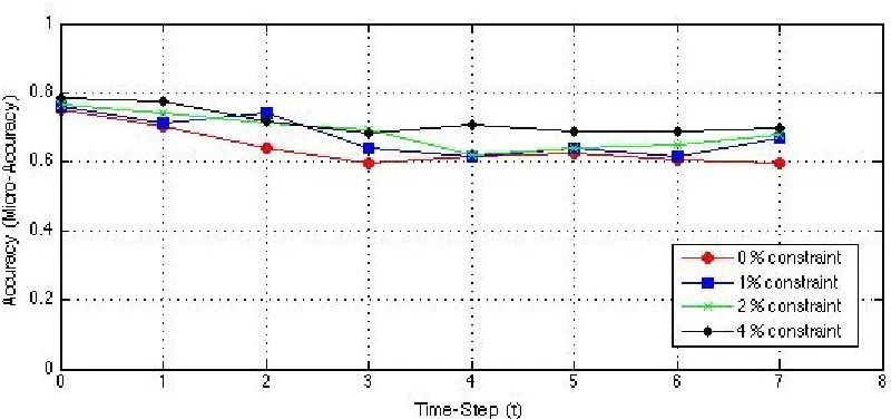
Figure 4.3 is the plot of co-clustering accuracy of SSHECC on the evolving data for

(30)

[image:30.612.136.488.105.430.2]

Figure 4.2: Detecting the number of clusters in the current time step data t using Krzanowski-Lai, Davies-Bouldin index, Silhouettes and Calinski-Harabasz index tech-niques

constraints. The value ofαis 0.8 and at current time step ist0. At time stept1, 10 percent of

the instances are shifted from one cluster to another. In the next time stept2, 10 percent of

the instances are added to a cluster, at time stept3, 5 percent of the instances are removed.

We can see the co-clustering accuracy is reduced at this time step. But at the next time

step i.e. t4, 10 percent of features are shifted from one cluster to another the algorithms

ability to perform consistent co-clustering even as the data evolves can be observed. Also

as the percentage of the constraints is increased the co-clustering accuracy is improved as

(31)

[image:31.612.111.511.127.315.2]

Figure 4.3: Semi-supervised co-clustering accuracy is measured by placing 0, 1, 2 and 4 percent constraint on evolving web service dataset from time step t0 to t7 where the

numbers of instances features are shifted, added or removed from clusters.

on the current data at every time step. As we can see the overall accuracy improves when

constraints are placed. The lowest accuracy is when we perform co-clustering without any

semi-supervised knowledge. i.e. 0 percent constraint.

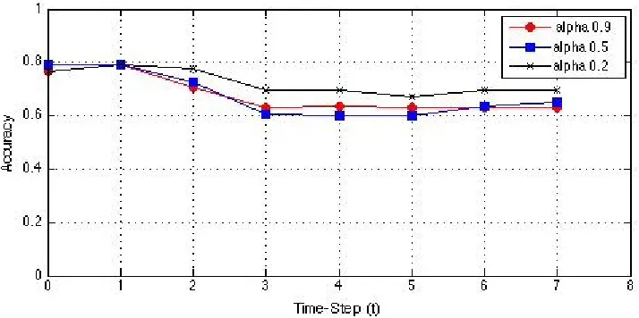
Figure 4.4 shows the co-clustering accuracy of the SSHECC on the evolving web

ser-vice data where the value ofαis set to 0.9, 0.5 and 0.2 to measure if the value ofαimpacts

accuracy. When the value ofαis 0.9 it means more value is given to the current time step

data while performing clustering with respect to historic data. The value ofα= 0.2 means

more importance is given to the historic data while clustering the current time step data and

the current time step data will be clustered according to the historic clusters. The value of

α= 0.5 means equal weights are assigned to the current time step data and the historic time

step data to obtain the cluster.

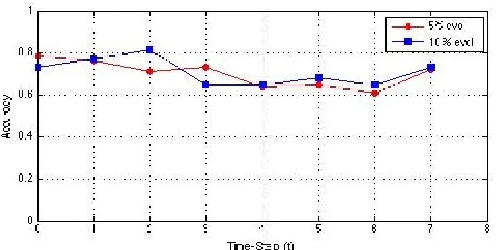
Figure 4.5 shows that only 1 percent constraint were placed on the evolving web service

(32)

[image:32.612.131.488.112.290.2]

Figure 4.4: Measuring the semi-supervised co-clustering accuracy by varying the value of

αwhile keeping the constraint percentage constant on the web service dataset

that are evolved. In the first set of evolved data only 5 percent of the instances were evolved

at each time steptand in the second set the data was evolved by 10 percent at each time step

t. As we see the co-clustering accuracy is almost similar in both the runs. This implies that

the algorithm performs well and provides consistent results and is capable of handling the

changes in the evolving data, even when new instances or features are added or removed or

shifted from one cluster to another. This experiment models the real word scenario where

the data is evolving and the percentage of instances that are added or removed or shifted

can change.

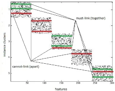
Figure 4.6 shows the co-clustering snapshot of the image and the log feature data at

time stept where we have 450 instances clustered into 5 different clusters represented on

the Y-axis and 60 logs per image category so the total number of features is 300

repre-sented by the X-axis. We are generating the constraints on the instances of central type

i.e. images in this case to embed the semi-supervised knowledge. The semi-supervised

(33)

[image:33.612.129.488.128.309.2]

Figure 4.5: Comparing the results of SSHECC when the percentage of evolved instances change keeping the constraints andαconstant on the web service dataset

must-link (together) constraint. Such that instances belonging to the same cluster are

to-gether and the red lines indicate the instances belonging to the different clusters should not

be together thereby maximizing the distance between those two data points. As we can see

the instances within the cluster C1, C3 and C5 are together whereas the instance in C1 and

instance in C2, C2 and C3 , C4 and C5 are having cannot link (apart) constraint since they

do not belong to the same cluster.

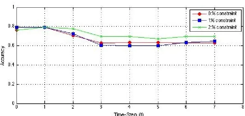
Figure 4.7 shows the co-clustering accuracy of the SSHECC algorithm on the image

data which is evolved from time t0 tot7 with constant constraint percentage at every run.

The image dataset consists of images belonging to 47 categories and each category is

hav-ing 100 images. Multiple numbers of experiments are performed by varyhav-ing the number of

images selected from each category. We are randomly selecting 5 categories of images and

90 images in each category, the value ofαis set to 0.8. The percentages of evolved instance

(34)

[image:34.612.125.493.111.404.2]

Figure 4.6: Visual representation of must-link and cannot-link constraint on the image and the user log dataset at time steptconsisting of 5 row and column clusters. The constraints are placed on the central type data. i.e. images represented by green and red lines

randomly selecting different image categories and the rest of the parameters we kept the

same to observe that the co-clustering accuracy is not impacted by different categories of

images. The observed results were consistent. From the above figure it is clear that the

co-clustering accuracy increases when the percentage of the constraints increases. This

validates our assumptions that SSHECC performs well when the percentage of constraints

is increased on the images. SSHECC performs co-clustering efficiently on different image

categories and accuracy is consistent and independent of the image categories.

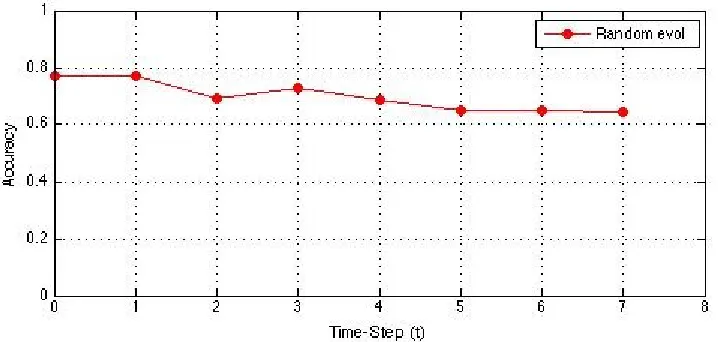
In figure 4.8 only the instances are evolved in a random fashion on the web service

(35)

[image:35.612.109.509.124.313.2]

Figure 4.7: Semi-supervised co-clustering accuracy is measured by placing 0, 1 and 2 percent constraint on the evolving image dataset from time stept0tot7where the numbers

of instances features are shifted, added or removed from clusters.

accuracy vs the time step t is plotted as we can see even if the new instances are added,

deleted or shifted from one cluster to another to another the SSHECC algorithm performs

efficient co-clustering as measured by the co-clustering accuracy. This implies that the

SSHECC is capable of efficiently handling the evolving changes and performing

consis-tently. This environment simulates that random events happen in the real world situation

where features remain constant and only the instances changes.

Figure 4.9 represents the co-clustering accuracy on evolving synthetic dataset. The

SSHECC algorithm was run for different percentage of constraints and accuracy is

mea-sured. The value ofαis set to 0.8 and the SSHECC is executed for different percentage of

constraints. The evolving percentage of instances is set between 10 to 15. The new

con-straints are generated for every time step. In figure 4.9 at timet112 percent of the instances

(36)

[image:36.612.131.490.111.282.2]

Figure 4.8: Measuring the semi-supervised co-clustering accuracy on image dataset where instances are evolved randomly keeping the percentage constraint andαconstant

of the instances are removed. Similarly at time stept4,t5,t6andt77 percent of features are

shifted, 4 percent features are removed and 10 percent features are removed respectively.

After conducting multiple experiments on web service, image and synthetic datasets we

observed that as the semi-supervised knowledge is provided to the co-clustering algorithm

on the evolving data, the co-clustering accuracy increases for all the datasets. However the

percent increase in the co-clustering accuracy as the percentage of constraints increases is

different for all the datasets as well as how the data is evolved. The SSHECC algorithm

can handle changes in the evolving data and perform consistently. Also the SSHECC can

handle random evolving of the data. This validates our assumption that SSHECC algorithm

performs co-clustering efficiently and can be used in solving the real world problems where

the percentage of the labeled instances is small, also the co-clustering accuracy increases

(37)

[image:37.612.134.488.278.459.2]

Figure 4.9: Semi-supervised co-clustering accuracy is measured by placing 0, 1, 3 and 5 percent constraint on the evolving synthetic dataset from time step t0 to t7 where the

(38)

5. Conclusion

I have presented a novel algorithm to perform semi-supervised co-clustering of

hetero-geneous evolving data (SSHECC). The semi-supervised knowledge is incorporated in the

evolving data by placing the must-link and cannot-link constraints on the central data type

of the current time step data. The new relational matrix is then reduced into a sparse

representation using the Colibri approach and finally co-clustering is performed using the

non-negative matrix factorization technique. The experimental results in the previous

sec-tion on the real datasets as well as synthetic dataset have shown increased co-clustering

accuracy as the percentage of semi-supervised knowledge is increased. Further research of

incorporating the semi-supervised knowledge using different techniques as well as a new

heuristics in order to select the instances on which the must-link and cannot-link constraints

(39)

6. Acknowledgments

Thanks to Professor Rege for mentoring me during my Masters and also providing me the

knowledge of Data Mining as well as guiding me through the thesis. Thanks to the staff

members of the computer science department at Rochester Institute of Technology, all the

committee members for serving on my committee. Thanks to Amit Salunke for helping me

in pre-processing image dataset. Thanks to Hanghang Tong, Spiros Papadimitriou, Jimeng

Sun, Philip Yu and Christos Faloutsos for making Colibri [33], implementation as well as

to Yanhua Chen, Lijun Wang and Ming Dong for making semi-supervised distance learning

(40)

Bibliography

[1] E.M. Airoldi, D.M. Blei, S.E. Fienberg, and E.P. Xing. Mixed membership stochastic blockmodels. The Journal of Machine Learning Research, 9:1981–2014, 2008.

[2] Arindam Banerjee, Inderjit Dhillon, Joydeep Ghosh, Srujana Merugu, and Dharmen-dra S. Modha. A generalized maximum entropy approach to bregman co-clustering and matrix approximation. J. Mach. Learn. Res., 8:1919–1986, December 2007.

[3] R. Bekkerman and M. Sahami. Semi-supervised clustering using combinatorial mrfs. InICML-06 Workshop on Learning in Structured Output Spaces, 2006.

[4] Michael W. Berry, Shakhina A. Pulatova, and G. W. Stewart. Algorithm 844: Com-puting sparse reduced-rank approximations to sparse matrices. ACM Trans. Math. Softw., 31:252–269, June 2005.

[5] Deepayan Chakrabarti, Ravi Kumar, and Andrew Tomkins. Evolutionary clustering.

In Proceedings of the 12th ACM SIGKDD international conference on Knowledge

discovery and data mining, KDD ’06, pages 554–560, New York, NY, USA, 2006.

ACM.

[6] Yanhua Chen, Manjeet Rege, Ming Dong, and Jing Hua. Non-negative matrix factor-ization for semi-supervised data clustering. Knowl. Inf. Syst., 17:355–379, November 2008.

[7] Yanhua Chen, Lijun Wang, and Ming Dong. Non-negative matrix factorization for semisupervised heterogeneous data coclustering. IEEE Trans. on Knowl. and Data Eng., 22:1459–1474, October 2010.

[8] Yun Chi, Xiaodan Song, Dengyong Zhou, Koji Hino, and Belle L. Tseng. Evolu-tionary spectral clustering by incorporating temporal smoothness. InProceedings of the 13th ACM SIGKDD international conference on Knowledge discovery and data

(41)

[9] Inderjit S. Dhillon, Subramanyam Mallela, and Dharmendra S. Modha. Information-theoretic co-clustering. InProceedings of the ninth ACM SIGKDD international con-ference on Knowledge discovery and data mining, KDD ’03, pages 89–98, New York, NY, USA, 2003. ACM.

[10] Petros Drineas, Ravi Kannan, Michael W. Mahoney, and Let A. Fast monte carlo algorithms for matrices iii: Computing a compressed approximate matrix decompo-sition. SIAM Journal on Computing, 36:2006, 2004.

[11] Bin Gao, Tie-Yan Liu, Xin Zheng, Qian-Sheng Cheng, and Wei-Ying Ma. Consistent bipartite graph partitioning for star-structured high-order heterogeneous data co-clustering. InProceedings of the eleventh ACM SIGKDD international conference on

Knowledge discovery in data mining, KDD ’05, pages 41–50, New York, NY, USA,

2005. ACM.

[12] John A. Hartigan. Clustering Algorithms. John Wiley & Sons, Inc., New York, NY, USA, 99th edition, 1975.

[13] T. Hofmann. Probabilistic latent semantic indexing. In Proceedings of the 22nd annual international ACM SIGIR conference on Research and development in infor-mation retrieval, pages 50–57. ACM, 1999.

[14] Yi Hong, Sam Kwong, Hanli Wang, Qingsheng Ren, and Yuchou Chang. Probabilistic and graphical model based genetic algorithm driven clustering with instance-level constraints. InEvolutionary Computation, 2008. CEC 2008. (IEEE World Congress on Computational Intelligence). IEEE Congress on, pages 322 –329, june 2008.

[15] A. K. Jain, M. N. Murty, and P. J. Flynn. Data clustering: a review. ACM Comput.

Surv., 31(3):264–323, September 1999.

[16] Anil K. Jain. Data clustering: 50 years beyond k-means. Pattern Recogn. Lett., 31(8):651–666, June 2010.

[17] Xiang Ji and Wei Xu. Document clustering with prior knowledge. InProceedings of

the 29th annual international ACM SIGIR conference on Research and development

in information retrieval, SIGIR ’06, pages 405–412, New York, NY, USA, 2006.

(42)

[18] C. Kemp, J.B. Tenenbaum, T.L. Griffiths, T. Yamada, and N. Ueda. Learning systems of concepts with an infinite relational model. InProceedings of the national confer-ence on artificial intelligconfer-ence, volume 21, page 381. Menlo Park, CA; Cambridge, MA; London; AAAI Press; MIT Press; 1999, 2006.

[19] W.J. Krzanowski and YT Lai. A criterion for determining the number of groups in a data set using sum-of-squares clustering. Biometrics, pages 23–34, 1988.

[20] Brian Kulis, Sugato Basu, Inderjit Dhillon, and Raymond Mooney. Semi-supervised graph clustering: a kernel approach, 2008.

[21] David D. Lewis, Yiming Yang, Tony G. Rose, and Fan Li. Rcv1: A new bench-mark collection for text categorization research. J. Mach. Learn. Res., 5:361–397, December 2004.

[22] Bo Long, Zhongfei (Mark) Zhang, and Philip S. Yu. Co-clustering by block value de-composition. InProceedings of the eleventh ACM SIGKDD international conference

on Knowledge discovery in data mining, KDD ’05, pages 635–640, New York, NY,

USA, 2005. ACM.

[23] X. Liu N. Green, M. Rege and R. Bailey. Evolutionary spectral co-clustering. IEEE Trans. on Knowl. and Data Eng., 2011.

[24] W. Pedrycz and Keun-Chang Kwak. The development of incremental models. Fuzzy

Systems, IEEE Transactions on, 15(3):507 –518, june 2007.

[25] Yi Peng, Yong Zhang, Gang Kou, and Yong Shi. A multicriteria decision making approach for estimating the number of clusters in a data set. PLoS ONE, 7(7):e41713, 07 2012.

[26] H. Prehn and G. Sommer. An adaptive classification algorithm using robust incre-mental clustering. InPattern Recognition, 2006. ICPR 2006. 18th International

Con-ference on, volume 1, pages 896 –899, 0-0 2006.

[27] Manjeet Rege, Ming Dong, and Farshad Fotouhi. Co-clustering documents and words using bipartite isoperimetric graph partitioning. InProceedings of the Sixth

Interna-tional Conference on Data Mining, ICDM ’06, pages 532–541, Washington, DC,

(43)

[28] Peter Rousseeuw. Silhouettes: a graphical aid to the interpretation and validation of cluster analysis. J. Comput. Appl. Math., 20(1):53–65, November 1987.

[29] Amit Salunke, Minh Nguyen, Xumin Liu, and Manjeet Rege. Web service discovery using semi-supervised block value decomposition. InIRI, pages 36–41, 2011.

[30] H. Shan and A. Banerjee. Bayesian co-clustering. InData Mining, 2008. ICDM’08. Eighth IEEE International Conference on, pages 530–539. IEEE, 2008.

[31] Jimeng Sun, Yinglian Xie, Hui Zhang, and Christos Faloutsos. Less is more: Compact matrix decomposition for large sparse graphs. In In Proc. SIAM Intl. Conf. Data Mining, 2007.

[32] K. Tasdemir and E. Merenyi. A new cluster validity index for prototype based clus-tering algorithms based on inter- and intra-cluster density. In In Proc. International Joint Conference on Neural Networks (IJCNN 2007), 2007.

[33] Hanghang Tong, Spiros Papadimitriou, Jimeng Sun, Philip S. Yu, and Christos Falout-sos. Colibri: fast mining of large static and dynamic graphs. InProceeding of the 14th

ACM SIGKDD international conference on Knowledge discovery and data mining,

KDD ’08, pages 686–694, New York, NY, USA, 2008. ACM.

[34] Lijun Wang, Manjeet Rege, Ming Dong, and Yongsheng Ding. Low-rank kernel matrix factorization for large scale evolutionary clustering. IEEE Transactions on

Knowledge and Data Engineering, 99(PrePrints), 2010.

[35] Eric P. Xing, Andrew Y. Ng, Michael I. Jordan, and Stuart Russell. Distance metric learning, with application to clustering with side-information. InAdvances in Neural

Information Processing Systems 15, pages 505–512. MIT Press, 2002.

[36] Qi Yu and Manjeet Rege. On service community learning: A co-clustering approach.