City, University of London Institutional Repository
Citation
:
Andrienko, N., Andrienko, G., Stange, H., Liebig, T. & Hecker, D. (2012). Visual Analytics for Understanding Spatial Situations from Episodic Movement Data. Künstliche Intelligenz, 26(3), pp. 241-251. doi: 10.1007/s13218-This is the accepted version of the paper.
This version of the publication may differ from the final published
version.
Permanent repository link:
http://openaccess.city.ac.uk/13256/Link to published version
:
http://dx.doi.org/10.1007/s13218-Copyright and reuse:
City Research Online aims to make research
outputs of City, University of London available to a wider audience.
Copyright and Moral Rights remain with the author(s) and/or copyright
holders. URLs from City Research Online may be freely distributed and
linked to.
City Research Online: http://openaccess.city.ac.uk/ [email protected]
Visual Analytics for Understanding Spatial
Situations from Episodic Movement Data
Natalia Andrienko, Gennady Andrienko, Hendrik Stange, Thomas Liebig, Dirk Hecker
Fraunhofer Institute IAIS (Intelligent Analysis and Information Systems), Schloss Birlinghoven, 53754, Sankt Augustin, Germany
Abstract
Continuing advances in modern data acquisition techniques result in rapidly growing amounts of geo-referenced data about moving objects and in emergence of new data types. We define episodic movement data as a new complex data type to be considered in the research fields relevant to data analysis. In episodic movement data, position measurements may be separated by large time gaps, in which the positions of the moving objects are unknown and cannot be reliably reconstructed. Many of the existing methods for movement analysis are designed for data with fine temporal resolution and cannot be applied to discontinuous trajectories. We present an approach utilizing Visual Analytics methods to explore and understand the temporal variation of spatial situations derived from episodic movement data by means of spatio-temporal aggregation. The situations are defined in terms of the presence of moving objects in different places and in terms of flows (collective movements) among the places. The approach, which combines interactive visual displays with clustering of the spatial situations, is presented by example of a real dataset collected by Bluetooth sensors.
Introduction
The popularity of cellular phones and advances in information and sensor technologies lead the way towards new location recording techniques and thus new types of movement data. ‘Episodic movement data’ refers to data about spatial positions of moving objects where the time intervals between the
Location based: Positions of objects are recorded only when they come into
the range of static sensors. The temporal resolution of the collected data depends on the coverage and density of the spatial distribution of the sensors.
Activity based: Positions of objects are recorded only at the times when they
perform certain activities, for example, call by mobile phones, pay by credit cards or send posts to a community website.
Device based: Positions are measured and recorded by mobile devices
attached to the objects but this cannot be done sufficiently frequently, for example, due to the limited battery lives of the devices i.e. when tracking movements of wild animals.
Irrespective of the collection method we can identify three types of uncertainty. First, the common type of uncertainty in any episodic movement data is the lack of information about the spatial positions of the objects between the recorded positions (continuity), which is caused by large time intervals between the recordings and by missed recordings. Second, a frequently occurring type of uncertainty is imprecision of the recorded positions (accuracy). Thus, a sensor may detect an object within its range but may not be able to determine the exact coordinates of the objects. For a mobile phone call, the localization precision may be the range of a certain antenna but not an exact point in space. Due to these uncertainties, episodic movement data cannot be represented as continuous trajectories, i.e., lines in the spatio-temporal continuum where known (measured) positions are linked by straight or curved segments. Third, the number of recorded objects (coverage) may also be uncertain due to the usage of a service or due to the utilized sensor technology. For example, one individual may carry two or more devices with Bluetooth transceivers, which will be registered by Bluetooth sensors as independent objects. On the other hand, the sensors only capture devices with activated Bluetooth services. The activation status may change while a device carrier moves from one sensor to another.
(these computations also assume that the positions are precise). The same holds for summarisation of movement data in the form of density or vector fields. Mining methods for finding patterns of relative or collective movement of two or more objects (e.g. meeting or flocking) also require fine-resolution data. Since many of the existing methods are not applicable to episodic movement data, there is a need in finding suitable approaches to analysing this kind of data.
Due to the uncertainties, episodic data are usually not suitable for studying the movement behaviours of individual objects. In order to overcome these
shortcomings, we suggest aggregating of many individual tracks to compensate for missing data and uncertainties in the spatial and temporal coverage.
By example of episodic movement data, this paper motivates the utilisation of visual and computational methods to analysing complex data. Visual analytics strives at multiplying the analytical power of both human and computer by finding effective ways to combine interactive visual techniques with algorithms for
computational data analysis (Keim et al. 2008). The key role of the visual techniques is to enable and promote human understanding of the data.
Particularly, visual analytics can help in understanding the data for data mining tasks, such as distributions, features, clusters, patterns. Visual analytics
approaches are applied to data and problems for which there are (yet) no purely automatic methods to deal with. By enabling human understanding, reasoning, and use of prior knowledge and experiences, visual analytic can help the analyst to find suitable ways for data analysis and problem solving, which, possibly, can later be fully or partly automated. Thus, visual analytics can drive the
development and adaption of learning and mining algorithms.
In the next section, we describe aggregation of episodic movement data and define the analysis tasks in which the aggregated data can be used. Then, after discussing the relevant literature, we present our visual analytics methods and tools using an example of episodic movement data collected by Bluetooth sensors.
Spatio-temporal aggregation
Episodic movement data consist of records including the following components: object identifier ok, spatial position pi, time t, and, possibly, other attributes. The
and dimension in space. A chronologically ordered sequence of positions of one moving object can be regarded as an abstract trajectory which is spatially and temporally discontinuous.
For temporal aggregation of the data, time is divided into intervals. Depending on the application and analysis goals, the analyst may consider time as a line (i.e. linearly ordered set of moments) or as a cycle, e.g., daily, weekly, or yearly. Accordingly, the time intervals are defined on the line or within the chosen cycle. For spatial aggregation, it is necessary to define a finite set of places visited by the moving objects. Two different cases need to be distinguished:
1. The object positions in the data are limited to a finite set of predefined positions, such as positions of sensors or cells of a mobile phone network. 2. The object positions in the data are arbitrary. This is the case when the
positions are received from mobile devices worn by the objects and capable of measuring absolute spatial positions, such as GPS devices.
In the first case, the different positions from the data can be directly used as places for the aggregation. To do analysis at a higher spatial scale, the analyst may group neighbouring positions and define places as convex hulls or spatial buffers or Voronoi polygons around the groups.
On the basis of the defined set of places P, each trajectory is represented by a sequence of visits v1, v2, …, vn of places from P. A visit vi is a tuple <ok, pi, tstart,
tend>, where ok is the moving object, piP is a place, tstart is the starting time of the
visit, and tend is the ending time. Complementarily to this, each trajectory is also
represented by a sequence of moves m1, m2,…, mn-1, where a move mi is a tuple
<ok, pi, pi+1, t0, tfin> describing the transition from place pi to place pi+1. Here t0 is
the time moment when the move began (it equals tend of the visit vi of the place pi)
and tfin is the time moment when the move finished (it equals tstart of the visit vi+1
of the place pi+1). It should be borne in mind that consecutively visited places pi
and pi+1 in a discontinuous trajectory are not necessarily neighbours in space.
Having a dual representation of trajectories, as sequences of visits and as sequences of moves, the data can be aggregated in two complementary ways. First, for each place pi and time interval t, the visits of this place in this interval
are aggregated, i.e., the tuples <ok, pi, tstart, tend> where t: tstart≤ t ≤ tend & tt.
The count of the visits and the count of different visitors (ok) are computed. If the
original data records include additional attributes, various statistics of these attributes can also be computed, such as minimum, maximum, average, median, etc. Hence, each place is characterized by two or more time series of aggregate values: counts of visits, counts of visitors, and, possibly, additional statistics by the time intervals.
The second way of aggregation is applied to links, i.e., pairs of places <pi, pj>
such that there is at least one move from pi to pj. For each link <pi, pj> and time
interval t, the moves from pi to pj in this interval are aggregated, i.e., the tuples
<ok, pi, pj, t0, tfin> where tfint (which means that only the moves that finished
within the interval t are included). The count of the moves and the count of different objects that moved (ok) are computed. If the original data include
additional attributes, it is also possible to compute changes of the attribute values from t0 to tfin and then aggregate the changes by computing various statistics.
Hence, each link is characterized by two or more time series of aggregate values: counts of moves, counts of moving objects, and, possibly, additional statistics of changes by the time intervals.
Investigation of the presence of moving objects in different places and the temporal variation of the presence. The presence is expressed by the counts of visits and visitors in the places.
Investigation of the flows (aggregate movements) of objects among different places and the temporal variation of the flows. The flows are represented by the counts of moves and moving objects for the links. These aggregate attributes are often referred to as flow magnitudes.
In both classes of tasks, the aggregated data can be viewed in two ways. Obviously, the data can be viewed as time series associated with the places or links. The analyst can investigate the individual time series or groups of time series (e.g., clusters of similar time series) using existing methods for time series analysis. On the other hand, the data can be viewed as a sequence of spatial situations associated with the time intervals. A spatial situation is the distribution
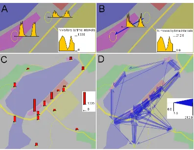
[image:7.595.131.527.377.684.2]of the object presence or flows over the whole territory during a time interval. The different views on aggregated movement data are illustrated by maps in Figure 1.
Figure 1. Different views on aggregated movement data. A, B: Time series associated with places (A) and links (B). C, D: spatial situations in terms of presence (C) and flows (D).
proportional to the values in different time intervals. The places themselves are represented by ellipses and the link by a special symbol (further referred to as flow symbol) looking as a half of an arrow and pointing in the direction of the
movement. Such half-arrow symbols are used to be able to represent flows between two places in two opposite directions. In Figure 1C and 1D, spatial situations in a selected time interval in terms of presence (C) and flows (D) are shown. The presence is shown by proportional heights of the bars drawn in the places and the flow magnitudes by proportional widths of the flow symbols. A map where aggregated movement is shown by flow symbols is called flow map
(Kraak and Ormeling 2003). It should be considered that by convention flow symbols (e.g. arrows) represent only counts of items or amounts of goods moving between some places but not the routes of the movement.
In Figure 1D there are many intersections among the flow symbols, which clutter the display. This is a consequence of the discontinuity of the original trajectories, where consecutive recorded positions may be quite distant in space.
For the brevity sake, we shall call spatial situations in terms of presence ‘presence situations’ and spatial situations in terms of flows ‘flow situations’.
Related works
Analysis of movement data is now a hot topic in the research areas of machine learning, databases, and visual analytics. However, there are only a few works that address episodic movement data. The use of spatio-temporal aggregation can be seen in papers by Jankowski et al. (2010) and Wood et al. (2011). Vrotsou et al. (2011) consider aggregated movement data as a weighted directed graph where vertices are the places and arcs are the flows. Various centrality measures are computed for the graph vertices; this can be done by the time intervals. The centrality measures may be a valuable addition to the presence indicators and other place-related statistics. Aggregated data referring to places are visualised and analysed as usual spatially referenced time series. The values attained in the places in different time moments are visualised on animated maps. The time series are also represented by lines on line charts (a.k.a. time graphs).
varying their degree of opacity, removing the middle parts of the symbols (e.g. Boyandin et al. 2010), and edge bundling, i.e., representing multiple links by a single complex symbol (e.g. Phan et al. 2005).
Besides flow maps, flows have been visualised in the form of origin-destination (OD) matrices (e.g. Guo et al. 2006), which are free from occlusions but lack spatial context. Guo et al. (2006) also use multiple small maps each showing flows to/from one particular place. The maps are arranged similarly to the
geographical positions of the respective places. Wood et al. (2010, 2011) devised an algorithm to generate so called OD maps, in which multiple OD matrices are arranged according to the geographic positions of the places. This approach can convey spatial but not temporal patterns of the movement.
Apart from the aggregation-based techniques, a few other approaches have been applied to episodic movement data. Bak et al. (2009) represent each visit of a place by a coloured pixel (tiny rectangle) positioned on a map close to the place location. The pixels are coloured according to the time of the visit. The
arrangement of the pixels produces a kind of place-based aggregation, which is visual rather than computational. The flows between the places are not shown. Andrienko et al. (2011) generalise discontinuous trajectories and then find clusters of trajectories according to the similarity of the routes, i.e., sequences of the visited places.
Investigation of temporal variation of spatial situations is not well supported by existing tools. It is difficult and time consuming to investigate the situations in all time moments one by one or to compare each situation with all others. We suggest an approach based on clustering of spatial situations. Earlier Andrienko et al. (2010) applied clustering to presence situations derived from quasi-continuous trajectories but did not deal with flow situations. Examination and comparison of the clusters was done using static images of individual situations. We advance this technology by summarizing clusters and representing them on interactive maps and enabling computation and visualization of differences between the clusters.
Example dataset
places, entrances to the area and to spectators’ tribunes, the information centre, places with shops and restaurants, and other attractions. The data were collected during two consecutive days, Saturday and Sunday. The devices having Bluetooth transceivers, such as mobile phones and digital cameras, which were carried by the visitors coming close to the sensors, were anonymously registered by the sensors. In total, the sensors registered 12,185 different devices and made 792,694 time-stamped records. After cleaning, we have built from these records
discontinuous trajectories reflecting the movements of 9,226 device carriers, which is about 15% of the total number of the area visitors in these two days. It is reasonable to assume that the people from the sample behaved similarly to the other visitors. The procedure of data collection, cleaning, and preparation for the analysis is described by Stange et al. (2011).
The data have been aggregated spatially by the POIs and temporally by 30-minutes intervals. For the 17 places, there are 276 links.
Analysis of presence
Clustering of spatial situations in different time intervals by similarity reduces the workload of the analyst: instead of exploring each situation separately, it is possible to investigate groups of similar situations. Besides, an appropriate visual representation of the clustering results can disclose the patterns of the temporal variation: whether similar spatial situations occur adjacently or closely in time or may be separated by large time gaps, whether the changes between successive intervals are smooth or abrupt, whether the variation is periodic, etc.
second, for testing the sensitivity of the clustering results to the parameters of the algorithm (k in our example), and, third, for detecting very close clusters that can be united. Thus, in our example we have tried different values of k from 5 to 20 and found that starting from k=11 increasing the value of k results only in appearing new dots very closely to one or more other dots while the number and relative positions of the dots in the remaining space do not change. Closeness of dots means that the respective clusters do not substantially differ. Hence, we take the result for k=11; however, it contains a concentration of five dots close to each other, i.e., the respective clusters are very similar. Decreasing k does not unite these clusters but decreases the number of the other clusters whose centres are not so close. This means that the clustering algorithm tends to produce more clusters where the data density is higher. To decrease the number of close clusters while preserving the clusters that are less similar, we apply the clustering tool only to the members of the five close clusters and set k to 2. In the result, the five chosen clusters are replaced by two clusters. In total, we have eight sufficiently dissimilar clusters of the presence situations.
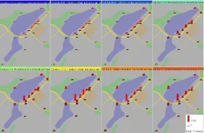
The clusters are represented in a summarized way on a multi-map display as in Figure 3. For the reason of data confidentiality, we do not use a real cartographic background but show the data on top of a schematic drawing. Each of the small maps represents a cluster; the map caption has the colour of the cluster. To obtain a summary of a cluster, the descriptive statistics of the presence values for the places (minimum, maximum, sum, mean, median) are computed from all
situations included in the cluster. One or more of these statistics can be visualized on the multiple maps. In Figure 3, the mean numbers of place visitors are
[image:11.595.126.529.585.694.2]represented on the maps by proportional heights of the bars.
Figure 3. The presence situations are summarized by the clusters. The mean values of the presence are shown by proportional heights of the bars.
same cluster. The multi-map display shows us that the situations are characterized by very high values of presence in the places from which the races are observable and low values in the other places. The differences between the two groups of places are higher on the second day than on the first day, which is explainable by higher interest of the people to the main race than to the qualifying race.
The situations immediately before and after the races were sufficiently similar to be included in the same cluster. They are characterized by high presence of people at the spectator tribunes but also relatively high attendance of the exhibition and shopping places. The situations after the qualifying race on day 1 changed more gradually than after the main race on day 2. By comparing the maps in Figure 3, further observations can be done.
Hence, clustering of presence situations combined with spatial and temporal displays of the clusters allowed us to gain an understanding of the spatio-temporal variation of the people presence.
Analysis of flows
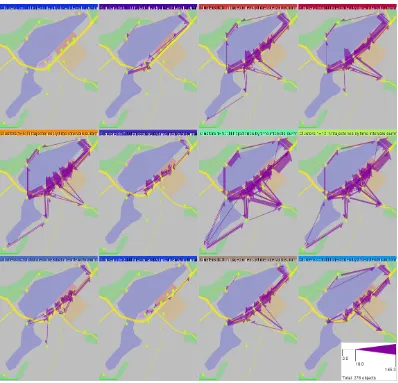
The spatio-temporal variation of the flows is explored analogously to the variation of the presence except that the clustering and visualization tools are applied to the flow situations instead of the presence situations. The flow situation in each time interval is represented by a feature vector consisting of the flow magnitudes (counts of moves and/or moving objects) of the links in this interval. We do the clustering using k-means in the same interactive and iterative way as for the presence. Finally we obtain 12 clusters adequately representing the differences in the flow situations. Figure 4 shows the projection of the cluster centres onto the colour space and the propagation of the cluster colours to the time graph of the counts of moves and to the time mosaic. Figure 5 shows summaries of the clusters on multiple maps where mean flow magnitudes are represented by proportional widths of the flow symbols. Minor flows (with the magnitude below 10) are hidden for reducing the display clutter.
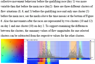
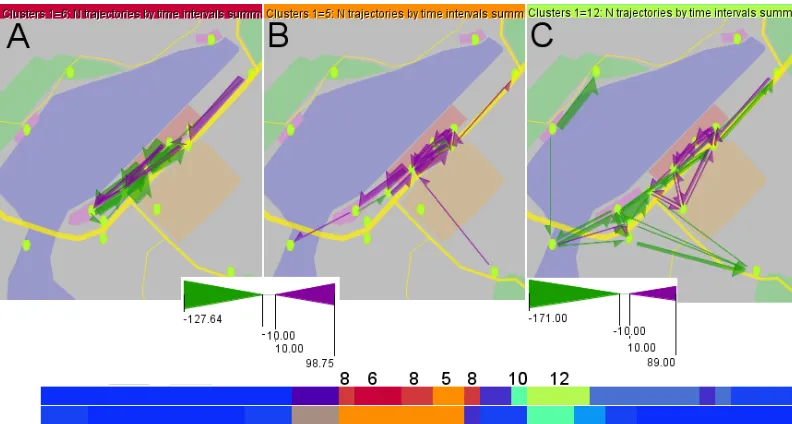
directed towards the tribunes and after the races people mostly moved in the opposite directions. However, there are also some unexpected patterns. The collective movement behaviour before the qualifying race (day 1) was more variable than that before the main race (day2): there are three different clusters of flow situations (8, 6, and 5) before the qualifying race and only one cluster (5) before the main race; see the marks above the time mosaic at the bottom of Figure 6. Also the movements after the races are represented by two clusters (10 and 12) on day 1 and one cluster (10) on day 2. To support examining the differences between the clusters, the summary values of flow magnitudes for one selected clusters can be subtracted from the respective values for the other clusters.
Figure 5. The flow situations have been summarized by the clusters. The mean flow magnitudes are shown.
Figure 6. Differences between temporal clusters of flow situations. A, B: differences in the movements before the races. Clusters 6 (A) and 5 (B) are compared with cluster 8. C: differences in the movements after the races. Cluster 10 is compared with cluster 12. Bottom: the clusters involved in the comparison are marked on a time mosaic display.
Conclusion
The examples show how complex movement data can be analysed by means of visual and computational methods. In fact they demonstrate that collective behaviours of moving objects can be studied and understood by analysing episodic movement data despite the low spatial and temporal coverage and resolution of such data. Aggregation of episodic movement data to some extent compensates for their spatial and temporal sparseness and allows extraction of valuable information about collective movement behaviours of large numbers of moving objects. We argue that this information cannot be extracted by purely computational techniques. Visualisation is essential for enabling human interpretation and involving human knowledge and thinking. However, only visual methods are insufficient due to the large amounts of the data (numerous places, combinatorial number of flows, and long time series), their complexity (the spatial, temporal, and attributive components are hard to visualise together in an easily perceivable way), and massive intersections of the flows in space, which makes them extremely hard to visualise in a comprehensible way. Hence, only a combination of visual and computational methods can turn episodic movement data into knowledge.
We combine visual and interactive techniques with computational clustering of spatial situations emerging due to movements of multiple objects. Spatial displays and interactive operations enable comparison of the space-related properties of the clusters of situations. Temporal displays show the arrangement of the clusters in time and enable perception and investigation of the temporal patterns in the variation of the collective movement behaviour. The methodology is applicable to episodic movement data collected in various ways.
References
Andrienko, G., Andrienko, N., Bak, P., Keim, D., Kisilevich, S., Wrobel, S. A Conceptual Framework and Taxonomy of Techniques for Analyzing Movement. Journal of Visual Languages and Computing, 2011, v.22 (3), pp.213-232
Andrienko, G., Andrienko, N., Bremm, S., Schreck, T., von Landesberger, T., Bak, P., Keim, D. 2010. Space-in-Time and Time-in-Space Self-Organizing Maps for Exploring Spatiotemporal Patterns. Computer Graphics Forum, 29(3), pp. 913-922.
Bak, P., Mansmann, F., Janetzko, H., Keim, D. A. 2009. Spatio-temporal Analysis of Sensor Logs Using Growth-Ring Maps. IEEE Transactions on Visualization and Computer Graphics, 15(6), pp. 913-920.
Boyandin, I., Bertini, E., Lalanne, D. 2010. Visualizing the World’s Refugee Data with JFlowMap. In Poster Abstracts at Eurographics/ IEEE-VGTC Symposium on Visualization. Bruno, R., Delmastro, F. 2003. Design and Analysis of a Bluetooth-based Indoor Localization System. In: Proc. Personal Wireless Communications (PWC), IFIP-TC6 8th International Conference, pp. 711-725.
Guo, D., Chen, J., MacEachren, A., and Liao, K. 2006. A visualization system for space-time and multivariate patterns (VIS-STAMP). IEEE Transactions on Visualization and Computer Graphics, 12(6), pp.1461–1474
Jankowski, P., Andrienko, N., Andrienko, G., Kisilevich, S. 2010. Discovering Landmark Preferences and Movement Patterns from Photo Postings. Transaction in GIS, 2010, v.4 (6), pp.833-852
Keim, D., Andrienko, G., Fekete, J.-D., Görg, C., Kohlhammer, J., Melançon, G. 2008. Visual Analytics: Definition, Process, and Challenges. In: Kerren, A., Stasko, J.T., Fekete, J.-D., North, C. (editors). Information Visualization – Human-Centered Issues and Perspectives. Lecture Notes in Computer Science, Vol. 4950, Springer, Berlin, pp.154-175
Kraak, M.-J., and Ormeling, F. 2003. Cartography: visualization of spatial data. Second edition. Pearson Education Limited, Harlow, UK
Phan, D., Xiao, L., Yeh, R., Hanrahan, P., and Winograd, T. 2005. Flow Map Layout. In Proc. IEEE Symposium on Information Visualization InfoVis 05, Minneapolis, Minnesota, USA, 23-25 October, 2005, pp.219-224
Sammon, J. W. 1969. A nonlinear mapping for data structure analysis. IEEE Transactions on Computers, 18, pp.401–409
Stange, H., Liebig, T., Hecker, D., Andrienko, g., Andrienko, N. 2011. Analytical Workflow of Monitoring Human Mobility in Big Event Settings using Bluetooth. Third International Workshop on Indoor Spatial Awareness ISA 2011, November 1, 2011, Chicago, USA
Vrotsou, K., Andrienko, N., Andrienko, G., Jankowski, P. 2011. Exploring City Structure from Georeferenced Photos Using Graph Centrality Measures. In Proc. Machine Learning and Knowledge Discovery in Databases (PKDD 2011), Lecture Notes in Computer Science, Vol. 6913, pp.654-657
Wood, J., Dykes, J., Slingsby, A. 2010. Visualization of origins, destinations and flows with OD maps. Cartographic Journal, 47(2), pp. 117–129.
Biographies
Natalia Andrienko received her Master degree in Computer Science from Kiev State University in 1985 and PhD equivalent from Moscow State University in 1993. Since 1997, she has been working at GMD, now Fraunhofer IAIS. Since 2007, she is a lead scientist responsible for the visual analytics research. She co-authored the monograph ‘Exploratory Analysis of Spatial and Temporal Data’, over 50 peer-reviewed journal papers, over 20 book chapters and more than 100 conference papers. She received best paper awards at AGILE 2006 and IEEE VAST 2011 conferences, best poster awards at AGILE 2007 and ACM GIS 2011, and VAST challenge award 2008.
Thomas Liebig, research scientist at Fraunhofer IAIS and university of Bonn, was born in 1980 and received his diploma in computer sciences from university of technology, Chemnitz, in 2007. Current research focuses on annual average daily traffic (AADT) estimation, Bluetooth tracking and models for correlations within trajectories.
Hendrik Stange is a project manager at the Knowledge Discovery department of the Fraunhofer IAIS since 2007. He studied Business Information Science specializing on data mining and knowledge management at the Otto-von-Guericke University Magdeburg. His current research interests focus on real-time mobility mining, spatial business intelligence and mobile
communications.
Dirk Hecker is the leader of the Mobility Mining Group at Fraunhofer IAIS. He studied