A method for the evaluation and optimisation of power losses and reliability of supply in a distribution network

A Method for the Evaluation and Optimisation of

Power Losses and Reliability of Supply in a

Distribution Network

J. Ding, K.R.W. Bell, I.M. Elders*

University of Strathclyde Glasgow, UK * [email protected]

Abstract—This paper presents two methods for evaluating and optimizing the configuration of a distribution network. A new loss-optimization method is described which partitions, optimizes and then recombines the network topology to identify the lowest loss configurations available. A reliability evaluation method is presented which evaluates, on a load-by-load basis, the most effective restoration path and the associated time. In contrast to previously-reported methods, the operation of different types of switch is integrated into this approach, reducing dependency on pre-determined restoration times for each load each fault location. This provides a more accurate estimate of the outage durations through identification of the specific restoration method for each load under each fault condition. The optimization method applied is shown to be effective in identifying optimally-reliable network topologies. Significant benefits are shown to be available.

Index Terms—Optimization; Power System Planning; Power System Reliability.

I. INTRODUCTION

Minimization of energy losses and maximization of the reliability of supply to customers are among the principal objectives of electricity distribution network operators (DNOs), and also form important metrics of network performance. As such, they are also of interest to regulators, governments and other stakeholders. Comparison of these metrics between DNOs is an important theme of regulatory performance assessment.

The particular operational configuration of the distribution network – that is, the configuration of open and closed switches which govern the routes by which current flows from source to customer – is an important determinant of network losses and supply reliability. However, a configuration which is optimal from the perspective of losses may not offer the best security of supply and vice versa. Furthermore, other constraints on network configuration must be considered, such as thermal limits on branch current or the capabilities of the protection system which often require a radial configuration.

Changes in the location and nature of load, and the development of small-scale generation such as solar PV may alter the distribution of losses, while network reinforcement or investment in improved protection and distribution automation can offer opportunities to improve supply reliability metrics if appropriately located and configured.

It is clear therefore that DNOs will be expected to show that they are taking these two factors into account in the future design and operation of their networks, and that tangible benefits to customers are being produced. However, optimization of both losses and supply reliability is a complex task and as previously noted, it will often be necessary to trade off one against the other to identify the position of most benefit. In this paper, we present methods for both the optimization of distribution network losses by feeder reconfiguration, and for evaluation and optimization of supply reliability.

Section II briefly reviews methods of loss minimization and of analysis and optimization of reliability. In section III we describe a new method of loss minimization in which the network is partitioned to find a global optimum configuration at acceptable computational cost. Section IV describes a method for evaluating network reliability metrics taking into account the actual restoration methods that would be applied in the case of different potential faults. Section V applies this method together with an optimization approach similar to that used for losses to identify an optimally reliable network configuration.

II. BACKGROUND

A. Loss Minimization

Network losses can be minimized by reconfiguration of the power system to achieve a more favorable distribution of current among the branches of the network. Loss reduction by phase balancing can also be achieved, but is likely to be more costly and intrusive in comparison to reconfiguration through the movement of open points.

Three main approaches to reconfiguration planning for loss minimization have been reported, namely heuristic approaches, biologically-inspired methods and deterministic methods.

Heuristic approaches apply guided search techniques and ‘rules of thumb’ to generate an approximation to a lowest loss configuration for the power network. Shirmohammadi and Huang [1] reported a method for de novo identification of open points within a network based on an analysis of current circulation in loops in the network. This method was refined by Goswani and Basu [2] to reconsider open points individually starting from an initial network configuration. Raju and Bijwe [3] apply a branch exchange method considering active power sensitivity and branch impedances. An important disadvantage of heuristic methods is that they may not identify the global optimum configuration, particularly in complex networks with many inter-related configuration options. Also, [4] shows the importance of using heuristics appropriate to the behavior of the network, for example, in the relationship between the voltage profile and changes in losses resulting from reconfiguration.

A number of biologically-inspired approaches have been reported, of which the Genetic Algorithm (GA) appears the most commonly used, although Particle Swarm Optimization (PSO) has attracted interest more recently [5]. Reconfiguration problems are well-suited to such methods, though in large or complex networks the model of the network configuration may be cumbersome, and the search space sparse: many potential configurations will not meet electrical or topology constraints. Mendoza et al [6] showed that generating an initial population of radial candidate configurations can improve performance here. The risk of finding a local rather than global optimum must also be considered along with the frequency with which a network could or should be reconfigured compared with the solution time of the algorithm being used.

Deterministic approaches generally involve reformulation of the power network into a mathematical model which is then optimized by methods such as linear programming. Ramos et al [7] reported an approach based on a “path to node” concept, which was subsequently improved by Khodr et al [8] using an improved network loss model. More recently, Ahmadi and Marti [9] reported a Mixed Integer Quadratic Programming approach based on a simplified load model. Inoue et al [10] apply a search-based approach using the Binary Decision Diagram, partitioning of complex networks, and a simplified power flow model based on current addition. The approximations necessary to construct a tractable mathematical model of network losses for such methods may detract from their ability to identify the global optimum.

B. Reliability Evaluation and Optimization

Under the regulatory regime applicable to DNOs in Great Britain (GB), the principal reliability metrics in use, and which form the basis of an incentive and penalty scheme [11], are average Customer Interruptions per hundred customers (CI) and average Customer Minutes Lost (CML), defined as:

 _



f CI

C

i i

 

 C

T f CML

C

i i i





 1

 

In (1) and (2), C is the total number of customers of the DNO, fi is the number of fault outages experienced by customer

i, and Ti is the average interruption duration experienced by

customer i. It should be noted at “short interruptions” of less than three minutes duration are excluded from this calculation. A number of methods have been reported for the evaluation of network reliability metrics. Monte Carlo simulation approaches have been widely used, particularly in relation to transmission and generation-related problems [12]. Markov model-based approaches [13] and direct analytical approaches are also reported. Some previous work has considered the involvement of protection [14] and automation systems [15, 16]. These considerations are particularly important in distribution networks since an important driver of investment in improved protection and distribution automation is the improvement of service to customers that they make possible, not least in respect of service restoration time. Nevertheless, manually controlled and especially manually-undertaken switching remain important determinants of the supply restoration time which is experienced by most customers.

Accurate evaluation of the optimal restoration path, considering actual switching times as well as automation capabilities and repair times, is vital to the calculation of precise reliability metrics and thus to the selection of the optimal configuration for reliability. This issue is not fully addressed in the literature and is thus considered in this paper.

III. LOSS OPTIMIZATION

The loss optimization method presented in this paper considers a distribution network subject to a radial configuration constraint, which is to say that the network is without islands, and also without loops in the topology – all loads are thereby connected to exactly one grid infeed. The problem is further constrained by power flow and voltage limits. While this significantly reduces the solution space, for moderately large or complex networks, the number of valid topologies is still prohibitively large for practical loss evaluation and optimization. We therefore partition the network into sub-networks or “zones” of tractable complexity which are then optimized individually.

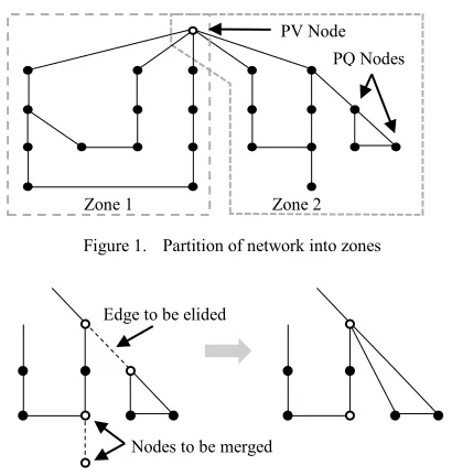
The network is initially represented as an undirected potentially-cyclic graph, composed of nodes connected by edges in the conventional fashion. Nodes are categorized as “PV” nodes (having a source of infeed with controllable voltage magnitude) and “PQ” nodes in the usual way. “PV edges” are defined as those edges which are immediately adjacent to a PV node. Beginning at a root infeed node, a breadth first search is used to assign a “layer number” to each node; this is then used to convert the undirected graph into a directed graph in increasing order of layer number, as shown in Fig. 1 in which edges are uniformly directed downwards.

the corresponding PV node to identify all PQ nodes which may be reached without passing through another PV edge. These nodes, together with the PV nodes adjacent to the initiating and terminating PV edges, are defined as forming a zone. The process is shown in Fig. 1.

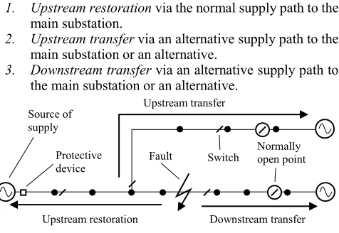
Zonal graphs are simplified by eliding topologically redundant edges which must remain closed in order to satisfy the constraint that all nodes must be connected to a PV node, and by merging their adjacent PQ nodes, as shown in Fig. 2. The zone is now represented by a graph which is often but not necessarily cyclic.

All possible spanning trees of this graph are now generated by a recursive algorithm [17]. The spanning trees each represent a potential topology of the zone which is radial and in which all loads are supplied.

Figure 1. Partition of network into zones

Figure 2. Elision of topologically redundant edges and merger of nodes

Each topology for each zone is then evaluated, with elided edges and nodes restored, using Newton-Raphson power flow analysis to determine losses. Topologies for which convergence is not obtained are considered infeasible and are discarded. Typically this has been found to occur because of significant violation of branch thermal constraints or long supply paths leading to voltage drop. The result of this step is a ranked list of feasible topologies for each zone in order of loss-optimality.

The zone topologies are then re-assembled into a complete network topology by separating any previously merged PV nodes and combining the highest ranked topology for each zone. This avoids the combinatorial explosion which would result from exhaustive combination of zone topologies, but may introduce inaccuracy in the identification of the global optimum, since the overall loss of the combined network may differ from the aggregate loss of its component zones. Inoue et al [10] report that their similar partitioning approach produces effective results. Nevertheless, to increase confidence in selection of the optimum configuration, a small set of alternative network topologies is constructed by using second ranked topologies for certain zones which are close in

performance to the highest ranked topology for the zone. Losses in each of these complete topologies are then evaluated using power flow analysis to identify the optimum configuration.

IV. RELIABILITY EVALUATION

The objective of the reliability evaluation algorithm described in this paper is to evaluate the CI and CML reliability metrics defined in section II above. The method considers single independent fault events: multiple simultaneous or overlapping fault events are not considered, although the method could be extended to do so.

To evaluate the reliability metrics, information about the network topology is required, in the form of an undirected graph similar to that outlined in section III, and in which protection devices, remote-control switches and manual switches are identified. Switching times for these devices are required, as well as (for non-reclosable devices such as fuses) repair times. The number of customers supplied from each node is also required, as are the failure rate and repair rate for each branch. Generic failure and repair rates for branch types (e.g. overhead lines, underground cables at particular voltages), together with section lengths may be used where specific rates are not known.

The reliability evaluation proceeds in three main stages: 1. Navigation and pre-processing of the network

topology.

2. Evaluation of effects of each potential fault. 3. Calculation of reliability metrics.

A. Network Navigation and Preprocessing

The objective of this step is to convert the initially undirected graph, in which normally-open points are defined to meet the constraint of a radial configuration into a directed graph which is partitioned into individual feeders radiating from the main substation. In addition, the zone of protection of each protective device is identified. This is achieved by means of a breadth-first search beginning at a protective device adjacent to the root node and terminating at protective devices or normally open points – this defines the zone of protection of the initial device. The process is repeated beginning from either a terminating protective device or one adjacent to the root node until all nodes have been searched.

As a result of this preprocessing step, all network branches have an assigned ‘upstream’ and ‘downstream’ direction, and a set of branches Pp is defined as the zone of protection for each

protective device p – that is to say the set of faults to which device p would respond.

B. Fault Effect Evaluation

The fault effect evaluation step is carried out for each potentially faulted branch bi in the network, and involves the

identification of nodes affected by the fault, the determination of the restoration method to be applied to each node and the calculation of the restoration time for each node.

To identify the set Fi of affected nodes, the zone of

protection Pp containing bi is identified. The downstream nodes

of all members of Ppare members of Fi. The network graph is

then traversed downstream from bi to normally open points. The

downstream nodes of the members of each protection zone

Zone 2 Zone 1

PV Node PQ Nodes

Edge to be elided

encountered during this traversal are added to Fi. At the

conclusion of the traversal, set Fi contains all nodes which will

experience interruption as a result of a fault on bi.

To determine the restoration method and time to be applied to each node nj in Fi, a number of time metrics are defined:

tpr Time to reset and reclose a protective device

trc Switching time for a remote-control switch

tm Switching time for a manual switch

tnop Switching time for a normally-open point

tr Repair time for fault on bi

tres,XY Restoration time for nodes between points X and Y

It is assumed that trc < tm and that switching actions are

undertaken sequentially. Although uniform values of these time metrics are used here, it will be appreciated that specific values could be used for individual switches and protective devices where these are known.

Three restoration methods are considered, in the following order, and are illustrated in Fig. 3:

1. Upstream restoration via the normal supply path to the main substation.

2. Upstream transfer via an alternative supply path to the main substation or an alternative.

3. Downstream transfer via an alternative supply path to the main substation or an alternative.

Figure 3. Available restoration methods

Upstream restoration is considered first. The network is traced from the fault F to the nearest upstream protective device P to the fault, noting the first-encountered remote-control switch R and the first encountered manual switch M, forming the restoration path. It should be noted that either R, M or both may be absent. The sequence of restoration actions is dependent on the sequence of P, R, M and F:

 P-R-M-F: The first restoration step is to open R and then close P, restoring nodes between those points, as shown in (3). The second restoration step is to open M and reclose R as in (4). Nodes downstream of M cannot be restored by switching and are restored in repair time as shown in (5):

 tres,PR = tpr + trc 

 tres,RM = tpr + 2trc+ tm 

tres,MF = tr (5)

 P-R-F or P-M-R-F: The first restoration step is to open R and close P. Nodes downstream of R cannot be restored by switching. It will be noted that M does not contribute to supply restoration:

tres,PR = tpr + trc (6)

tres,RF = tr (7)

 P-M-F: The first restoration step is to open M and close P. Remaining nodes are subsequently restored on fault repair.

tres,PM = tpr + tm (8)

tres,MF = tr (9)

 P-F: No switches are available to expedite supply restoration. All nodes are restored on fault repair.

tres,PF = tr (10)

Upstream transfer is a potential supply restoration approach where an alternative supply route exists from a normally open point to the upstream restoration path, as shown in Fig. 3. The network is traced upstream from each normally open point to either an intersection with the upstream restoration path or a source of supply. Where the upstream restoration path is intersected, the search identifies the normally open point O; the point of intersection I and its corresponding restoration time tres,I

by upstream restoration; the remotely controlled switch R nearest to I and the manually controlled switch M nearest to I. As for upstream restoration, the order of O, R, M and I governs the restoration time for nodes between O and I:

 O-R-M-I: Transfer nodes between O and R, then between R and M. Remaining nodes are restored in repair time.

tres,OR = min(tnop + trc ,tres,Inr) (11)

tres,RM = min(tnop + 2trc + tm ,tres,I) (12)

tres,MI = tres,I (13)

 O-R-I or O-M-R-I: Transfer nodes between O and R, and restore remaining nodes on fault repair.

tres,OR = min(tnop + trc ,tres,I) (14)

tres,RI = tres,I (15)

 O-M-I: Transfer nodes between O and M. tres,OM = min(tnop + tm ,tres,I) (15)

tres,MI = tres,I (16)

Where there is no switch between O and I, restoration by upstream transfer is not possible:

Fault Protective

device

Upstream transfer Source of

supply

Normally open point Switch

tres,OI = tres,I (17)

Downstream transfer is possible where a normally open point exists downstream of the fault. The network is traced downstream from the fault F to the normally open point O, noting the nearest remote-controlled switch R and manual switch M to the fault. Restoration times are once again dependent on the order of O, R, M and F and are as shown for the upstream transfer case, but with F substituted for I.

The result of the fault effect evaluation is that the interruption duration ti,j for each node nj affected by a fault on

each branch bi is known. This is particularly important in the

calculation of reliability metrics (such as those applicable in GB) in which the relationship of interruption duration to a threshold is considered.

C. Reliability Metric Calculation

The calculated interruption durations are now used, together with equipment fault rates and customer numbers to calculate the network reliability metrics. Point indices are calculated first for each node nj:

 





min 3 ,i,j i

j Ft

n

i

j





 

 







min 3 ,

,

,j i i j Ft

n

j i i

j

t

T



 

where λi is the fault rate for branch bi, λj is the interruption rate

for node nj, Tj is the average annual interruption duration for

node nj and other symbols have the previously assigned

meanings. It should be noted that, as a consequence of the GB regulatory arrangements mentioned in section II, interruptions that are shorter than three minutes are excluded from these metrics. System indices can then be calculated:



100

 





 

N n

j N n j j

j j

C C CI



 







 



N n

j N n

j j

j j

C C T CML

 

where N is the set of all nodes in the network and Cj is the

number of customers supplied from node nj.

This method improves the accuracy of the calculated reliability metrics, since they are reflective of the precise method which will be used to restore each individual load.

V. RELIABILITY OPTIMIZATION

The reliability optimization is achieved using a similar approach to that of the loss optimization method described previously. However, whereas in that case the objective was to

minimize the active power loss in the network, reliability optimization presents three possible objectives, namely the maximization of regulatory reward in relation to either CI or CML, or the optimization of the combined regulatory reward under those two metrics. A regulatory penalty is considered as a negative reward. The regulatory reward is used as a mechanism to compare the relative weight of the two quantities. An objective function F(T) can be defined for each of these objectives in which a trial network configuration T is compared to a reference configuration R:



F

(

T

)





CI



CI





I



F

(

T

)





CML



CML





I



F

(

T

)



F

(

T

)



F

(

T

)

where CIC is the CI metric for configuration C, CMLC is the

CML metric for configuration C and IM is the reward or penalty

rate (in £/CI or £/CML) for metric M. In the GB incentive scheme mentioned above, these rates are set by the regulator and are specific to each DNO.

The method of reliability optimization proceeds as previously. First, the network is partitioned into zones and simplified according to the relationships between PQ nodes and sources of supply. The positions of normally open points within these zones are optimized considering their spanning trees. As before, a power flow analysis is carried out of each candidate zone configuration, although in this case it is solely to validate the feasibility of the configuration in relation to voltage and thermal constraints. Feasible zone configurations are then evaluated using the method described in section IV to determine their CI and/or CML metrics, and (22), (23) or (24) applied to evaluate the appropriate objective function.

Feasible configurations for each zone are ranked by objective function. As for loss optimization, combinations of the two highest ranked candidate configurations for each zone are constructed as candidate complete network configurations. The feasibility of these candidates is once again checked by power flow analysis, and the appropriate reliability metric and objective function calculated for the complete network is calculated in order to promote selection of the globally optimum network configuration.

It will be observed that the reliability optimization process exhibits considerable commonality with the loss optimization method, and that savings in time and computation may be achieved by conducting them as a single process to the point at which candidate zone configurations are ranked according to the quantity to be optimized.

evaluated according to the combined metric. Repeating the process with zonal ranking according to the reliability metric shows the effects of the incentive weights on the overall optimization results.

VI. CASE STUDIES

A. Loss Optimization

Fig. 4 shows a typical section of GB urban distribution network, adapted from part of the ScottishPower Manweb 11kV network [18]. It has four sources of supply, in the form of 33/11kV ‘primary’ substations, 221 branches and 195 nodes, of which 191 supply customer loads. Twenty-five 11kV feeders (corresponding to PV edges) lead away from the primary substations. Fifteen normally open points must be placed within the network to meet the requirement for a radial configuration. In the initial configuration shown, the total loss is 0.760MW.

Figure 4. Typical GB 11kV distribution network

The partitioning method described in section III above divides the network into ten zones, as shown in Table I.

TABLE I. PARTITION OF 11KV NETWORK INTO ZONES

Zone Possible

topologies

Feeders Branches Nodes

1 4 2 6 7

2 788 4 29 29

3 9 2 11 12

4 10 2 12 13

5 5 2 7 8

6 7 2 9 10

7 7 2 36 37

8 8 2 10 11

9 14 5 17 18

10 12219 5 84 82

It can be seen that zone 10 exhibits considerably more complexity in comparison to the others, most of which are simple loops with little interconnection between feeders.

After optimization of the zonal topologies, ten complete network topologies are constructed from top and second-ranked zone configurations. Of the required fifteen normally open points, ten are common to all ten candidate topologies. Ten further normally open points appear in the ten topologies. Four of the original normally open points appear in

one or more of the ten candidate topologies. This indicates that the well-performing topologies tend to be mutually similar in this case, but are much less similar to the initial topology.

Active power losses, in increasing order, are shown in Table II. The losses of the whole network configurations are found to be in the region of 0.5% larger (in this case, approximately 2.5 – 3kW) than the sum of their constituent zonal topology losses when calculated individually.

TABLE II. ACTIVE POWER LOSSES OF CANDIDATE TOPOLOGIES

Topology Losses

(MW)

Topology Losses

(MW)

1 0.4830 6 0.4832

2 0.4830 7 0.4832

3 0.4831 8 0.4832

4 0.4831 9 0.4833

5 0.4832 10 0.4833

It can be seen that the ten generated candidate topologies are very similar in terms of losses, indicating that the selection of first and second-ranked zonal topologies is successful in identifying near-optimal complete network topologies. It appears unlikely that evaluation of a larger set of complete network topologies, or use of lower-ranked zonal topologies would result in the identification of a lower-loss network configuration. The significant improvement over the initial configuration is reflective of the lack of similarity of the optimal and near-optimal topologies to it.

B. Reliability Optimization

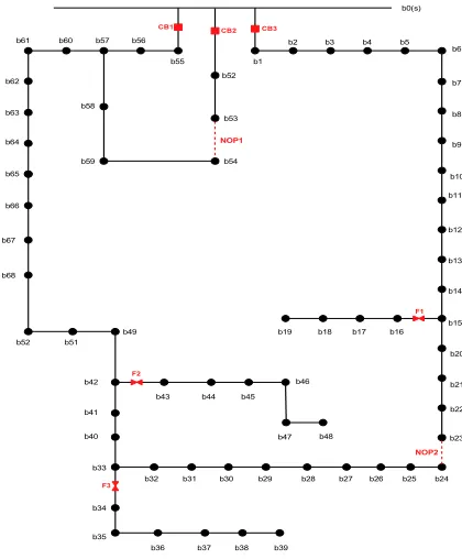
Fig. 5 shows a portion of a typical GB urban 11kV network supplied from a single 33/11kV substation (again adapted from ScottishPower Manweb data [18]). For clarity of exposition, this is smaller in scope than that of Fig. 4.

Figure 5. Portion of GB 11kV distribution network

b1

b2 b3 b4 b5 b6 b7 b8 b9 b10 b11 b12 b13 b14 b15 b16 b17 b18 b19

b20 b21 b22 b23 b24 b25 b26 b27 b28 b29 b30 b31 b32 b33

b55 b56 b57 b60 b61 b62 b63 b64 b65

b40 b41 b42

b49 b51 b52 b66 b67 b68

b34 b35

b36 b37 b38 b39 b43 b44 b45

b46

b47 b48 b52

b53 b54 b59

b58

NOP1

NOP2 b0(s) CB1 CB2 CB3

F1

F2

There are 69 nodes and 70 branches, each of which can be individually manually switched with a switching time of two hours. The three feeders are protected by circuit breakers whose switching time is negligible, and three spurs are protected by fuses with a negligible switching time and a repair time of 1.1 hours. Two normally open points are required for a radial configuration. Three remotely-controlled switches, with a switching time of one minute are placed a quarter, a half and three-quarters of the way around the large loop shown in Fig. 5. Reward rates are set at £70,000 per unit for CI and £210,000 per unit for CML, applicable under the GB Interruption Incentive Scheme [19]. The calculated reliability statistics for the initial configuration shown are 28.153 interruptions per hundred customers per year and 17.156 minutes per customer per year, which are taken as the base values CIR and CMLRfor

the calculation of the objective function FCI+CML(T).

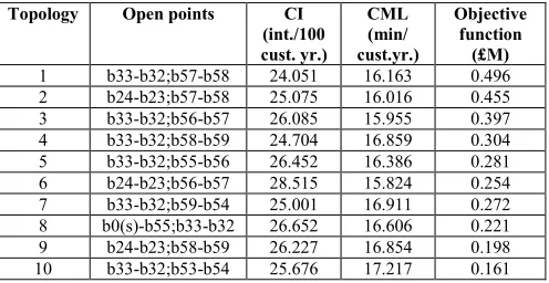
In order to select the optimal locations of normally open points to maximize the reliability metric, the network is partitioned into zones, and the reliability of the topologies of each is calculated and ranked. Ten complete network topologies are constructed from the highest-ranked zonal topologies, as shown in Table III:

TABLE III. RESULTS OF RELIABILITY OPTIMIZATION OF TOPOLOGY

Topology Open points CI

(int./100 cust. yr.)

CML (min/ cust.yr.)

Objective function

(£M)

1 b33-b32;b57-b58 24.051 16.163 0.496

2 b24-b23;b57-b58 25.075 16.016 0.455

3 b33-b32;b56-b57 26.085 15.955 0.397

4 b33-b32;b58-b59 24.704 16.859 0.304

5 b33-b32;b55-b56 26.452 16.386 0.281

6 b24-b23;b56-b57 28.515 15.824 0.254

7 b33-b32;b59-b54 25.001 16.911 0.272

8 b0(s)-b55;b33-b32 26.652 16.606 0.221

9 b24-b23;b58-b59 26.227 16.854 0.198

10 b33-b32;b53-b54 25.676 17.217 0.161

In comparison to the base case, significant reliability benefits can be gained through topology optimization. The range of performance is much wider than was observed for loss optimization, although this is partly reflective of the smaller and simpler network. CI is reduced by almost 15%, and CML by almost 6%, representing an improvement in the reliability of supply experienced by customers. It is clear that both reliability metrics must be considered: although the optimal configuration has the best CI value, its CML value is not the lowest identified, and neither metric reduces monotonically as the combined metric improves.

Distinct patterns are noticeable in the placement of the normally open points in these high-ranking topologies. One is usually placed either at the existing location at the bottom right of the diagram or close to the lowest spur, with the other either on the left of the upper loop in the diagram, or in the section of network common to the two loops. In this latter case, the objective function appears quite sensitive to the location of the normally open point, suggesting that regular review of its position by the DNO in response to any change in input conditions (such as customer numbers) may be advisable.

A joint optimization of losses and reliability for the network shown in Fig. 5 has also been carried out. This showed that reliability incentives tended to dominate unless very high loss costs were applied. The overall result was therefore to prefer the optimally reliable configuration.

VII. CONCLUSIONS AND FURTHER WORK

A potential deficiency of existing distribution network loss optimization methods is that, in reducing the representation of the network to a tractable form, or in applying heuristics to transform the network into a lower-loss configuration, approximations and inaccuracies may be introduced which risk a failure to identify the globally optimal network configuration. In this paper, we have shown that partition of the network into smaller, topologically simplified units, which can be exhaustively evaluated to identify their loss-optimal configuration is effective in addressing this problem. This result is achieved since the assembly of lowest and near-lowest-loss configurations of these units into complete network topologies produces a set of similarly-performing low-loss candidates for an optimal network configuration.

Previously reported methods to evaluate and optimize the reliability of distribution networks do not consider the precise method, including manual switching, used to restore supply to customers. The method introduced here incorporates such switching into an overall restoration plan for each load including automated and remotely-controlled devices, ensuring accuracy in the reliability metrics calculated. We have also shown that the application of a similar process of partitioning, optimizing and recombining as is applied to losses can produce significant benefits through identifying an optimally reliable network configuration and improving service to customers.

The effect of distributed energy resources (which may allow otherwise infeasible restoration methods) on the calculation and optimization of reliability is not yet considered by the method described here, and forms a topic for future research. Other topics for further investigation include a more precise evaluation of switching sequences to achieve a changed configuration while not interrupting any supply in the meantime or risking inadvertent operation of protection; extension of the methods to networks in which the approach to protection permits operation with closed loops (and to show the potential benefits of such an approach); and an evaluation of network reconfiguration through a typical year of operation given time series profiles of demand and generation. This would allow annual losses to be quantified and an assessment of how often a network should be reconfigured to be in its optimal state and what this means for the burden placed on control room staff and the need for automation. Finally, the methods will be incorporated within design tools allowing network planners to evaluate the best locations for new switches with remote control and perform the associated cost-benefit analysis.

REFERENCES

[1] D. Shirmohammadi and H. W. Hong, "Reconfiguration of electric distribution networks for resistive line losses reduction," IEEE Trans.

Power Delivery, vol. 4, pp. 1492-1498, 1989.

[2] S. K. Goswami and S. K. Basu, "A new algorithm for the reconfiguration of distribution feeders for loss minimization," IEEE Trans. Power

[3] G. Raju and P. R. Bijwe, "An efficient algorithm for minimum loss reconfiguration of distribution system based on sensitivity and heuristics," IEEE Trans. Power Systems, vol. 23, pp. 1280-1287, 2008. [4] M. E. Baran and F. F. Wu, "Network reconfiguration in distribution

systems for loss reduction and load balancing," IEEE Trans. Power

Delivery, vol. 4, pp. 1401-1407, 1989.

[5] A.Y. Abdelaziz et al, “A modified particle swarm algorithm for distribution systems reconfiguration,” presented atIEEE PES General

Meeting, Calgary, AB, July 2009.

[6] J. Mendoza et al, "Minimal loss reconfiguration using genetic algorithms with restricted population and addressed operators: real application,"

IEEE Trans. Power Systems, vol. 21, pp. 948-954, 2006.

[7] E. R. Ramos, A. G. Exposito, J. R. Santos, and F. L. Iborra, "Path-based distribution network modeling: application to reconfiguration for loss reduction," IEEE Trans. Power Systems, vol. 20, pp. 556-564, 2005. [8] H. M. Khodr, J. Martinez-Crespo, M. A. Matos, and J. Pereira,

"Distribution systems reconfiguration based on OPF using Benders Decomposition," IEEE Trans. Power Delivery, vol. 24, pp. 2166-2176, 2009.

[9] H. Ahmadi and J.R. Marti, “Linear current flow equations with application to distribution systems reconfiguration,” IEEE Trans Power

Systems, vol. 30, pp. 2073-2080, 2014.

[10] T. Inoue et al, “Distribution loss minimization with guaranteed error bound,” IEEE Trans. Smart Grid, vol. 5, pp. 102-111, 2014.

[11] Office of Gas and Electricity Markets, “Information and incentives project incentive schemes: final proposals,” Ofgem, London, Dec. 2001.

[12] A. M. Rei and M. T. Schilling, "Reliability assessment of the Brazilian power system using enumeration and Monte Carlo," IEEE Trans. Power

Systems, vol. 23, pp. 1480-1487, 2008.

[13] R. E. Brown, S. Gupta, R. D. Christie, S. S. Venkata, and R. Fletcher, "Distribution system reliability assessment using hierarchical Markov modeling," IEEE Trans. Power Delivery, vol. 11, pp. 1929-1934, 1996. [14] J. J. Meeuwsen, W. L. Kling, and W. A. G. A. Ploem, "The influence of protection system failures and preventive maintenance on protection systems in distribution systems," IEEE Trans. Power Delivery, vol. 12, pp. 125-133, 1997.

[15] Y. He, L. Soder, and R. N. Allan, "Evaluating the effect of protection system on reliability of automated distribution system," presented at the

Power Systems Computation Conference (PSCC), Seville, Spain, 2002.

[16] D. Fahmi, et al, “Evaluation of distribution network reliability index using loop restoration scheme”, presented at 1st _{International} Conference on Information Technology, Computer and Electrical

Engineering, Semarang, 2014.

[17] H. N. Gabow and E. W. Myers, "Finding all spanning trees of directed and undirected graphs," SIAM J. Comput., vol. 7, pp. 280-287, 1978. [18] SP Energy Networks, “SP Manweb Long Term Development

Statement”. [Online]. Available: http://www.spenergynetworks.co.uk/ pages/long_term_development_statement.asp