Numer. Math.
DOI 10.1007/s00211-016-0822-1
Numerische
Mathematik
Local two-sided bounds for eigenvalues of self-adjoint
operators
G. R. Barrenechea1 · L. Boulton2 · N. Boussaïd3
Received: 20 January 2015 / Revised: 27 April 2016
© The Author(s) 2016. This article is published with open access at Springerlink.com
Abstract We examine the equivalence between an extension of the Lehmann– Maehly–Goerisch method developed a few years ago by Zimmermann and Mertins, and a geometrically motivated method developed more recently by Davies and Plum. We establish a general framework which allows sharpening various previously known results in these two settings and determine explicit convergence estimates for both methods. We demonstrate the applicability of the method of Zimmermann and Mertins by means of numerical tests on the resonant cavity problem.
Mathematics Subject Classification 65M60·65L60·65L15·65N12
1 Introduction
In this work we study in close detail the equivalence between two pollution-free techniques for numerical computation of eigenvalue bounds for general self-adjoint
B
G. R. Barrenechea[email protected] L. Boulton
[email protected] N. Boussaïd
1 Department of Mathematics and Statistics, University of Strathclyde, 26 Richmond Street, Glasgow G1 1XH, Scotland
2 Department of Mathematics and Maxwell Institute for Mathematical Sciences, Heriot-Watt University, Edinburgh EH14 4AS, UK
operators: a method considered a few years ago by Zimmermann and Mertins [35], and a method developed more recently by Davies and Plum [23]. These two methods are pollution-free by construction and have been proven to provide reliable numerical approximations.
The approach of Zimmermann and Mertins is built on an extension of the Lehmann– Maehly–Goerisch method [4,26,33] and it has proven to be highly successful in various concrete applications. These include the computation of bounds for eigenvalues of the radially reduced magnetohydrodynamics operator [15,35], the study of complemen-tary eigenvalue bounds for the Helmholtz equation [6] and the calculation of sloshing frequencies [4,5].
The method of Davies and Plum on the other hand, is based on a notion of approxi-mated spectral distance and is highly geometrical in character. Its original formulation dates back to [21–23] but it is yet to be tested properly on models of dimension larger than one.
In this work we follow the analysis conducted in [23, Section 6] where the equiv-alence of both these techniques was formulated in a precise manner. Our main goal is two-fold. On the one hand we examine more closely the nature of this equivalence by considering multiple eigenvalues. On the other hand we determine sharp estimates for both methods. These results include convergence and error estimates for both the eigenvalues and associated eigenfunctions. We finally illustrate the applicability of the method of Zimmermann and Mertins using the Maxwell eigenvalue problem as benchmark.
1.1 Context, scope and contribution of the present work
The computational approach considered in this work has a “local” character, in the sense that a shift parameter should be set before hand. The methods derived from this approach only provide information about the spectrum in a vicinity of this parameter, in similar fashion as the Galerkin method gives information only about the eigenvalues below the bottom of the essential spectrum. They give upper bounds for the eigenvalues to the right of the parameter and lower bounds for the eigenvalues to the left of it.
The method of Davies and Plum primarily relies on the geometrical properties of a notion of approximated spectral distance. We introduce this notion in Sect.3. Our Proposition2was first formulated in [21, theorems 3 and 4]. These statements played a fundamental role in the proof of [23, Theorem 11] which provided crucial connections with the method of Zimmermann and Mertins. In Proposition5and Corollary6we establish an extension of [21, theorems 3 and 4] allowing multiple eigenvalues. These rely on convexity results due to Danskin (see Lemma4and [8, Theorem D1]) and they are of fundamental importance in various parts of our analysis.
Theorems13and14, and Corollary15, are precise formulations of convergence in the setting of the method of Davies and Plum. The two theorems differ from one another in that a higher order of approximation occurs when the shift parameter is away from the spectrum. In Theorem16we show that, remarkably, the method of Zimmermann and Mertins always renders the higher order of approximation as a consequence of Corollary15. This is, for instance, in great agreement with the results presented in [34], which compare the errors in Lehmann–Goerisch and Rayleigh–Ritz bounds (see also [28], where convergence of iterative solvers is studied).
In Proposition7we establish upper bounds for error estimates for eigenfunctions in terms of spectral gaps. This statement is related to similar results of Weinberger [32] and Trefftz [30]. See also [33, Chapter 5]. The precise connection between Proposi-tion7and all these results is unclear at present and will be examined elsewhere.
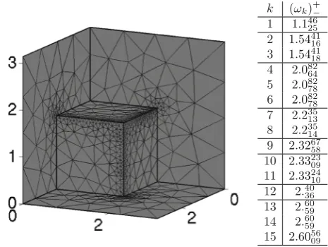
The model of the isotropic resonant cavity that we consider in Sect.6has been well-documented to render spectral pollution when the classical Galerkin method and finite elements of nodal type are employed for numerical approximation. We show by means of numerical tests that, remarkably, the method of Zimmermann and Mertins provides robust and accurate approximations of the eigenvalues of the Maxwell operator even when implemented on standard Lagrange elements. By construction, this method is free from spectral pollution. A more systematic investigation in this respect with many more numerical tests (including anisotropic media), a convergent algorithm and a reference to a fully reproducible computer code can be found in [3].
Preliminary information on the number of eigenvalues in a given interval, which might or might not be available in practice, allows the determination of enclosures from the one-sided bounds produced by the approaches discussed in this work. Convergence also yields enclosures in suitable asymptotic regimes. The algorithm described in [3] is an example of a concrete realisation of this assertion.
1.2 Outline of the analysis
Section2 includes the notational conventions and assumptions which will be used throughout this work. Section3sets the general framework of approximated spec-tral distances and their geometrical properties. There we also discuss approximation of eigenspaces with explicit estimates. The method of Zimmermann and Mertins is derived in Sect.4and its convergence is established in Sect.5. These two sections comprise the main contribution of this work. The final Sect.6is devoted to illustrating a concrete computational application of the method of Zimmermann and Mertins to the resonant cavity problem.
2 Preliminary notation, conventions, and assumptions
LetA:D(A)−→Hbe a self-adjoint operator acting on a Hilbert spaceH. Decom-pose the spectrum of A in the usual fashion, as the disjoint union of discrete and essential spectra, σ (A) = σdisc(A)∪σess(A). Let J be any Borel subset of R. Below the spectral projector associated to Ais denoted by1J(A)=
JdEλ, so that
Eλ(A)=E{λ}(A). GenerallyEJ(A)⊆1J(A)H, however there is no reason for these
two subspaces to be equal except when the spectrum withinJ is only pure point. Everywhere belowt∈Rwill denote a scalar parameter. This is the shift parameter which is intrinsic to the methods.
Letlt :D(A)×D(A)−→Cbe the (not necessarily closed) bi-linear form
associ-ated to(A−t),
lt(u, w)= (A−t)u, w ∀u, w∈D(A).
Letqt :D(A)×D(A)−→Cbe the closed bi-linear form
qt(u, w)= (A−t)u, (A−t)w ∀u, w∈D(A). (1)
For anyu ∈ D(A)we will constantly refer to the followingt-dependant semi-norm, which is a norm iftis not an eigenvalue,
|u|t =qt(u,u)1/2= (A−t)u. (2)
By virtue of the min–max principle,qt characterises the part of the spectrum of the
positive operator(A−t)2which lies near the origin. As we shall see next, this gives rise to a notion of local counting function attfor the spectrum of A.
Let
dj(t)= inf
dimV=j V⊂D(A)
sup
u∈V
|u|t
u (3)
so that 0≤dj(t)≤ dk(t)for j <k. Thend1(t)is the Hausdorff distance fromtto
σ(A),
d1(t)=min{|λ−t| :λ∈σ (A)} = inf
u∈D(A)
|u|t
u. (4)
Similarlydj(t)are the distances from t to the jth nearest point inσ(A)counting
multiplicity but in a generalised sense. That is, the sequence (dj(t))j∈N becomes
stationary when it attains the distance fromtto the essential spectrum. Moreover
dj(t)=dj−1(t) ⇐⇒
either dimE[t−dj−1(t),t+dj−1(t)](A) > j−1
or t±dj−1(t)∈σess(A). Set
δj(t)=dist
t, σ(A)\ {t±dk(t)}kj=1
.
Let
n−j(t)=sup{s<t :Tr1(s,t](A)≥ j} and
conveying thatn−j(t)= −∞whenever Tr1(−∞,t](A) < jandn+j(t)= +∞
when-ever Tr1[t,+∞)(A) < j. Thenn∓j(t)is the jth point inσ(A)to the left(−)/right(+)
oftcounting multiplicities. Heret ∈σ (A)is allowed and neithertnorn∓j(t)have to
be isolated from the rest ofσ (A). Without further mention, all the statements below regarding bounds onn∓j(t)will be immediate and useless in either of these two cases
and so will not be considered in the proofs. Set
ν−j (t)=sup{s<t:Tr1(s,t)(A)≥ j} and
ν+j (t)=inf{s>t:Tr1(t,s)(A)≥ j}.
These are the spectral points ofAwhich are strictly to the left and strictly to the right oft respectively. The inequalityν±j (t)=n±j(t)only occurs whentis an eigenvalue.
Everywhere belowL⊂D(A)will be a (trial) subspace of dimensionn =dimL. Unless explicitly stated, we will assume the following.
Assumption 1 The combination of parametert and subspaceLare such that
L∩Et(A)= {0}. (5)
The integer numberm≤nwill always be chosen such that the following assumption holds true.
Assumption 2
[t−dm(t),t+dm(t)] ∩σ(A)⊆σdisc(A). (6) By virtue of (6),δj(t) >dj(t)for all j ≤m.
3 Approximated local counting functions
In this section we show how to extract certified information aboutσ(A)in the vicinity oft from the action ofAontoL, see [21, Section 3]. For j ≤n, let
Fj(t)= min
dimV=j V⊂L
max
u∈V
|u|t
u. (7)
Then 0≤ F1(t)≤ · · · ≤ Fn(t)andFj(t)≥dj(t)for all j =1, . . . ,n.
As a consequence of the triangle inequality,Fj is a Lipschitz continuous function
such that
|Fj(t)−Fj(s)| ≤ |t−s| ∀s,t ∈R and j =1, . . . ,n. (8)
Since[t −dj(t),t+dj(t)] ⊆ [t−Fj(t),t+Fj(t)], there are at least j spectral
points ofAin the segment[t−Fj(t),t+Fj(t)]. As we shall see next, this possibly
Lemma 1 For any j=1, . . . ,n,
Tr1[t−Fj(t),t+Fj(t)](A)≥ j. (9)
Proof LetBbe a non-negative self-adjoint operator such thatL⊂D(B)⊂D(B1/2). Letb(u)= B1/2u,B1/2ufor allu ∈D(B1/2)be the closure of the quadratic form associated toB. Let
˜
λj(L)= min
dimV=j V⊂L
max
u∈V
b(u)
u2
and
λj = inf
dimV=j V⊂D(B1/2)
sup
u∈V
b(u)
u2.
We claim that, ifλ˜j(L)=λj, thenλj must be an eigenvalue of B. In other words,
Eλj(B)= {0}. Let us firstly verify the validity of this claim.
Suppose that j =1. Then
λ1= inf
u∈D(B1/2)
b(u)
u2
is attained by a non-zero vectorv ∈ L. Using the Rayleigh–Ritz principle (see [20, §4.5]), we deduce thatv ∈ D(B)and in factvis an eigenvector associated withλ1. This implies the above claim for j=1.
Now suppose that j ≥ 2. We have two possibilities. Eitherλ˜j(L)=λj is in the
discrete spectrum of B and the claim follows, or it is in the essential spectrum. In the latter case, without loss of generality we can assume thatλ˜j(L) /∈ σdisc(B)and
λj−1 ∈σdisc(A). That is,λk ∈σdisc(B)for anyk ∈ {1, . . . ,j−1}andλk =λj for
anyk∈ {j, . . . ,n}. Let
L=L+ ⎡ ⎣
j−1
k=1
Eλk(B) ⎤ ⎦.
Thenλ˜k(L)=λkfor anyk∈ {1, . . . ,j−1}and
λj ≤ ˜λj(L)≤ ˜λj(L).
But, sinceλ˜j(L)=λj, then alsoλj = ˜λj(L). Now, in the orthogonal decomposition
L= ˆL⊕ ⎡ ⎣j−1
k=1
ˆ
L is the subspace of L orthogonal to kj=−11Eλk(B)and it is different fromL in
general. For allu∈ ˆL,
b(u)≥λju2
andλ˜1(Lˆ)=λj. Hence,
min
u∈ ˆL
b(u)
u2 =λj =u∈D(Bmin1/21
J(B))
b(u)
u2.
Thus, from the case j=1 already proven, we deduce thatλj is indeed an eigenvalue
ofB. This is the above claim for j≥2.
We now complete the proof of the lemma. Recall (3) and (7). We have two possi-bilities, eitherFj(t)=dj(t)orFj(t) >dj(t).
Suppose thatFj(t)=dj(t). From the previous claim forB=(A−t)2we deduce
that
Edj(t)2((A−t)
2)= {0}.
Hence, according to the Spectral Mapping Theorem, the segment[t−dj(t),t+dj(t)]
contains jeigenvalues and so
Tr1[t−Fj(t),t+Fj(t)](A)=Tr1[t−dj(t),t+dj(t)](A)≥ j
as needed.
Now suppose thatFj(t) >dj(t). Thent∓dj(t)∈ [t−Fj(t),t+Fj(t)]. Moreover,
eithert−dj(t)ort+dj(t)lies in the essential spectrum and is either isolated from
σ (A)or is an accumulation point of eigenvalues ofAor is an endpoint of a segment inσ (A). Thus,
Tr1[t−Fj(t),t+Fj(t)](A)≥Tr1[t−Fj(t),t−dj(t)](A)+Tr1[t+dj(t),t+Fj(t)](A) = ∞ ≥ j,
and hence once again the conclusion of the lemma is guaranteed.
By virtue of this lemma,Fj(t)can be regarded as an approximated local counting
function forσ(A). Moreover,Fj(t)is thejth smallest eigenvalueμof the non-negative
weak problem:
find(μ,u)∈ [0,∞)×L\{0} such that qt(u, v)=μ2u, v ∀v∈L. (10)
Hence, we also have the following characterisation,
Fj(t)= max
dimV=j−1
V⊂L
min
u∈LV
|u|t
u =dimmaxV=j−1
V⊂H
min
u∈LV
|u|t
3.1 Optimal setting for local detection of the spectrum
As we show next, it is possible to detect the spectrum of Ato the left/right oft by means of Fj in an optimal setting. This is a crucial ingredient in the formulation of
the strategy proposed in [21–23].
The following statement was first formulated in [21, theorems 3 and 4] and will be sharpened in Corollary6.
Proposition 2 Let t−<t <t+. Then
Fj(t−)≤t−t−⇒t−−Fj(t−)≤n−j(t)
Fj(t+)≤t+−t ⇒t++Fj(t+)≥n+j(t). (12)
Moreover, let t1−<t2−<t <t2+<t1+. Then
Fj(ti−)≤t−ti− for i =1,2⇒t1−−Fj(t1−)≤t2−−Fj(t2−)≤n−j(t)
Fj(ti+)≤ti+−t for i =1,2⇒t1++Fj(t1+)≥t2++Fj(t2+)≥n+j(t). (13)
Proof We begin by showing (12). Suppose thatt ≥Fj(t−)+t−. Then
Tr1[t−−Fj(t−),t](A)≥ j.
Sincen−j(t)≤ · · · ≤n−1(t)are the only spectral points in the segment[n−j(t),t], then
necessarily
n−j(t)∈ [t−−Fj(t−),t].
The second statement in (12) is shown in a similar fashion and the assertion (13) follows by observing that the mapst →t±Fj(t)are monotonically increasing as a
consequence of (8).
The structure of the trial subspaceLdetermines the existence oft±satisfying the hypothesis in (12). If we expect to detectσ(A)at both sides oft, from Poincaré’s Eigenvalue Separation Theorem [9, Theorem III.1.1], a necessary requirement onL should certainly be the condition
min
u∈L
Au,u
u,u <t <maxu∈L
Au,u
u,u . (14)
By virtue of Lemmas8and9below, for j =1, the left hand side inequality of (14) implies the existence oft−and the right hand side inequality implies the existence of t+, respectively.
Remark 1 From Proposition 2 it follows that optimal lower bounds for n−j(t) are
by virtue of (13), t− −Fj(t−) ≤ ˆt−j −Fj(tˆ−j ) ≤ n−j(t) for any other t− as in
(12). Similarly, optimal upper bounds forn+j(t)are found by analogous means. This
observation will play a crucial role in Sect.4.
Proposition2is central to the hierarchical method for finding eigenvalue inclusions examined a few years ago in [21,22]. For fixedLthis method leads to bounds for eigenvalues which are far sharper than those obtained from the obvious idea of esti-mating local minima ofF1(t). From an abstract perspective, Proposition2provides an intuitive insight on the mechanism for determining complementary bounds for eigen-values. The method proposed in [21–23] is yet to be explored more systematically in a practical setting. However in most circumstances, the technique described in [35], considered in detail in Sect.4, is easier to implement.
3.2 Geometrical properties of the first approximated counting function
We now determine various geometrical properties ofF1and examine its connection to the spectral distance.
Let λ ∈ σ(A) be isolated from the rest of the spectrum. If there exists a non-vanishingu∈L∩Eλ(A)(recall Assumption1), then
|u|s
u = |λ−s| =d1(s) ∀s∈
λ−|λ−ν1−(λ)| 2 , λ+
|λ−ν1+(t)| 2
.
According to the convergence analysis carried out in Sect.5, the closerLis to the spec-tral subspaceEλ(A), the closerF1(t)is tod1(t)fort∈(λ−|λ−ν
−
1(λ)|
2 , λ+
|λ−ν+
1(λ)|
2 ). The special case ofLandEλ(A)having a non-trivial intersection is considered in the following lemma.
Lemma 3 Forλ∈σ (A)isolated from the rest of the spectrum,the following state-ments are equivalent.
(a) There exists a minimiser u ∈ Lof the right side of (7)for j = 1,such that
|u|t =d1(t)for a single t∈(λ−|λ−ν −
1(λ)|
2 , λ+
|λ−ν+
1(λ)|
2 ), (b) F1(t)=d1(t)for a single t∈(λ−|λ−ν
−
1(λ)|
2 , λ+
|λ−ν+1(λ)|
2 ), (c) F1(s)=d1(s)for all s∈ [λ−|λ−ν
−
1(λ)|
2 , λ+
|λ−ν+
1(λ)|
2 ], (d) L∩Eλ(A)= {0}.
Proof SinceLis finite-dimensional, (a) and (b) are equivalent by the definitions of
d1(t),F1(t)andqt. From the paragraph above the statement of the lemma it is clear that
(d)⇒(c)⇒(b). Since|u|t/uis the square root of the Rayleigh quotient associated
to the operator(A−t)2, the fact thatλis isolated combined with the Rayleigh–Ritz
principle, gives the implication (a)⇒(d).
As there can be a mixing of eigenspaces, it is not possible to replace (b) in this lemma
by an analogous statement includingt =λ±|λ−ν±1(λ)|
eigenvalue, for example, thenF1(λ+2λ)=d1(λ+λ
2 )ensures thatLcontains elements ofEλ(A)⊕Eλ(A). However it is not guaranteed to contain elements of any of these two subspaces.
3.3 Geometrical properties of the subsequent approximated counting functions
Various extensions of Lemma3to the case j >1 are possible, however it is difficult to write these results in a neat fashion. Proposition5below is one such an extension. We start presenting a preliminary result needed for its proof. LetJ ⊂Rbe an open segment. Denote by
∂t±f(t)= lim
τ→0+±
f(t±τ)− f(t)
τ ,
the one-side derivatives of a function f : J −→R, if they exist. LetVbe a compact topological space. For givenJ : J×V−→Rwe write
˜
J(t)=max
v∈VJ(t, v) and V˜(t)=
˜
v∈V: ˜J(t)=J(t,v)˜
.
Below we consider an upper semi-continuous functionJ. Together with the fact that
Vis compact, this ensures the existence ofJ˜(t). Using the notation just introduced, we state the following generalization of Danskin’s Theorem, which is a direct consequence of [8, Theorem D1].
Lemma 4 If the mapJ is upper semi-continuous and∂t±J(t, v)exist for all(t, v)∈
J×V, then also∂t±J˜(t)exist for all t∈ J and
∂±
t J˜(t)= max
˜ v∈ ˜V(t)
∂±
t J˜(t,v).˜ (15)
In the statement of this lemma, note that the left and right derivatives of bothJ andJ˜can be different.
Proposition 5 Let j =1, . . . ,n and t∈Rbe fixed. The next assertions are equiva-lent.
(a) |Fj(t)−Fj(s)| = |t−s|for some s =t .
(b) There exists an open segment J ⊂Rcontaining t in its closure,such that
|Fj(t)−Fj(s)| = |t−s| ∀s∈ J.
(c) There exists an open segment J ⊂Rcontaining t in its closure,such that
Proof (a)⇒(b). Assume (a). Sincer→r±Fj(r)are continuous and monotonically
increasing, then they have to be constant in the closure of
J= {τt+(1−τ)s:0< τ <1}.
This is precisely (b).
(b)⇒(c). Assume (b). Thens → Fj(s)is differentiable in J and its one-sided
derivatives are equal to 1 or−1 in the whole of this interval. For this part of the proof, we aim at applying (15), in order to get another expression for these derivatives.
LetFj be the family of(j −1)-dimensional linear subspaces ofL. Identify an
orthonormal basis ofLwith the canonical basis ofCn. Then any other orthonormal basis ofLis represented by a matrix in O(n), the orthonormal group. By picking the first(j−1)columns of these matrices, we cover all possible subspacesV ∈Fj. Indeed
we just have to identify(v1| · · · |vj−1)for[vkl]kln=1∈O(n)withV =Span{vk} j−1
k=1. Let
Kj =
(v1, . . . , vj−1): [vkl] n
kl=1∈O(n)
⊂Cn× · · · ×Cn
j−1
.
ThenKjis a compact subset in the product topology of the right hand side. According
to (11),
Fj(s)= max
(v1,...,vj−1)∈Kj
g(s;v1, . . . , vj−1)
where
g(s;v1, . . . , vj−1)= min
(a1,...,aj−1)∈Cj−1
|ak|2=1
akv˜k s.
Here we have used the correspondence betweenvk ∈Cnandv˜k ∈Lin the orthonormal
basis set above. We write
g(r,V)=g(r;v1, . . . , vj−1) for V =Span{˜vk} j−1
k=1∈Fj.
The mapg : J ×Kj −→ R+ is the minimum of a differentiable function, so the
hypotheses of Lemma4are satisfied byJ = −g. By virtue of (15),
∂±
s g(s,V)= min u∈LV,u=1
|u|s=g(s,V)
Rels(u,u)
|u|s
.
As minima of continuous functions,g(s,V)and∂s±g(s,V)are upper semi-continuous.
∂s±Fj(s)= max
(v1,...,vj−1)∈Kj
g(s;v1,...,vj−1)=Fj(s)
∂s±g(s, v1, . . . , vj−1)
= max
V∈Fj
g(s,V)=Fj(s)
min
u∈LV,u=1
|u|s=g(s,V)
Rels(u,u)
|u|s
.
Now, this shows that
max
V∈Fj
g(s,V)=Fj(s)
min
u∈LV,u=1
|u|s=g(s,V)
Rels(u,u)
|u|s
=
1.
AsLis finite dimensional, there exists a vectoru ∈ Lsatisfying|u|s = Fj(s)such
that
|Rels(u,u)|
|u|s =
1.
Thus|Re(A−s)u,u| = (A−s)u, (A−s)u = Fj(s). Hence, according to the
“equality” case in the Cauchy–Schwarz inequality,u must be an eigenvector of A associated with eithers+Fj(s)ors−Fj(s). This is precisely (c).
(c)⇒(a). Under the condition (c), there exists an open segmentJ˜⊆J, possibly smaller, such thatt∈ ˜JandFj(s)=dj(s)for alls∈ ˜J. Since|dj(s)−dj(r)| = |s−r|,
then either (a) is immediate, or it follows by takingr→t.
Proposition5leads to the following version of Proposition2fortan eigenvalue.
Corollary 6 Recall Assumption1.Let t ∈ σ(A)be an eigenvalue of multiplicity k. Let t−<t <t+. IfEt(A)∩L= {0},then
Fj(t−)≤t−t−⇒t−−Fj(t−)≤n−j+k(t)
Fj(t+)≤t+−t ⇒t++Fj(t+)≥n+j+k(t). (16)
Proof According to (9),
Tr1[t−−Fj(t−),t−+Fj(t−)](A)≥ j.
Thus, ift >Fj(t−)+t−, there is nothing to prove.
Consider now the caset = Fj(t−)+t−. If there existsτ < t− such thatt =
Fj(τ) +τ, then (Proposition 5) there exists an open segment J ⊂ R containing
(τ,t−)such that
From the assumption, it follows that only the second alternative takes place, and necessarilys−Fj(s)is an eigenvalue of Afor alls ∈(τ,t−). Hence, ass−Fj(s)
is continuous and His separable, this function should be constant in the segment
(τ,t−). Moreover, due to monotonicity for anys ∈(τ,t−),s+Fj(s)=t−. Hence
ifs ∈ (τ,t−) → s−Fj(s)is constant (equal to some value, sayv), thens is the
midpoint betweent andvfor anys∈(τ,t−). This contradicts the fact thatτ =t−. Hence
t>Fj(τ)+τ, ∀τ <t−
and so
τ −Fj(τ)≤n−j+k(t),
for allτ <t−. By continuity, it then follows that also
t−−Fj(t−)≤n−j+k(t).
The second statement (16) is shown in a similar fashion.
3.4 Approximated eigenspaces
We conclude this section by showing how to obtain certified information about spectral subspaces.
Our model is the implication (b) ⇒(d) in Lemma 3. In a suitable asymptotic regime forL, the distance between these eigenfunctions and the spectral subspaces of|A−t|in the vicinity of the origin is controlled by a term which is as small as
O(Fj(t)−dj(t))forFj(t)−dj(t)→0.
The following statement is independent, but it is clearly connected with classi-cal results of Weinberger [32] and Trefftz [30]. Note that a shift parameter can be introduced in Weinberger’s formulation following [4].
Proposition 7 Let m be as in Assumption2.Let t∈Rand j ∈ {1, . . . ,m}be fixed. Let
{utj}nj=1⊂Lbe an orthonormal family of eigenfunctions associated to the eigenvalues
μ=Fj(t)of the weak problem(10). Suppose that Fj(t)−dj(t)is small enough so
that0< εj <1holds true in the following inductive construction,
ε1=
F1(t)2−d 1(t)2
δ1(t)2−d1(t)2
εj =
Fj(t)2−dj(t)2
δj(t)2−dj(t)2 + j−1
k=1
ε2
k
1−εk2
1+dj(t) 2−d
k(t)2
δj(t)2−dj(t)2
Then,there exists an orthonormal basis {φtj}mj=1 ofE[t−dm(t),t+dm(t)](A)such that
φt
j ∈E{t−dj(t),t+dj(t)}(A),
utj− utj, φtjφtj ≤εj and (17)
|utj− utj, φtjφtj|t ≤
Fj(t)2−dj(t)2+dj(t)2ε2j. (18)
Proof As it is clear from the context, in this proof we suppress the indext on top of any vector. We writeSto denote the orthogonal projection onto the subspaceSwith respect to the inner product·,·.
Let us first consider the case j =1. LetS1=E{t−d1(t),t+d1(t)}(A)and decompose
u1=S1u1+u1⊥whereu⊥1 ⊥S1. SinceAis self-adjoint, F1(t)2= (A−t)u12=d1(t)2S1u1
2+ (
A−t)u⊥12. (19) Hence
F1(t)2≥d1(t)2(1− u⊥1 2)+δ
1(t)2u⊥1 2.
Since δ1(t) > d1(t), clearing from this identity u⊥12 yieldsu⊥1 ≤ ε1. Hence
S1u1
2≥1−ε2
1>0. Let
φ1= 1
S1u1
S1u1
so thatS1u1 = |u1, φ1|. Then (17) holds immediately and (18) is achieved by clearing(A−t)u⊥12from (19). This is the case j =1.
Let us now look at the case j >1. We define the needed basis, and show (17) and (18), for jup tominductively as follows. Set
φj =
1
Sjuj
Sjuj
where Sj = E{t−dj(t),t+dj(t)}(A)Span{φl}
j−1
1 andSjuj = 0, all this for 1 ≤
j ≤ k−1. Assume that (17) and (18) hold true for j up tok−1. Define Sk =
E{t−dk(t),t+dk(t)}(A)Span{φl}
k−1
1 . We first show that Skuk = 0, and so we can
define
φk =
1
Skuk
Skuk (20)
ensuring φk ⊥ Span{φl}kl=−11. After that, we verify the validity of (17) and (18) for
j=k. Decompose
uk=Skuk+
1
l=k−1
whereu⊥k is orthogonal to Span{φl}lk=−11⊕Sk. Then
Fk(t)2=dk(t)2Skuk
2+ 1
l=k−1
dl(t)2|uk, φl|2+ (A−t)u⊥k
2
≥dk(t)2Skuk
2+ 1
l=k−1
dl(t)2|uk, φl|2+δk(t)2u⊥k
2
=dk(t)2(1− u⊥k
2)+ 1
l=k−1
(dl(t)2−dk(t)2)|uk, φl|2+δk(t)2u⊥k
2.
The conclusion (17) up tok−1, implies|ul, φl|2≥ 1−εl2forl =1, . . . ,k−1.
Sinceuk,ul =0 forl=k,
|ul, φl||uk, φl| = |uk,ul− ul, φlφl|.
Then, the Cauchy–Schwarz inequality alongside with (17) yield
|uk, φl|2≤
ε2
l
1−εl2. (21)
Hence, sincedl(t)≤dk(t),
Fk(t)2≥dk(t)2+
1
l=k−1
(dl(t)2−dk(t)2) ε
2
l
1−εl2 +(δk(t) 2−
dk(t)2)u⊥k2.
Clearingu⊥k2from this inequality and combining with the validity of (21) and (17) up tok−1, yieldsSkuk=0.
Letφkbe as in (20). Then (17) is guaranteed for j=k. On the other hand, (17) up
to j =k, (21) and the identity
Fk(t)2=dk(t)2|uk, φk|2+ (A−t)(uk− uk, φkφk)2,
yield (18) up to j =k.
Remark 2 If t = n −
j(t)+n+j(t)
2 for a given j, the vectors φ
t
j introduced in
Proposi-tion7(and invoked subsequently) might not be eigenvectors ofAdespite the fact that
4 Local bounds for eigenvalues
Our next purpose is to characterise the optimal parameters t± in Proposition 2 (Remark1) by means of the following weak eigenvalue problem,
findu∈L\{0} and τ ∈R such that
τqt(u, v)=lt(u, v) ∀v∈L. (22)
This problem is central to the method for calculating eigenvalue bounds considered by Zimmermann and Mertins in [35]. Note that Assumption1 ensures that (22) is well-posed.
Let
τ1−(t)≤ · · · ≤τn−−(t) <0 and 0< τn++(t)≤ · · · ≤τ1+(t),
be the negative and positive eigenvalues of (22), respectively. Here and belown∓(t) are the number of these negative and positive eigenvalues, respectively. Both these quantities are piecewise constant int. Below we will denote eigenfunctions associated withτ∓j (t)byu∓j(t).
Below we write most statements only for the case of “lower bounds for the eigen-values of A which are to the left oft”. As the position oft relative to the essential spectrum is irrelevant here, evidently this does not restrict generality. The correspond-ing results regardcorrespond-ing “upper bounds for the eigenvalues ofAwhich are to the right of t” can be recovered by replacingAby−A.
The left side of (14) ensures the existence ofτ1−(t). Lemma 8 The following conditions are equivalent,
(a−) F1(s) >t−s for all s<t (b−) Auu,u,u >t for all u∈L
(c−) all the eigenvalues of (22)are positive.
Remark 3 LetL=Span{bj}nj=1. The matrix[qt(bj,bk)]nj k=1is singular if and only
if Et(A)∩L = {0}. On the other hand, the kernel of (22) might be non-empty.
If n0(t) is the dimension of this kernel andn∞(t) = dim(Et(A)∩L), then n =
n∞(t)+n0(t)+n−(t)+n+(t).
Note thatn∞(t)≥1 if and only ifFj(t)=0 forj =1, . . . ,n∞(t). In this case the
conclusions of Lemma9and Theorem10below do not have any meaning. In order to write our statements in a more transparent fashion we use Assumption1.
By virtue of the next three statements, finding the negative eigenvalues of (22) is equivalent to findings= ˆt−j ∈Rsuch that
t−s=Fj(s), (23)
and in this casetˆ−j = t+ 1
2τ−j (t). It then follows from Remark1 that (22) encodes
4.1 The eigenvalue to the immediate left oft
We begin with the case j =1, see [23, Theorem 11].
Lemma 9 Let t∈RandLsatisfy Assumption1.The smallest eigenvalueτ =τ1−(t) of (22)is negative if and only if there exists s <t such that(23)holds true. In this case s=t+ 1
2τ1−(t) and
F1(s)= − 1 2τ1−(t) =
|u−1(t)|s
u−1(t)
for u=u−1(t)∈Lthe corresponding eigenvector. Proof For allu∈Lands∈R,
qs(u,u)−F1(s)2u,u =qt(u,u)+2(t−s)lt(u,u)+
(t−s)2−F1(s)2 u,u.
Suppose thatF1(s)=t−s. Then
qs(u,u)−F1(s)2u,u =qt(u,u)+2F1(s)lt(u,u).
As the left side of this expression is non-negative,
lt(u,u)
qt(u,u)≥ −
1 2F1(s)
for allu ∈L\{0}and the equality holds for someu∈L. Hence−2F1
1(s)is the smallest
eigenvalue of (22), and thus necessarily equal toτ1−(t). In this cases− F1(s) = t−2F1(s)=t +τ−1
1(t)
. Here the vectoru for which equality is achieved is exactly
u =u−1(t).
Conversely, letτ1−(t)andu−1(t)be as stated. Then
τ1−(t)≤
lt(u,u)
qt(u,u)
for allu∈Lwith equality foru =u−1(t). Re-arranging this expression yields
qt(u,u)−
1
τ1−(t)
lt(u,u)≥0
for allu∈Lwith equality foru=u1−(t). The substitutiont =s− 1
2τ1−(t)then yields
qt(u,u)−
1
for all u ∈ L. The equality holds for u = u−1(t). This expression can be further re-arranged as
|u|2s
u2 ≥ 1
(2τ1−(t))2.
HenceF1(s)2= ( 1
2τ1−(t))2, as needed.
4.2 Subsequent eigenvalues
An extension of Lemma9to the case j =1 is now found by induction.
Theorem 10 Let1≤ j ≤ n be fixed. The number of negative eigenvalues n−(t)of (22)is greater than or equal to j if and only if
Au,u
u,u <t for some u∈LSpan{u
−
1(t), . . . ,u−j−1(t)}.
Assuming this holds true,thenτ =τ−j (t)and u=u−j(t)are solutions of (22)if and only if
Fj
! t+ 1
2τ−j (t) "
= − 1
2τ−j (t) = u−j(t)
t+ 1 2τ−j (t) u−j(t) .
Proof Recall thatt ∈ RandLsatisfy Assumption1. For j =1 the statements are Lemma9taking into consideration (14). For j > 1, due to the self-adjointness of the eigenproblem (22), it is enough to apply again Lemma9 by fixing L˜ = L Span{u−1(t), . . . ,u−j−1(t)}as trial spaces. Note that the negative eigenvalues of (22) for the trial spaceL˜are those of (22) forLexcept forτ1−(t), . . . , τ−j−1(t). A neat procedure for finding spectral bounds forA, as described in [35], can now be deduced from Theorem10. By virtue of Proposition2and Remark1, this procedure is optimal in the context of the approximated counting functions discussed in Sect.3, see [23, Section 6]. We summarise the core statement as follows.
Corollary 11 For all t ∈Rand j∈ {1, . . . ,n±(t)},
t+ 1
τ−j (t)
≤n−j(t) and n+j(t)≤t+
1
τ+j (t)
. (24)
frequencies [5]. We show an implementation to the case of the Maxwell operator with j≥1 in Sect.6. See also [3].
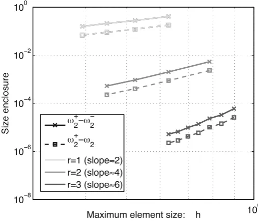
5 Convergence and error estimates
Our first goal in this section will be to show that, ifLcaptures an eigenspace of A within a certain order of precisionO(ε)as specified below, then the residuals
|t∓∓Fj(t∓)−n∓j(t)|
(see the right side of (12)) are
(a) O(ε)for anyt ∈R, (b) O(ε2)fort∈/σ(A).
This will be the content of Theorems13and14, and Corollary15. We will then show that, in turns, (24) has always residual of orderO(ε2)for anyt ∈R. See Theorem16. In the spectral approximation literature this property is known as optimal order of convergence/exactness, see [18, Chapter 6] or [33].
Recall Remark2, and the Assumptions1and2. Below{φtj}mj=1denotes an ortho-normal set of eigenvectors ofE[t−dm(t),t+dm(t)](A)which is ordered so that
|A−t|φtj =dj(t)φtj for j =1, . . . ,m.
Whenever 0< εj <1 is small, as specified below, the trial subspaceLwill be close
to Span{φtj}mj=1in the sense that there existwtj ∈Lsuch that
wt j −φ
t
j ≤εj and (A0)
|wt j−φ
t
j|t ≤εj. (A1)
We have split this condition into two terms, in order to highlight the fact that some times only (A1) is required. Unless otherwise specified, the index j runs from 1 to m. From Assumption2 it follows that the family{φsj}mj=1 ⊂ E[t−dm(t),t+dm(t)](A)
and the family{wsj}mj=1 ⊂Labove can always be chosen piecewise constant fors in a neighbourhood oft. Moreover, they can be chosen so that jumps only occur at s∈σ(A).
A set{wtj}mj=1subject to (A0)–(A1) is not generally orthonormal. However, accord-ing to the next lemma, it can always be substituted by an orthonormal set, provided
εjis small enough.
Lemma 12 There exists C >0independent ofLensuring the following. If{wtj}mj=1⊂
Lis such that(A0)-(A1)hold true for allεj such that
ε= m
j=1
ε2
j <
1
√
then there is a set{vtj}mj=1⊂Lorthonormal in the inner product·,·such that
|vt
j−φtj|t+ vtj−φtj<Cε.
Moreover,all these vectors are locally constant in t with jumps only at the spectrum of A.
Proof Recall Assumption2. As it is clear from the context, in this proof we suppress the indexton top of any vector. The desired conclusion is achieved by applying the Gram–Schmidt procedure. Let G = [wk, wl]klm=1 ∈ Cm×m be the Gram matrix
associated to{wj}. Set
vj = m
k=1
(G−1/2)k j wk.
Then
G−I ≤
m
k,l=1
|wk, wl − φk, φl|2
≤ 2
m
k,l=1
wk−φk2(wl + φl)2
≤√2(2+ε)ε.
Since
vj−wj2=
## ## #
m
k=1
(G−1/2−I)k jwk
## ## # 2
=
m
k,l=1
(G−1/2−I)k j(G−1/2−I)l jwk, wl
=
m
k=1
(G−1/2−I)k j
! m
l=1
Gkl(G−1/2−I)l j
"
=
m
k=1
(G−1/2−I)k j(G1/2−G)j k
=(I−G1/2)2
j j
then
AsG1/2is a positive-definite matrix, for everyv∈Cm we have
(G1/2+I)v2= G1/2v2+2G1/2v, v + v2≥ v2. Then det(I+G1/2)=0 and(I +G1/2)−1 ≤1. Hence
vj−wj ≤ (I−G)(I+G1/2)−1 ≤ I−G (I+G1/2)−1 ≤(2+ε)ε. (25)
Now, identifyv=(v1, . . . , vm)∈Cm withv=
m
k=1vkφk. As
G1/2v = ## ## ##
m
j=1
v, φjwj
## ##
##≥ v − ## ## ##
m
j=1
v, φj(wj−φj)
## ##
##≥(1−ε)v
then
G−1/2 ≤ 1 1−ε.
Hence
|vj −wj|t ≤ m
k=1
|(G−1/2−I)j k||wk|t
≤
m
k=1
|(G−1/2−I)j k|(εk+dk(t))
≤
m
k,l=1
|(G−1/2)kl||(G1/2−I)l j|(εk+dk(t))
≤ √
m(ε+dm(t))(2+ε)
1−ε ε. (26)
The conclusion follows from (25) and (26).
5.1 Convergence of the approximated local counting function
The next theorem addresses the claim (a) made at the beginning of this section. Accord-ing to Lemma12, in order to examine the asymptotic behaviour ofFj(t)asεj → 0
under the constraints (A0)–(A1), without loss of generality the trial vectorswtj can be assumed to form an orthonormal set in the inner product·,·.
Theorem 13 Let{wtj}mj=1 ⊂L be a family of vectors which is orthonormal in the inner product·,·and satisfies(A1).Then
Fj(t)−dj(t)≤
⎛ ⎝j
k=1
ε2
k
⎞ ⎠
1/2
Proof Recall Assumption2. From the Rayleigh–Ritz principle we obtain
Fj(t)≤max
|ck|2=1
j
k=1 ckwk
t
≤max
|ck|2=1
j
k=1
ck(wk−φk)
t
+max
|ck|2=1
j
k=1 ckφk
t
=max
|ck|2=1
j
k=1
ck(wk−φk)
t
+dj(t).
This gives
Fj(t)−dj(t)≤max
|ck|2=1
j
k=1
|ck||wk−φk|t
≤max
|ck|2=1 ⎛ ⎝j
k=1
|ck|2
⎞ ⎠
1/2⎛ ⎝j
k=1
|wk−φk|2t
⎞ ⎠
1/2
≤ ⎛ ⎝j
k=1
ε2
k
⎞ ⎠
1/2
as needed.
In terms of order of approximation, Theorem13will be superseded by Theorem14 fort∈/σ (A). However, ift ∈σ (A), the trial spaceLcan be chosen so thatF1(t)−d1(t) is only linear inε1. Indeed, fixing any non-zerou ∈D(A)andL=Span{u}, yields F1(t)−d1(t)= F1(t)=ε1. Therefore Theorem13is optimal, on the presumption thattis arbitrary.
The next theorem addresses the claim (b) made at the beginning of this section. Its proof is reminiscent of that of [29, Theorem 6.1].
Theorem 14 Let t ∈/σ (A). Suppose that theεjin(A1)are such that
m
j=1
ε2
j <
d1(t)2
6 . (27)
Then,
Fj(t)−dj(t)≤3d j(t)
d1(t)2
j
k=1
ε2
k ∀j =1, . . . ,m. (28)
Proof Recall Assumption2. Sincet ∈/σ(A), then(D(A),qt(·,·))is a Hilbert space.
Let PL:D(A)−→Lbe the orthogonal projection ontoLwith respect to the inner productqt(·,·), so that
Then|u|2t = |PLu|2t + |u−PLu|2t for allu ∈D(A)and|u−PLu|t ≤ |u−v|tfor all
v∈L. Hence
|φk−PLφk|t ≤εk ∀k=1, . . . ,m. (29)
LetEj =Span{φk}kj=1. Define
Fj = {φ∈Ej : φ =1} and
μj
L(t)=φmax∈Fj2 Reφ, φ−PLφ − φ−PLφ2.
HereμLj depends ont, asPLdoes. We first show that, under hypothesis (27),μLj(t) < 1
2. Indeed, givenφ∈Fj we decompose it asφ= j
k=1ckφk. Then
|φ, φ−PLφ| =
j
k=1
ckφk, φ−PLφ
= j
k=1 ck
dk(t)2
qt(φk, φ−PLφ)
= qt ⎛ ⎝ j
k=1 ck
dk(t)2φ
k, φ−PLφ
⎞ ⎠ = qt ⎛ ⎝ j
k=1 ck
dk(t)2(φ
k−PLφk), φ−PLφ
⎞ ⎠ ≤ j
k=1 ck
dk(t)2(φk−
PLφk)
t j
k=1
ck(φk−PLφk)
t
. (30)
For each multiplying term in the latter expression, the triangle and Cauchy–Schwarz’s inequalities yield (takeαk =ck orαk = ck
dk(t)2)
j
k=1
αk(φk−PLφk)
t ≤ j
k=1
|αk| |φk−PLφk|t
≤ ⎛ ⎝j
k=1
|αk|2
⎞ ⎠
1/2⎛ ⎝j
k=1
|φk−PLφk|2t
⎞ ⎠
1/2
. (31)
Then
|2 Reφ, φ−PLφ| ≤2 ⎛ ⎝
j
k=1
|ck|2
dk(t)4
⎞ ⎠
1/2⎛ ⎝
j
k=1
|ck|2
⎞ ⎠
1/2
j
k=1
ε2
k
≤ 2
d1(t)2
j
k=1
ε2
k (32)
The other term in the expression forμLj(t)has an upper bound found as follows. According to the Rayleigh–Ritz principle
φ−PLφ2≤ 1
d1(t)2
qt(φ−PLφ, φ−PLφ). (33)
Therefore, by repeating analogous steps as in (30) and (31), we get
φ−PLφ2≤ 1
d1(t)2
j
k=1
ckqt(φk−PLφk, φ−PLφ)
=qt
⎛ ⎝j
k=1 ck
d1(t)2
(φk−PLφk), φ−PLφ
⎞ ⎠
=qt
⎛ ⎝j
k=1 ck
d1(t)2(φk− PLφk),
j
l=1
cl(φl−PLφl)
⎞ ⎠
≤ 1
d1(t)2
j
k=1
ε2
k. (34)
Hence, from (32) and (34),
μj
L(t)≤ 3
d1(t)2
j
k=1
ε2
k <
1
2 (35)
as a consequence of (27).
Next, observe that dim(PLEj)= j. IndeedPLψ=0 forψ =1 would imply
μj
L(t)≥2 Reψ, ψ−PLψ − ψ−PLψ2= ψ2=1, which would contradict the fact thatμLj(t) <1. Then,
Fj(t)2≤ max u∈PLEj
|u|2t
u2 =maxφ∈E
j
|PLφ|2t
PLφ2 =φmax∈F
j
|PLφ|2t
PLφ2. As
PLφ2= φ2−2 Reφ, φ−PLφ + φ−PLφ2≥1−μLj(t), we get
Fj(t)2≤ max
φ∈Fj |φ|2
t
1−μLj(t) =max|ck|2=1 j
k=1|ck| 2
dk(t)2
1−μLj(t) =
dj(t)2
Finally, (36) and (35) yield
Fj(t)2−dj(t)2≤
μj
L(t) 1−μLj(t)dj(t)
2
≤2μLj(t)dj(t)2
≤2 3
d1(t)2d
j(t)2 j
k=1
ε2
k. (37)
The proof is completed by observing thatFj(t)+dj(t)≥2dj(t).
As the next corollary shows, a quadratic order of decrease for Fj(t)−dj(t)is
prevented for t ∈ σ (A)(in the context of Theorems13and14), only for j up to dimEt(A).
Corollary 15 Let t ∈σdisc(A),=1+dimEt(A)and k∈ {, . . . ,m}. Let
αk(t)=
1
4min{|dl(t)−dl−1(t)| :dl(t)=dl−1(t),l=, . . . ,k}>0. There exists ε > 0 independent of k ensuring the following. If(A1)holds true for
m
j=1ε2j < ε,then
Fk(t)−dk(t)≤3 dk(
t)
αk(t)2 k
j=1
ε2
j.
Proof Without loss of generality we assume thatt+dk(t)∈ σ (A). Otherwiset−
dk(t)∈σ(A)and the proof is analogous to the one presented below.
Lett˜ = t +αk(t). Then t˜ ∈/ σ(A)andt +dk(t) = ˜t +dk(t˜). Since the map
s → s+Fj(s)is non-decreasing as a consequence of Proposition2, Theorem14
applied att˜yields
Fk(t)−dk(t)=t+Fk(t)−(t+dk(t))≤ ˜t+Fk(t˜)−(t˜+dk(t˜))
=Fk(t˜)−dk(t˜)≤3dk(
˜
t)
d1(t˜)2
k
j=1
ε2
k ≤3
dk(t)
αk(t)2 k
j=1
ε2
j
as needed.
5.2 Convergence of local bounds for eigenvalues
and it allowst ∈σ(A). These two improvements are essential in order to obtain sharp bounds for those eigenvalues which are either degenerate or form a tight cluster.
Remark 4 The constantsε˜t andCt±below do have a dependence ont. This
depen-dence can be determined explicitly from Theorem14, Corollary15and the proof of Theorem16. Despite the fact that these constants can deteriorate ast approaches the isolated eigenvalues ofAand they can have jumps precisely at these points, they may be chosen independent ofton compact sets outside the spectrum.
Remark 5 By virtue of Corollary 11 and Corollary 6, τ−1
j(t) ≤ ν
−
j (t)− t and
1
τ+j (t) ≥ν
+
j(t)−t. Then
ˆ
t−j =t+ 1 2τ−j (t) ≤
t+ν−j(t)
2 ≤
ν+j (t)+ν−j(t)
2 ≤
ν+j (t)+t
2 ≤t+
1 2τ+j (t) = ˆt
+
j .
We regard the following as one of the main results of this work.
Theorem 16 Let J ⊂Rbe a bounded open segment such that J∩σ(A)⊆σdisc(A). Let{φk}mk˜=1be a family of eigenvectors of A such thatSpan{φk}mk˜=1=EJ(A). For fixed
t ∈ J such that Assumption1is satisfied,there existε˜t >0and Ct−>0independent
of the trial spaceL,ensuring the following. If there are{wj}mj˜=1⊂Lsuch that ⎛
⎝m˜
j=1
wj−φj2+ |wj −φj|2t
⎞ ⎠
1/2
≤ε <ε˜t, (38)
then
0< ν−j (t)− !
t+ 1
τ−j (t)
"
≤Ct−ε2
for all j ≤n−(t)such thatν−j (t)∈ J .
Proof The hypotheses ensure that the number of indices j ≤ n−(t) such that
ν−j (t) ∈ J never exceedsm. Therefore this condition in the conclusion of the the-˜
orem is consistent. Let
m(t)=max{m∈N: [t−dm(t),t+dm(t)] ⊂ J}.
The hypothesis on L guarantees that (A0)–(A1) hold true for m = m(t) and
(m
j=1ε2j)1/2 < ε. By combining Lemma12and Theorem13and the fact that we
can pick{wtj}mj=(t1)⊆ {wk}mk˜=1, there existsε˜t >0 small enough, such that (38) yields
Fj(s)−dj(s)≤
t−ν1−(t)
Let jbe such thatν−j (t)∈ J. Sinceν−j (t)−(α+t)≤(t+α)−ν1−(t)for allα such thatν
−
j(t)+ν1−(t)
2 −t ≤α≤0, then
dj(s)=s−ν−j(t) ∀s∈
ν1−(t)+ν−j(t)
2 ,
t+ν−j(t) 2
.
Let
g(α)=Fj(t+α)+α.
Thengis an increasing function ofαandg(0)=Fj(t) >0. For the strict inequality
in the latter, recall Assumption1. Moreover, according to (39),
g !
ν−j(t)+ν1−(t)
2 −t
" =Fj
!
ν−j (t)+ν1−(t) 2
"
−t+ν1−(t)−ν
−
1(t)−ν−j (t)
2
=Fj
!
ν−j (t)+ν1−(t) 2
"
−t+ν1−(t)−dj
!
ν−j(t)+ν1−(t) 2
"
≤ t−ν−1(t)
2 −(t−ν
−
1(t)) <0.
Hence, the intermediate value theorem ensures the existence ofα˜ ∈(ν −
1(t)+ν−j(t)
2 −t,0) such thatα˜ =Fj(t+ ˜α). According to Theorem10,α˜is unique andα˜ = 2τ−1
j (t)
.
The proof is now completed as follows. By virtue of Remark5,
ˆ
t−j (t)=t+ 1 2τ−j (t)∈
!
ν1−(t)+ν−j (t)
2 ,
t+ν−j (t) 2
"
and Fj(tˆ−j (t))=
1 2τ−j (t).
Then, Theorem14or Corollary15, as appropriate, ensure the existence ofCt− > 0
yielding
ν−j (t)−
! t+ 1
τ−j (t)
"
=Fj(tˆ−j )−dj(tˆ−j )≤Ct− j
k=1
ε2
k <C−t ε
2,
as needed.
5.3 Convergence to eigenfunctions
We conclude this section with a statement on convergence to eigenfunctions.