You are the only possible oracle: Effective test selection for end users of interactive machine learning systems

City, University of London Institutional Repository

Citation

:

Groce, A., Kulesza, T., Zhang, C., Shamasunder, S., Burnett, M., Wong, W-K,

Stumpf, S., Das, S., Shinsel, A., Bice, F. and McIntosh, K. (2014). You are the only possible

oracle: Effective test selection for end users of interactive machine learning systems. IEEE

Transactions on Software Engineering, 40(3), pp. 307-323. doi: 10.1109/TSE.2013.59

This is the unspecified version of the paper.

This version of the publication may differ from the final published

version.

Permanent repository link: http://openaccess.city.ac.uk/3620/

Link to published version

:

http://dx.doi.org/10.1109/TSE.2013.59

Copyright and reuse:

City Research Online aims to make research

outputs of City, University of London available to a wider audience.

Copyright and Moral Rights remain with the author(s) and/or copyright

holders. URLs from City Research Online may be freely distributed and

linked to.

You Are the Only Possible Oracle:

Effective Test Selection for End Users of

Interactive Machine Learning Systems

Alex Groce[1], Todd Kulesza[1], Chaoqiang Zhang[1], Shalini Shamasunder[1], Margaret Burnett[1],

Weng-Keen Wong[1], Simone Stumpf[2], Shubhomoy Das[1], Amber Shinsel[1], Forrest Bice[1],

Kevin McIntosh[1]

[1] School of Electrical Engineering and Computer Science

Oregon State University

Corvallis, Oregon 97331-3202

alex,kuleszto,zhangch,burnett,wong,[email protected]

[email protected], [email protected], [email protected], [email protected]

[2] Centre for HCI Design, School of Informatics

City University London

London EC1V 0HB, United Kingdom

[email protected]

Abstract—How do you test a program when only a single user, with no expertise in software testing, is able to determine if the program is performing correctly? Such programs are common today in the form of machine-learned classifiers. We consider the problem oftestingthis common kind of machine-generated program when the only oracle is anend user: e.g., onlyyoucan determine if your email is properly filed. We present test selection methods that provide very good failure rates even for small test suites, and show that these methods work in both large-scale random experiments using a “gold standard” and in studies with real users. Our methods are inexpensive and largely algorithm-independent. Key to our methods is an exploitation of properties of classifiers that is not possible in traditional software testing. Our results suggest that it is plausible for time-pressured end users to interactively detect failures—even very hard-to-find failures—without wading through a large number of successful (and thus less useful) tests. We additionally show that some methods are able to find the arguably most difficult-to-detect faults of classifiers: cases where machine learning algorithms have high confidence in an incorrect result.

Index Terms—machine learning; end-user testing; test suite size;

F

1

I

Machine learning powers a variety of interactive ap-plications, such as product recommenders that learn a user’s tastes based on their past purchases, “aging in place” systems that learn a user’s normal physical activity patterns and monitor for deviations, and in-terruptibility detectors on smart phones to decide if a particular incoming message should interrupt the user. In these settings, a machine learning algorithm takes as input a set of labeled training instances and produces as output a classifier. This classifier is the machine-generated output of a hand-written program, and is also a program in its own right.

This machine-generated program, like a human-written program, produces outputs for inputs that are provided to it. For example, a classifier on a user’s smart phone might take an incoming message and the user’s history and personal calendar as inputs and output a reason to interrupt or not (“work-critical

interruption”). Such classifiers, like other software artifacts, may be more or less reliable—raising the possibility that they are not reliable enough for their intended purposes.

A classifier can mislabel an input (fail) even if the algorithm that generated the classifier is correctly implemented. Failures occur for a variety of reasons such as noise in the training data, overfitting due to a limited amount of training data, underfitting because the classifier’s decision boundaries are not expressive enough to correctly capture the concept to be learned, and sample selection bias, where training instances are biased towards inputs uncommonly seen in real-world usage. Further, many machine learning systems areinteractive and continually learn from their users’ behavior. An interactive machine learning system may apply different output labels to the same input from one week to the next, based on how its user has recently interacted with the system.

effective testingof classifiers arises. That classifiers are created indirectly by another program, rather than directly by humans, does not obviate the need for testing, or remove the problem from the domain of software testing, but does affect who is in a position to test the system. Deployed classifiers can often be tested only by end users—sometimes, in fact, byonly one end user. For example, only you know which messages should interrupt you during a particular activity. Unfortunately, this means that for many clas-sifiers a unique situation arises: no individual with software development knowledge, or even a rudimen-tary understanding of testing, is in a position to test the system.

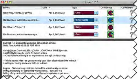
Given this problem, two issues arise: how to au-tomatically choose “good” test cases, and how to interact with end users while testing. This paper presents underlying algorithms for test case selection and data about how these methods perform, both ex-perimentally (by comparison with statistical sampling and hypothetical end user methods), and empirically with actual end users in a prototype interface (Figure 1). This paper adopts the distinction between experi-mentalandempiricalresults described by Harman et al. [24], and considers large-scale automated evaluations with benchmark data to be synthetic experiments and results with users and a concrete implementation and interface to be more empirical in nature (though also controlled experiments in a laboratory setting).

End-user testing of machine-generated classifiers is different from both machine learning’s “active learn-ing” (see Figure 2) [53] and from conventional soft-ware testing. The three main differences are depicted in Figure 2: (1) with active learning, the classifier

initiates the process, whereas with end-user testing, the user initiates the process; (2) with active learning,

Fig. 1. A user interface to allow end users to test a classifier [32]. This classifier takes a message (input) and produces a topic label (output). The pie chart depicts the classifier’s confidence that the message belongs in the red category (Cars), the blue category (Motorcycles), etc. A user can mark any message’s topic label as right or wrong; these marked messages are the test cases.

Active Learning Classifier Testing

Fig. 2. Active learning vs. classifier testing. The meth-ods differ in 1) whether the classifier or the user drives interaction, 2) the aim of instance selection (maxi-mize learning or maxi(maxi-mize bug-detection) and 3) the outcome of the process (a better classifier, or user knowledge of classifier quality).

learning is being optimized, whereas with end-user testing, failure detection is being optimized; and (3) with active learning, the intended outcome is a better

classifier, whereas with end-user testing, the intended outcome is betteruser insightinto where the classifier works correctly and where it does not.

End-user testing of classifiers also differs from con-ventional software testing: end users’ expertise at, and patience for, testing are likely lower than with professional programmers. Moreover, the software be-ing tested is different than conventional software in important ways, such as the structure of its (machine-generated) “source code” and the context in which it resides. Although these differences present challenges, they also provide opportunities unusual in testing (e.g., classifiers are often able to predict their own accuracy). We discuss the implications of these dif-ferences in detail in the next sections.

for SE” (Machine Learning for Software Engineering) systems are obviously far more expert at software development and testing than traditional end-users, they are still unlikely to be machine learning experts or have the patience or time to serve as oracles for a large set of test cases [52]. The methods introduced in this paper are therefore potentially important to the future of software engineering itself.

This paper encapsulates our previous work, which introduced a user interface (WYSIWYT/ML) [32] to support end users testing classifiers, and makes the following additional contributions:

• Formally frames a test selection problem.

• Proposes and formally defines three test selection

methods for this domain.

• Proposes a methodology for experimentally

eval-uating classifier testing methods for humans as a filtering process before costly user studies.

• Investigates our test selection methods in

large-scale automated experiments, over a larger vari-ety of benchmarks than possible with humans

• _{Evaluates which found failures are} unexpected_,

making them both especially challenging and important to detect, a problem difficult to explore in human studies.

Our experimental results show that our best test selection methods can produce very small test suites (5-25 instances) in which 80% of test cases fail (and thus expose faults), even when the tested classifier is 80% accurate. Our best methods find at least three times as many failures as random testing. Further, our results indicate that the high efficiency of our test methods is not attributable to finding many redun-dant failures identifying the same fault. Two of our methods are even able to find “surprise failures”, in which a classifier failsdespitehaving high confidence in its results. These methods also produce effective increases in the ability of end users to test a classifier in a short amount of time, with the ranking of meth-ods in basic agreement with our experimental results, suggesting that the experimental methods may be valid for exploring other approaches to the problem.

2

P

D

We first define the notion of end-user testing for machine-learned classifiers, loosely following the ap-proach taken by Rothermel et al. for end-user testing of spreadsheets [48].

Theprogramto be tested is a classifierC, a black box functioni→`, wherei∈I, the set of input instances, and`∈L, the set of all labels1_{. Classifiers decompose} the instances in I into features (e.g., text strings such as words) in a multi-dimensional space. Atest casefor classifierCis a tuple(i, `), wherei∈Iis the input (in

1. If we modifyC (e.g., retrain) we consider it a new program C0and assume no relationship between tests forC andC0.

this paper, a text message) and`∈Lis the label that classifierC assigns toi. A testis an explicit decision by the user that`’s value is correct or incorrect fori. Afailureof C is any test for which the user indicates that the label is incorrect.

2.1 The Test Selection Problem

Two common approaches to testing are test case generation and test selection. Test case generation (an algorithm producing inputs to test) is necessary when the creation of complex inputs (e.g., sequences of method calls) is required. In our setting, however, numerous inputs are often readily available: end users often have a large set of unlabeled instances in I

available for testing, e.g., the set of all unfiled emails in an inbox. Unlabeled instances can be converted to test cases simply by applying C to i to produce `. Therefore, the problem is usually one ofselectingtest cases to execute from a finite set of existing potential test cases. The expected use case of test selection is in an interface that brings to the user’s attention instances to test, whether in a stand-alone interface, or in the context of a “host” interface, e.g., messages in an email client.

2.2 What Is a Fault?

The IEEE Standard [1] defines a fault to be “an in-correct step, process, or data definition in a computer program.” This definition clearly applies to classifiers that mislabel outputs: from the user’s view, it has made a mistake. However, most of the literature assumes that a fault has a program location and so can be localized and fixed. This assumption is not so obviously true for a classifier, since faults are often tied to the training data itself, rather than to the lines of code that process training data.

heavily. Another approach is to allow users to add explicit rules to a classifier, such as with whitelists in spam identification—thus a fault can be localized to a missing or incorrect rule.

Thus, the definition of a “localizable” fault depends on the correction method: in traditional software test-ing, it is missing or incorrect code, while in classifiers it can be missing or incorrect training set data, feature labels, or rules, depending on the available debugging methods. Since the test selection methods in this paper are agnostic to the fault-correction method parameter, they do not attempt to localize the faults they reveal, but focus solely on detecting failures.

For simplicity, we will consider all failed test cases to be of equal cost. In some applications, such as in surveillance, false positives have a different cost than false negatives. We plan to incorporate these costs into our analysis in future work.

3

S

R

Because the problem of end users testing the clas-sifiers they have interactively customized has not been addressed in the literature, we offer a set of requirements for viability in this domain, used to formulate an evaluation process for candidate test selection methods.

3.1 Requirements for Viability

End-user testing of classifiers has a number of dif-ferences from conventional software testing. In this section, we discuss how three of these differences impose non-traditional requirements.

The first difference is the nature of the software (a classifier) itself. Traditional code coverage approaches to testing are unsatisfying because a classifier’s “code” contains only a small portion of the classifier’s logic: the behavior is generally driven by parameters (data) derived from the training set. Further, improved al-gorithms and underlying mathematical bases are fre-quently introduced; thus, even if a “code+data” cover-age approach could be customized for one algorithmic approach (e.g., decision trees), it would be likely to be completely unsuited to another (e.g., support vector machines). These issues suggest an algorithm-independent approach: Requirement: A testing method for a classifier should be agnostic to the machine learning algorithm that performs the classification.

Second, the software infrastructure hosting an end user’s classifier is usually highly interactive, pro-viding immediate feedback even if the classifier changes—e.g., a spam filter may change every time new email arrives, and classify spam slightly dif-ferently from one moment to the next. Hence the following:Requirement: The testing method must be fast enough to run in the interactive environment the user is accustomed to using (e.g., if the classifier sorts email, then the testing method would run in an email client).

Third, the end-user-as-oracle situation points out a crucial limitation: the user’s patience, and thus the number of test cases that users will be willing to judge in testing the classifier. Prior work with spreadsheet users’ testing practices suggests that end users are willing to judge only a small number of test cases, perhaps fewer than 10. Panko explains this low rate by pointing out that low levels of testing can be self-reinforcing [45]: by not carefully testing, users can perceive benefits by saving time and avoiding onerous work. Further, when they do catch errors informally, these errors can further convince users of their efficacy in error correction without the need for more rigor. Even scientific users are unlikely to find testing more than a few tens of instances a worthwhile use of their time [52]. Therefore, we impose:Requirement: Effective failure detection must be achieved with a small test suite, one or more orders of magnitude smaller than in regular testing practice.

This third requirement has an interesting nuance because, as with human-created software systems, it is not the case that all failures (and faults) are equally important. In more traditional software development efforts, “bug triage” can be a problem, both in the de-velopment of tests (in order to focus on finding critical faults) and after failures are found. With classifiers, where it is expected that even the highest quality clas-sifiers will sometimes fail to correctly classify some instances, this is perhaps an even more important aspect of the testing.

To see why, consider the following. Although most classifiers “know” when they lack enough informa-tion to be certain of the label for an instance—a trait we use to our advantage in our test selection methods, as discussed in the next section—this ability to self re-flect may sometimes be misleading. A classifier might correctly point out a possible failure when the proba-bility assigned to the chosen label is low (perhaps due to a lack of training data similar to that instance, or ambiguity between two classes). However, a classifier may also have misplaced confidence in output labels that are wrong. Cases in which the classifier has high confidence in an incorrect labeling ` may be of particular importance in testing; they may be the prime targets for hand debugging [60], or reveal larger problems with the training set or with assumptions made by the classifier. These failures are a surprise given the classifier’s high confidence—hence we call themsurprisefailures.

3.2 Research Questions

Our overall research question is simple: “How do you find the most failures made by a classifier while exam-ining the fewest outputs?”. We explored this question in two parts—first via an experimental study using a wide range of classifiers, data sets, and test set sizes, and then via an empirical user study to discover if the same experimental findings hold when we introduce end users into the loop. These two objectives were broken down into seven research questions:

• _{RQ1 (Efficiency):} Which proposed testing

meth-ods produce effective test suites for a user?

• RQ2 (Accuracy variation):Does test method

ef-fectiveness vary with classifier accuracy? (i.e., Do we need different testing methods for accurate vs. inaccurate classifiers?)

• RQ3 (Algorithm variation):Do the most effective

test methods generalize across multiple learning algorithms and data sets?

• RQ4 (Surprise failure detection): Are “surprise

failures” (failures that the learning algorithm was confident were correct) identified by the same test methods used to identify non-surprise failures, or are different test methods required for this class of failures?

• _{RQ5 (User Efficacy):} Will end users, when

pro-vided with efficient testing methods, find more failures than viaad hoctesting?

• RQ6 (User Efficiency):Can a test coverage

mea-sure help end users to test more efficiently than

ad hoctesting?

• RQ7 (User Satisfaction): What are end users’

attitudes toward systematic testing as compared toad hoctesting?

4

T

S

C

M

-ODS

Our methods include bothtest case prioritizations [14] and coverage metrics. A prioritization strategy, given a set of test cases, orders them according to some criterion. We can then select a test suite of size n

by taking the top n ranked test cases. Thus, even if users do not evaluate the full suite, they are at least testing the items with the highest priority (where

priority depends on the purpose of the test suite, e.g., finding common failures, or finding surprising failures). A coverage measure evaluates a test suite based on some measure: e.g., branches taken, partition elements input, or mutants killed.

The first three test case selection methods we describe, CONFIDENCE, COS-DIST, and LEAST-RELEVANT, are the methods we had reason to propose (pre-evaluation) as potential candidates for actual use. In addition, we describe three “base-line” methods, MOST-RELEVANT, CANONICAL, and RANDOM, to provide a context for understand-ing the performance of the proposed methods. We also

propose a test coverage metric based upon the COS-DIST selection method.

Our general problem statement makes no assump-tions on the structure of instancesi, labels`, or classi-fiersC, but our methods assume that it is possible to measure a distance (measure of similarity) between two instances, d(i1, i2) and that a classifier can

pro-duce, in addition to a labeling for an instance, a

confidence(estimated probability that a label is correct), so that a test case becomes a tuple (i, `, p), where p

is the classifier’s estimate of P(` correct for i). We also assume that we can compute information gain on features. These requirements generally hold for most commonly used classification algorithms.

4.1 Determining Test Coverage

Our proposed method for determining test cover-age of a machine-generated classifier is rooted in the notion ofsimilarity. Because classifiers attempt to categorize similar inputs together (where “similar” is defined by the specific features the classifier uses for categorization), inputs that are similar to many items in the training set are likely to be correctly cat-egorized. Conversely, inputs that are unlike anything in the training set are likely to pose a problem for the classifier—it may not know how to categorize such items because it has never seen anything like them before. Once a user had indicated that an input was correctly classified, it may be possible to assume that sufficiently similar inputs will also be correctly classified.

Thus, we propose that test coverage in this domain is a function of how similar each test case is to the untested inputs. For example, take a classifier that has made 10 predictions, nine of which involve inputs that are very similar to one another (and are all predicted to haveLabel A), and one input which is unlike any of the others (and is predicted to have Label B). If a user were to test any one of the first nine inputs and found it to be correct, we can hypothesize that the remaining eight are also correct—the classifier is likely using the same reasoning to classify all of them. However, this tells us nothing about the tenth input, because its categorization may be informed by different reasoning within the classifier (e.g., rules generalized from different training instances). Thus, our user’s test coverage would be 90%. Conversely, if she tested only the tenth item, her test coverage would be 10%. Via this metric, a user would need to test at least one item from each cluster of similar items to achieve 100% test coverage.

is incorrect for the ninth item, it does not necessarily tell us anything about the other eight inputs. Thus, we propose that for a user’s test of input i1 to also

cover input i2, i1 and i2 must be sufficiently similar

(as defined by some distance measure d(i1, i2)) and

share the same output label`.

4.2 Proposed Test Selection Methods

CONFIDENCE Prioritization:

From a software testing perspective, CONFI-DENCE, a method based on prioritizing test cases in ascending order ofpin(i, `, p)(such that cases where the label has the lowest probability are tested first), is analogous to asking the software’s original pro-grammer to prioritize testing code most likely to fail— but in our case, the “programmer” is also software. Thus, the CONFIDENCE approach is a prioritization method that capitalizes on the ability of classifiers to “find their own bugs” by selecting cases where they have low confidence.

Confidence can be measured in a variety of ways. We compute confidence as the magnitude of the probability assigned to the most likely labeling, and prioritize test cases according to those with the lowest probabilities2_{. CONFIDENCE selects ambiguous test} instances—instances that fall on or close to decision boundaries. Most machine learning algorithms can compute this measure of confidence in some form; most commonly, it is the conditional probability of the label`given the instance i’s features.

Thus, CONFIDENCE largely satisfies the require-ment that methods bealgorithm-agnostic(Section 3.1). Computing confidence is also computationally inex-pensive, as it is “built-in” to most classifiers. However, this prioritization method also requires time at least linear in the size of the test instance universe; this can be reduced in the case of unusually large sets by random sampling.

Despite the apparently high potential of this method, one problem with this approach concerns the quality of confidence estimates. For example, can clas-sifiers with low accuracy evaluate their own spheres of competence? Even highly accurate classifiers may not have well-calibrated confidence measures. A sec-ond problem is that the CONFIDENCE method will— almost by definition—fail to find surprise failures.

COS-DIST Prioritization:

COS-DIST prioritizes tests in descending order of their average cosine distance d(i, t) to all members t

2. We also evaluated a similar prioritization based on uncertainty sampling, but omit the results as this method generally performed slightly worse than CONFIDENCE.

of the training set3_{. Instances most distant from the} training set are tested first. From a software testing perspective, COS-DIST is analogous to prioritizing test cases that might fail because they are “unusual”. The underlying assumption is that test cases most unlike the training set are likely to fail.

In principle, the idea of prioritizing test cases based on distance could apply to many software systems. What is unusual is (1) the existence of the training set, to provide a baseline notion of “typical” cases for which the software is expected not to fail, and (2) a continuity and statistically based form of behavior that gives us hope that simple, easily computable distance metrics on inputs will be relevant to behavior. In more typical testing, computing useful distances between test cases is problematic: two API calls may invoke very different software behavior despite dif-fering only slightly.

This testing method is clearly algorithm-agnostic, since it rests solely on the contents of the training set. Computing distances between large training sets and large test sets takes time proportional to the product of the sizes of the sets, but as with CONFIDENCE, random sampling can be used for approximate results. Regarding our third requirement (effective failure detection with small test suites), COS-DIST avoids two of the potential shortfalls of CONFIDENCE be-cause it does not use a classifier’s opinion of its own competence. However, this method shares with CONFIDENCE the potential problem that focusing on finding likely-to-fail test cases seems unlikely to reveal surprise failures.

LEAST-RELEVANT Prioritization:

The two methods above are potentially heavily bi-ased against surprise failures. The LEAST-RELEVANT method attempts to solve that problem. From a soft-ware testing perspective, LEAST-RELEVANT is analo-gous to selecting test cases that might fail because they don’t take any of the most common paths through the code. Its key motivation is the premise that failure may be more likely for instances lacking the “most important” features.

Suppose an enumeration is available of the k fea-tures (e.g., words in the input documents) most rel-evant to making classifications. In our experiments, we use information gain (over the entire universe of instances) to measure feature relevance; another possibility is for the user to tell the classifier which features are most relevant [35]. Given this set, LEAST-RELEVANT ranks a test case (i, `) by the absence of these key features in the instance (fewer key features results in higher prioritization). Because the set may

be user-provided, we have limited our results to con-sideringk=20 features. In a sense, LEAST-RELEVANT shares the same goals as COS-DIST, but hopes to avoid over-selecting for outlier instances by using a coarse binary distinction, balancing failure detection with the ability to find surprise failures.

LEAST-RELEVANT is agnostic to the underlying machine learning algorithm, but may become imprac-tical for classification problems with a small number of features. In such a case, it may be more useful to prioritize tests based on a lack of discriminative feature values (e.g., a scalar feature may be discrim-inative if its value is less than 10, but ambiguous otherwise) rather than a lack of discriminative fea-tures themselves. LEAST-RELEVANT also feafea-tures a computation cost proportional to the test suite size.

Regarding the third requirement, identifying fail-ures with an extremely small test set, our premise is that the degree to which an input lacks relevant features may correlate with its chance of failure. For surprise failures, we predict that LEAST-RELEVANT will be less biased against surprise failures than confidence-based and distance-based methods.

4.3 Baseline Test Selection Methods

To experimentally evaluate our proposed testing methods, we needed baseline methods that might be intuitively attractive to end users in the absence of more systematic prioritizations. In evaluations with actual users, user behavior in the absence of assistance served as a true baseline.

MOST-RELEVANT Coverage:

The MOST-RELEVANT coverage metric (the in-verse of LEAST-RELEVANT) is based on the notion of “covering” features that are most relevant to classifica-tion. We include it because users might want to focus on features that matter most to them. In traditional software testing terms, this seems somewhat analo-gous to testing “usual” cases. Ranking is determined as in LEAST-RELEVANT, but increases with presence

of the most relevant features, rather than with their absence.

CANONICAL Prioritization:

If attempting to test “systematically” without guid-ance from a testing system, a user might test an archetypal example (or examples) for each label. We simulate this notion of canonicity by grouping in-stances according to their true label and then calcu-lating the centroid of each set. For each set, we take the instances closest to the centroid as canonical. We test canonical instances for each class in proportion to the appearances of that class (classes with many instances contribute more instances). In traditional testing terms, this method is similar to choosing test cases for each specification of desired output.

RANDOM:

RANDOM testing is potentially a competitive base-line method. Although once considered to be some-thing of a strawman, in recent years the effectiveness of random testing has been shown to be competi-tive with more systematic methods when it can be applied to software testing [3]. Further, its statistical heritage is an excellent match for the statistical nature of classifiers, suggesting special suitability to this domain. Even if we expect systematic methods to improve on random testing in terms of effectiveness, random testing lacks the dangerous potential bias against finding surprise failures that is a disadvantage for our proposed methods above. Random testing is (statistically) guaranteed to find such failures at a rate roughly equivalent to their actual prevalence.

5

E

E

5.1.1 Procedures and Data

We evaluated our test selection methods over classi-fiers based on randomly chosen training sets ranging from 100 to 2,000 instances, in increments of 100. For each training set size, we generated 20 training sets and produced classifiers for each training set, reserving all items not used in training as potential test case instances; thus I is the set of all data set instances not used to train C, the classifier to be tested. Varying training set size is an indirect method of controlling classifier accuracy; larger training sets usually produce more accurate classifiers. Finally, we applied each test selection method to each classifier, selecting test cases fromI, for test suite sizes ranging from 5 to 25 instances, in increments of 5 (recall our requirement of very small test suites). For LEAST-RELEVANT, MOST-LEAST-RELEVANT, and RANDOM, we generated five test suites for each training set (LEAST and MOST relevant result in many ranking ties, which we settled randomly). For more fine-grained priority-based methods, we needed only one test suite for each training set, as the results were deterministic. The original labeled data sets served as test oracles:`was correct when it matched the label foriin the original data set.

To produce multiple classifiersCto test, we trained a Naive Bayes (NB) classifier [40] and a Support Vector Machine (SVM) [12] on each training set. These two types of classifiers were chosen because they are commonly used machine learning algorithms for text data. We used the Mallet framework [41] and LIBSVM [8] to produce classifiers and to perform distance, information gain, and confidence calculations. For SVM classifiers, confidence is computed based on the second method proposed by Wu et al. [61], the default approach in LIBSVM.

were: “20 Newsgroups” [36], “Reuters-21578” [4], and the “Enron data set” [55]. For 20 Newsgroups data we used the set which contains 11,293 newsgroup docu-ments divided into 20 categories. The Reuters data set contains 5,485 news stories, labeled by subject; we used only the 8 most common categories. The Enron set (for userfarmer) consists of 3,672 emails divided into 25 categories.

5.1.2 Evaluation Measures

To answer Research Questions 1–3, we report each method’sefficiency: the number of failures divided by the total number of tests.

To answer Research Question 4, (determining which methods are most likely to find the most surprising

failures), we use a sliding surprise threshold to re-port each method’s detection of incorrect results in which the classifier’s confidence exceeded a certain threshold. The sliding threshold avoids an arbitrary choice, allowing us to consider all values above 0.5 to be potential definitions of the “surprise” level. (Below 0.5, the classifier is saying it has at least a 50/50 chance of being wrong—hardly constituting a surprising failure.)

5.2 Results

5.2.1 Testing Efficiency

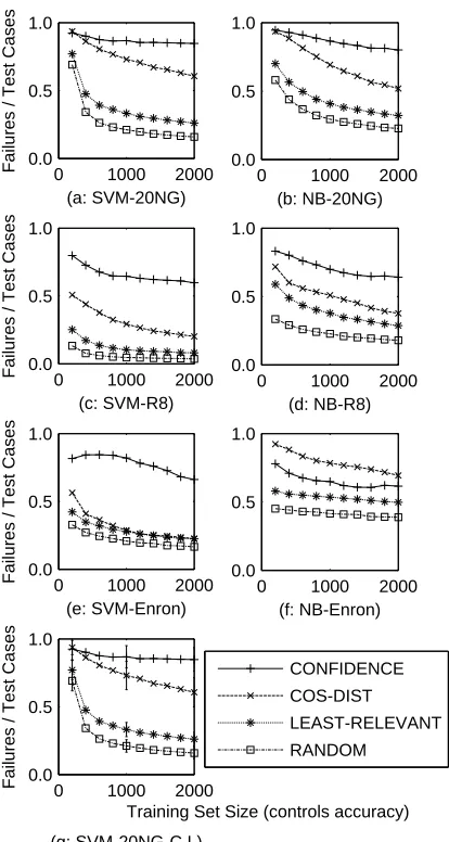
Our three proposed testing methods were all sig-nificantly more efficient than RANDOM in all ex-perimental configurations. (We show only RANDOM in comparison to our proposed methods, as it out-performed the other baseline methods.) The CONFI-DENCE method performed best in five of the six con-figurations, with COS-DIST second best in those five. (CONFIDENCE and COS-DIST switched places in the sixth configuration.) LEAST-RELEVANT showed the least improvement over the RANDOM baseline. Fig-ure 3 graphs these differences: the efficiencies shown are averages of rates over all suites (whose sizes ranged from 5 to 25 test cases) and all classifiers at each training set size. For all but the smallest training sets (200–500 instances), differences between all pairs of methods, except where data points coincide, are significant at the 95% confidence level.4 _{Figure 3(g)} shows 95% confidence intervals at three training set sizes of Figure 3(a)’s configuration5.

As the Figure 3 illustrates, the best methods were very efficient at identifying failures. For example, consider the RANDOM line in Figure 3(c). RANDOM is statistically guaranteed to detect failures at the rate they occur, and thus is also a statistical representative of the classifier’s accuracy. This indicator shows that

4. Confidence intervals were computed over all runs for each training set size, in standard statistical practice [59].

5. Other sizes were similar but omitted for readability; some of the intervals are so tight that they are almost occluded by the data points.

0 1000 2000

0.0 0.5 1.0

(a: SVM-20NG)

F

a

ilur

e

s / T

e

st Cases

0 1000 2000

0.0 0.5 1.0

(b: NB-20NG)

0 1000 2000

0.0 0.5 1.0

(c: SVM-R8)

F

a

ilur

e

s / T

e

st Cases

0 1000 2000

0.0 0.5 1.0

(d: NB-R8)

0 1000 2000

0.0 0.5 1.0

(e: SVM-Enron)

F

a

ilur

e

s / T

e

st Cases

0 1000 2000

0.0 0.5 1.0

(f: NB-Enron)

0 1000 2000

0.0 0.5 1.0

(g: SVM-20NG-C.I.)

F

a

ilur

e

s / T

e

st Cases

0 10002000 0.0

0.5

1.0 CONFIDENCE COS-DIST

LEAST-RELEVANT RANDOM

Training Set Size (controls accuracy)

Fig. 3. Failure detection effectiveness in different clas-sifiers: All three methods outperformed RANDOM, with CONFIDENCE usually in the lead except for (f). (a-b): 20 Newsgroups by SVM (a) and Naive Bayes (b). (c-d): Reuters by SVM and Naive Bayes. (e-f): Enron by SVM and Naive Bayes. (g): SVM-20NG’s confidence intervals at three training set sizes (200, 1000, and 2000).

this challenge—it performed almost as well with very accurate classifiers (rightmost x-values in Figure 3) as with very inaccurate classifiers (leftmost x-values).

The data sets and algorithms across these experi-ments cover three very different situations classifiers face. The 20 Newsgroups data set (Figure 3(a-b)) pro-duced classifiers challenged by ambiguity, due largely to the “Miscellaneous” newsgroups. The Reuters data set (Figure 3(c-d)), with only a few classes, produced classifiers under a nearly ideal setting with many sam-ples from each class. The Enron configuration (Figure 3(e-f)) produced classifiers challenged by the problem of class imbalance, with folders ranging in size from about 10 to over 1,000. Despite these differences, the ranks of the methods were identical except for the CONFIDENCE/COS-DIST swap in Figure 3(f).

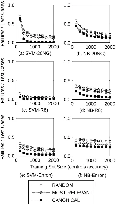
In contrast to the three proposed methods, the methods we believe match what users might “in-tuitively” do (CANONICAL and MOST-RELEVANT) did not usually perform better than RANDOM (Fig-ure 4), and sometimes performed significantly worse. The reason for this inefficiency is that the “most typ-ical” instances and those containing the most useful keywords for classification are precisely the instances even poor classifiers are most likely to label correctly. Thus, the “intuitive” methods cannot fulfill our third requirement.

In these experiments, differences in size of our small test suites (5 vs. 10 vs. ... 25 test cases) rarely seemed to matter; thus we do not provide data for each size because the results were so similar. The two highest performing methods (CONFIDENCE and COS-DIST) did show a mild degradation in efficiency as suite size increased, further evidence of the effectiveness of prioritization in those two methods.

By the standards of the software testing literature, where popular methods such as branch coverage are only weakly correlated with fault detection [17], [18], all three are effective testing methods, especially CONFIDENCE and COS-DIST. In software testing, strategies strongly correlated with suite effectiveness (independent of suite size) tend to be very expensive to evaluate and less useful as test generation or selec-tion methods (e.g., mutaselec-tion testing or all-uses testing [18]). In contrast, our approaches are computationally inexpensive and effective for selecting even very small test suites.

5.2.2 Surprise Failures

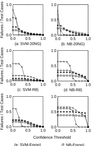
Identifying surprise failures—cases in which the clas-sifier is confident in its erroneous labeling—caused the relative order of our methods’ performance to change. Figure 5 illustrates how methods run into difficulty as the degree of a failure’s “surprisingness” (confidence) increases along the x-axis. The x-axis begins at no surprisingness at all (confidence at zero). As noted, we do not consider failures at confidence

0 1000 2000

0.0 0.5 1.0

(a: SVM-20NG)

F

a

ilur

e

s / T

e

st Cases

0 1000 2000

0.0 0.5 1.0

(b: NB-20NG)

0 1000 2000

0.0 0.5 1.0

(c: SVM-R8)

F

a

ilur

e

s / T

e

st Cases

0 1000 2000

0.0 0.5 1.0

(d: NB-R8)

0 1000 2000

0.0 0.5 1.0

(e: SVM-Enron)

F

a

ilur

e

s / T

e

st Cases

0 1000 2000

0.0 0.5 1.0

(f: NB-Enron)

RANDOM

MOST-RELEVANT

CANONICAL

Training Set Size (controls accuracy)

Fig. 4. Failure detection effectiveness of the base-line techniques. Both “intuitive” basebase-line methods per-formed worse than RANDOM. The classifiers shown are (a-b): 20 Newsgroups by SVM (a) and Naive Bayes (b). (c-d): Reuters by SVM and Naive Bayes. (e-f): Enron by SVM and Naive Bayes.

below 0.5 to be surprising, thus surprises are on the right side of these graphs.

The graphs shown are for the most accurate clas-sifiers (i.e., those trained on 2,000 instances), because failures in cases of high confidence by these accurate classifiers constitute the most surprising of all failures. Classifiers trained on smaller trainings sets showed similar results.

As Figure 5 shows, CONFIDENCE, though highly efficient at low levels of classifier confidence, lost all effectiveness by the right half of the graphs. The drop occurred earlier in SVM than in Naive Bayes, possibly because of Naive Bayes’s propensity toward over-confidence [63]. We expected the baseline CANON-ICAL and MOST-RELEVANT methods to do well at finding surprise failures because they tend to select high-confidence labelings, but they performed poorly; perhaps their poor ability to detect failures overall prevented success at detecting this kind of failure.

of-0.0 0.5 1.0 0.0

0.5 1.0

(a: SVM-20NG)

F

a

ilur

e

s / T

e

st Cases

0.0 0.5 1.0

0.0 0.5 1.0

(b: NB-20NG)

0.0 0.5 1.0

0.0 0.5 1.0

(c: SVM-R8)

F

a

ilur

e

s / T

e

st Cases

0.0 0.5 1.0

0.0 0.5 1.0

(d: NB-R8)

0.0 0.5 1.0

0.0 0.5 1.0

(e: SVM-Enron)

F

a

ilur

e

s / T

e

st Cases

0.0 0.5 1.0

0.0 0.5 1.0

(f: NB-Enron) Confidence Threshold

Fig. 5. Failure detection with confidence thresholds, at training set size 2,000 (the x-axis is the confidence level of the classifier). CONFIDENCE performed poorly as the confidence threshold increased, but COS-DIST and LEAST-RELEVANT outperformed RANDOM. (a-b): 20 Newsgroups by SVM (a) and Naive Bayes (b). (c-d): Reuters by SVM and Naive Bayes. (e-f): Enron by SVM and Naive Bayes. (Legend is same as Figure 3.)

ten identifying them at a significantly higher rate than they actually occurred (as represented by the RAN-DOM line). Its superiority held over a range of levels of surprise (i.e., the right half of the x-axis). Figure 5(b)’s 20 Newsgroups data set with Naive Bayes was the only configuration where COS-DIST performed poorly. We hypothesize that its poor performance in this case was due to the overlap in newsgroup contents, which caused most of the failures to be due to ambiguity and thus lie near decision boundaries. Data instances that are very far away from the training set (according to COS-DIST) may be well inside a decision boundary and thus correctly classified.

At all thresholds for surprise (thresholds from 0.5 to 0.9), COS-DIST found surprise failures significantly better than RANDOM in three configurations (Fig-ure 5(a), (c), and (f)), with significance calculated as in Section 5.2.1. LEAST-RELEVANT significantly im-proved on RANDOM at some surprise thresholds in configurations (b) and (f). Differences between COS-DIST and LEAST-RELEVANT were also significant in

0.0 0.5 1.0

0 1000 2000

Failures / Test Cases

Training Set Size (controls accuracy)

CONFIDENCE COS-DIST LEAST-RELEVANT RANDOM

Fig. 6. After removing items that might expose “the same fault” (by distance), CONFIDENCE and COS-DIST approaches still performed very well.

configurations (a), (b), (c), and (f), with COS-DIST better in all but the aforementioned (b) case.

We are encouraged and surprised that any testing methods performed well for surprise failures in any of the classifiers, because the methods that succeeded overall (recall Figure 3) all work by seeking outliers— the very instances for which a classifiershouldexhibit low confidence. We attribute the success of COS-DIST and LEAST-RELEVANT to their focus on finding

unusual rather than ambiguous instances (as found by CONFIDENCE). It appears that using COS-DIST provides a good balance between finding a high quantity of failures and finding the elusive surprise failures, and may be the testing method of choice when considering both the quality and quantity of failures found.

5.2.3 Regarding Test Coverage, and Grouping Fail-ures by Similarity

A potential explanation for our best methods’ per-formance could have been that they selected many similar test cases that all expose “the same fault” (under many correction methods). To check for this possibility, given that it is not possible to define “faults” without all the necessary parameters (Section 2.2), we considered the following assumption: failing instances that are similar (by distance metric thresh-old) to each other are more likely to expose the same fault. We tested this assumption for both SVM and Naive Bayes as follows: we added failing instances (with correct labels `) to the training set, generated new classifiers, and examined the changes.

The results supported our assumption. For both SVM and Naive Bayes, items similar to the failing test’s instance, when compared to randomly selected instances, were, after retraining: (1) more likely to change classification, (2) less likely to change to an incorrect labeling, and (3) roughly twice as likely to change from an incorrect to a correct labeling. This indicates that the notion of using distance as a surrogate for “exposes same fault” likelihood is not unreasonable.

prioritized item for each set of similar items (thus, in most cases, testing many lower-priority items than in the original results). The resulting failure detection efficiency for our best methods was at worst only moderately degraded, and sometimes marginally im-proved: Figure 6 shows the results for an SVM on the 20 Newsgroups dataset, and is typical of other classi-fiers and datasets. This suggests that the effectiveness of our methods is not a result of detecting multiple instances of the same fault.

The above results also support our hypothesis that classifier test coverage can be reliably determined by assuming the classifier will treat similar items in a similar manner; we will further investigate the utility of this metric in the next section.

6

U

S

The results in Section 5 suggest that systematic testing of machine-generated classifiers can be done effec-tively and efficiently, but will actual users behave in such an ideal manner? To find out, we designed a framework (initially presented in [32]) to support end-user testing of an interactive machine learning system, and studied how end users worked with it.

6.1 What You See is What You Test

Our framework was loosely inspired by the What-You-See-Is-What-You-Test (WYSIWYT) approach of Rothermel et al. [48]; we thus dubbed it WYSI-WYT/ML (ML for machine learning). Like the origi-nal WYSIWYT system, our framework performs four functions: (1) itadvises (prioritizes) which predictions to test, (2) itcontributestests, (3) itmeasures coverage, and (4) it monitors for coverage changes. How it achieves this functionally, however, is unique to the domain of interactive machine learning.

WYSIWYT/ML supports two cases of users inter-acting with a classifier. In use case UC-1, can a user

initially rely on the classifier to behave as expected? For example, will a new email client correctly identify junk mail while leaving important messages in your inbox? By prioritizing tests, WYSIWYT/ML can help a user quickly identify which messages are most likely to be misclassified, and by contributing tests (via the coverage metric), it keeps the number of test cases a user must manually examine low. The coverage metric also informs the user how well-tested the classifier is, allowing him or her to determine how closely it needs to be monitored for mistakes (e.g., important email ending up in the junk mail folder).

In use caseUC-2, a user wants to know if his or her classifier is still reliable. Because interactive machine learning systems continue to learn post-deployment, there is no guarantee that a system that was reliable in the past will continue to perform as expected in the future. Thus, WYSIWYT/ML’s fourth function: mon-itoring for coverage changes. Coverage may change

because new inputs arrive that are unlike anything the user has yet tested, or the classifier’s reasoning may change, causing items the user previously indicated to be correctly classified to now have a new (and incorrect) output label.

6.2 Instantiating WYSIWYT/ML

We prototyped WYSIWYT/ML as part of a text-classifying intelligent agent. This agent took news-group messages and classified them by topic (a screen-shot is shown in Figure 1). Thus, testing this agent involved determining whether or not it had classified each message correctly.

6.2.1 Advising Which Predictions to Test

Our prototype prioritizes the classifier’s topic pre-dictions that are most likely to be wrong, and com-municates these prioritizations using saturated green squares to draw a user’s eye (e.g., Figure 1, fourth message). The prioritizations may not be perfect, but they are only intended to be advisory; users are free to test any messages they want, not just ones the system suggests. We created three variants of the WYSIWYT/ML prototype, each using one of the pri-oritization criteria identified in Section 4.2: CONFI-DENCE, COS-DIST, and LEAST-RELEVANT.

WYSIWYT/ML’s implementation of the CONFI-DENCE selection criteria displays classifier confidence to the user (and allows the user to sort on confidence). The higher the uncertainty, the more saturated a green square (Figure 1, Confidence column). Within the square, WYSIWYT/ML “explains” CONFIDENCE prioritizations using a pie chart (Figure 7, left). Each pie slice represents the probability that the message belongs to that slice’s topic: a pie with evenly sized slices means the classifier thinks each topic is equally probable (thus, testing it is a high priority).

The COS-DIST method is implemented via a “fish-bowl” that explains this method’s priority, with the amount of “water” in the fishbowl representing how unique the message is compared to messages on which the classifier trained (Figure 7, middle). A full fishbowl means the message is very unique (com-pared to the classifier’s training set), and thus high priority.

The LEAST-RELEVANT method uses the number of relevant words (0 to 20) to explain the reason for the message’s priority (Figure 7, right), with the lowest numbers receiving the highest priorities.

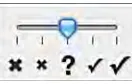
6.2.2 Contributing Tests and Measuring Coverage When a user wants to assess the classifier, he or she can pick a message and judge (i.e., test) whether the predicted topic is correct. Users can pick any message: one of WYSIWYT/ML’s suggestions, or some different message if he or she prefers. The user communicates this judgment by clicking a 3if it is correct or a7if it is incorrect, as in Figure 8 (smaller3 and7marks were available to indicate “maybe right” and “maybe wrong”, respectively). If a topic prediction is wrong, the user has the option of selecting the correct topic— our prototype treats this as a shortcut for marking the existing topic as “wrong”, making the topic change, and then marking the new topic as “right”.

WYSIWYT/ML thencontributesto the user’s testing effort: after each user test, WYSWYT/ML automati-cally infers the same judgment upon similar messages. These automated judgments constituteinferred tests.

To contribute these inferred tests, our approach computes the cosine similarity of the tested message with each untested message sharing the same pre-dicted topic. WYSWYT/ML then marks very simi-lar messages (i.e., scoring above a cosine simisimi-larity threshold of 0.05, a value established during pilot tests) asapprovedordisapprovedby the prototype. The automatically inferred assessments are shown with gray3and7marks in the Correctness column (Figure 9, top), allowing users to differentiate their own ex-plicit judgments from those automatically inferred by WYSIWYT/ML. Of course, users are free to review (and if necessary, fix) any inferred assessments—in fact, most of our study’s participants started out doing exactly this.

WYSIWYT/ML’s third functionality is measuring

test coverage: how many of the classifier’s predictions have been tested by Adam and the inferred tests together. A test coverage bar (Figure 9, bottom) keeps users informed of this measure, helping them decide how much more testing may be warranted.

6.2.3 Monitoring Coverage

Whenever a user tests one of the classifier’s predic-tions or new content arrives for the prototype to classify, the system immediately updates all of its information. This includes the classifier’s predictions (except for those a user has “locked down” by explic-itly approving them), all testing priorities, all inferred tests, and the test coverage bar. Thus, users can always

Fig. 8. A user can mark a predicted topic wrong, maybe wrong, maybe right, or right (or “?” to revert to untested). Prior research found these four choices to be useful in spreadsheet testing [21].

see how “tested” the classifier is at any given moment. If a user decides that more testing is warranted, he or she can quickly tell which predictions WYSIWYT/ML thinks are the weakest (UC-1) and which predictions are not covered by prior tests (UC-2).

6.3 Experimental Methodology

We conducted a user study to investigate use-case UC-1, the user’s initial assessment of a classifier. This study was designed to investigate Research Questions 5, 6, and 7.

We used three systematic testing treatments, one for each prioritization method (CONFIDENCE, COS-DIST, and LEAST-RELEVANT). We also included a fourth treatment (CONTROL) to representad hoc test-ing. Participants in all treatments could test (via3,7, and label changes) and sort messages by any column in the prototype. See Figure 1 for a screenshot of the CONFIDENCE prototype; COS-DIST and LEAST-RELEVANT looked similar, save for their respective prioritization methods and visualizations (Figure 7). CONTROL supported the same testing and sorting actions, but lacked prioritization visualizations or in-ferred tests, and thus did not need priority/inin-ferred test history columns. CONTROL replaces our hypoth-esized CANONICAL and MOST-RELEVANT meth-ods, as well as RANDOM, in that it represents actual user behavior in the absence of an automated selec-tion/prioritization method.

The experiment design was within-subject (i.e., all participants experienced all treatments). We randomly selected 48 participants (23 males and 25 females) from respondents to a university-wide request. None of our participants were Computer Science majors, nor had any taken Computer Science classes be-yond the introductory course. Participants worked with messages from four newsgroups of the 20 Newsgroups dataset [31]: cars, motorcycles, computers,

and religion (the original rec.autos, rec.motorcycles, comp.os.ms-windows.misc, and soc.religion.christian newsgroups, respectively).

We randomly selected 120 messages (30 per topic) to train a support vector machine [8]. We randomly selected a further 1,000 messages over a variety of dates (250 per topic) and divided them into five data sets: one tutorial set (to familiarize our participants with the testing task) and four test sets to use in the study main tasks. Our classifier was 85% accurate when initially classifying each of these sets. We used a Latin Square design to counterbalance treatment orderings and randomized how each participant’s test data sets were assigned to the treatments.

Participants answered a background questionnaire, then took a tutorial to learn one prototype’s user interface and to experience the kinds of messages and topics they would be seeing during the study. Using the tutorial set, participants practiced testing and finding the classifier’s mistakes in that prototype. For their first task, participants used the prototype to test and look for mistakes in a 200-message test set. They then filled out a Likert-scale questionnaire with their opinions of their success, the task difficulty, and their opinions of the prototype. They then took another brief tutorial explaining the changes in the next prototype variant, practiced, and performed the main task using the next assigned data set and treat-ment. Finally, participants answered a questionnaire covering their overall opinions of the four prototypes and comprehension. Each testing task lasted only 10 minutes.

6.4 Experimental Results

6.4.1 RQ5 (User Efficacy): Finding Failures

To investigate how well participants managed to find a classifier’s mistakes using WYSIWYT/ML, we com-pared failures they found using the WYSIWYT/ML treatments to failures they found with the CONTROL treatment. An ANOVA contrast against CONTROL showed a significant difference between treatment means (Table 1). For example, participants found nearly twice as many failures using the frontrunner, CONFIDENCE, than using the CONTROL version.

Not only did participants find more failures with WYSIWYT/ML, the more tests participants per-formed using WYSIWYT/ML, the more failures they found (linear regression, F(1,46)=14.34, R2_=.24,b=0.08,

p<.001), a relationship for which there was no evidence in the Control variant (linear regression, F(1,45)=1.56, R2_{=.03, b=0.03, p=.218). Systematic}

test-ing ustest-ing WYSIWYT/ML yielded significantly better results for finding failures than ad-hoc testing.

Our formative offline oracle experiments revealed types of failures that would be hard for some of our methods to target as high-priority tests. (Recall that, offline, LEAST-RELEVANT and COS-DIST were

better than CONFIDENCE in this respect.) In order to evaluate our methods with real users, we took a close look at Bug 20635, which was one of the hardest failures for our participants to find (one of the five least frequently identified). The message topic should have been Religion but was instead predicted to be Computers, perhaps in part because Bug 20635’s message was very short and required domain-specific information to understand (which was also true of the other hardest-to-find failures):

Subject: Mission Aviation Fellowship

Hi, Does anyone know anything about this group and what they do? Any info would be appreciated. Thanks!

As Table 2 shows, nearly all participants who had this failure in their test set found it with the LEAST-RELEVANT treatment, but a much lower fraction found it using the other treatments. As the table’s Pri-oritization column shows, LEAST-RELEVANT ranked the message as very high priority because it did not contain any useful words, unlike CONFIDENCE (the classifier was very confident in its prediction), and unlike COS-DIST (the message was fairly similar to other Computer messages). Given this complemen-tarity among the different methods, we hope in the future to evaluate a combination (e.g., a weighted average or voting scheme) of prioritization methods, thus enabling users to quickly find a wider variety of failures than they could using any one method alone.

6.4.2 RQ6 (User Efficiency): The Partnership’s Test Coverage

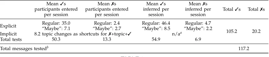
Using WYSIYWT/ML, our participants were able to more than double their test coverage. Together with the computer-oracle-as-partner, participants’ mean of 55 test actions using WYSIWYT/ML covered a mean of 117 (60%) of the messages—thus, participants gained 62 inferred tests “for free”. Table 3 shows the raw counts. With the help of their computer partners, two participants even reached 100% test coverage, covering all 200 messages within their 10-minute time limit.

Further, coverage scaled well. In an offline experi-ment, we tried our participants’ explicit tests on the

entireset of Newsgroup messages from the dates and topics we had sampled for the experiment—a data set containing 1,448 messages. (These were tests partici-pants explicitly entered using either WYSIWYT/ML or CONTROL, a mean of 55 test actions per ses-sion.) Using participants’ explicit tests, the computer inferred a mean of 568 additional tests per participant, for a total coverage of 623 tests (mean) from only 10 minutes of work—a 10-fold leveraging of the user’s invested effort.

Mean (p-value for contrast with Control)

df F p

CONFIDENCE COS-DIST LEAST-RELEVANT Control

Failures found (max 30) 12.2 (p<.001) 10.3 (p<.001) 10.0 (p<.001) 6.5 (n/a) 3,186 10.61 <.001 Helpfulness (max 7) 5.3 (p<.001) 5.0 (p<.001) 4.6 (p<.001) 2.9 (n/a) 3,186 22.88 <.001 Perceived success (max 21) 13.4 (p=.016) 13.3 (p=.024) 14.0 (p=.002) 11.4 (n/a) 3,186 3.82 .011

TABLE 1

ANOVA contrast results (against Control) by treatment. The highest values in each row are shaded.

Treatment Prioritization Found Did not find

CONFIDENCE 0.14 9 15

COS-DIST 0.58 11 14

LEAST-RELEVANT 1.00 19 4

TABLE 2

The number of participants who found Bug 20635 while working with each WYSIWYT/ML treatment.

Mean3s participants entered

per session

Mean7s participants entered

per session

Mean3s inferred per

session

Mean7s inferred per

session

Total3s Total7s

Explicit Regular: 35.0_{“Maybe”: 7.1 “Maybe”: 2.7}Regular: 2.4 Regular: 46.4_{“Maybe”: 8.5 “Maybe”: 2.2}Regular: 4.7

105.2 20.2 Implicit 8.2 topic changes as shortcuts for7+topic+3 n/aa

Total tests 50.3 13.3 54.9 6.9

Total messages testedb 117.2

TABLE 3

Tests via3marks,7marks, and topic changes during a 10-minute session (out of 200 total messages per session), for the three WYSIWYT/ML treatments.

a. Although the computer sometimes did change topics, this was due to leveraging tests as increased training on message classification. Thus, because these topic changes were not directly due to the coverage (cosine-similarity) mechanism, we omit them from this coverage analysis.

b.Total testsis larger thanTotal messages testedbecause topic changes acted as two tests: an7on the original topic, then a3

on the new topic.

topic) for 94% of their regular checkmarks and 81% of their “maybe” checkmarks (the agreement level across both types of approval was 92%). By the same measure, WYSIWYT/ML’s approvals were also very accurate, agreeing with the gold standard an average 92% of the time—exactly the same level as the partic-ipants’.

Participants’ regular7marks agreed with the gold standard reasonably often (77%), but their “maybe” 7 marks agreed only 43% of the time. Informal pi-lot interviews revealed a possible explanation: re-appropriation of the “maybe” 7 marks for a subtly different purpose than it had been intended for. When unsure of the right topic, pilot participants said they marked it as “maybe wrong” to denote that itcouldbe wrong, but with the intention to revisit it later when they were more familiar with the message categories. This indicates that secondary notation (in addition to testing notation)—in the form of a “reminder” to revisit instead of a disapproval—could prove useful in future prototypes.

Perhaps in part for this reason, WYSIWYT/ML did not correctly infer many bugs—only 19% of its

7 marks agreed with the gold standard. (The com-puter’s regular 7 marks and “maybe” 7 marks did not differ—both were in low agreement with the gold standard.) Because WYSIWYT/ML’s regular inferred 7 marks were just as faulty, the problem cannot be fully explained by participants repurposing “maybe” 7marks. However, this problem’s impact was limited because inferred 7 marks only served to highlight

possiblefailures. Thus, the 81% failure rate on WYSI-WYT/ML’s average of seven 7 marks per session meant that participants only had to look at an extra five messages per session. Most inferred tests were the very accurate3marks (average of 55 per session), which were so accurate, participants could safely skip them when looking for failures.

6.4.3 RQ7 (User Satisfaction): Attitudes Towards Systematic Testing

Participants appeared to recognize the benefits of sys-tematic testing, indicating increased satisfaction over

that responses differed between treatments (Table 1, row 2), with WYSIWYT/ML treatments rated more helpful than Control. Table 1’s 3rd row shows that participant responses to the NASA-TLX questionnaire [26] triangulate this result. Together, these results are encouraging from the perspective of the Attention Investment Model [6]—they suggest that end users can be apprised of the benefits (so as to accurately weigh the costs) of testing a classifier that does work important to them.

7

D

We emphasize that finding (not fixing) failures is WYSIWYT/ML’s primary contribution toward debug-ging. Although WYSIWYT/ML leverages user tests as additional training data, simply adding training data is not an efficient method fordebuggingclassifiers. To illustrate, our participants’ testing labeled, on average, 55 messages, which increased average accuracy by 3%. In contrast, participants in another study that also used a subset of the 20 Newsgroup dataset spent their 10 minutes debugging by specifying words/phrases associated with a label [60]. They entered only about 32 words/phrases but averaged almost twice as much of an accuracy increase (5%) in their 10 minutes. Other researchers have similarly reported that allow-ing users to debug by labelallow-ing a word/phrase is up to five times more efficient than simply labeling training messages [46].

Thus, rather than attempting to replace the de-bugging approaches emerging for interactive ma-chine learning systems (e.g., [33], [35], [57]), WYSI-WYT/ML’s bug-finding complements them. For ex-ample, WYSIWYT/ML may help a user realize that an e-mail classifier often mistakenly labels messages about social networks (e.g., friend requests, status updates) as SPAM; the user could then use a feature labeling approach (e.g., [60]) to adjust the classifier’s reasoning. After such feedback, WYSIWYT/ML helps the user understand whether the classifier’s mistakes have been corrected, as well as whether new mis-takes have been introduced. WYSIWYT/ML provides a missing testing component to interactive machine learning systems; it suggests where important bugs have emerged and when those bugs have been erad-icated, so that end users need not debug blindly.

Our empirical evaluation showed that systemati-cally testing with WYSIWYT/ML resulted in a signif-icant improvement overad hocmethods in end users’ abilities to assess their classifiers: our participants found almost twice as many failures with our best WYSIWYT/ML variant as they did while testing ad hoc. Further, the approach scaled: participants covered 117 messages in the 200-message data set (over twice as many as they explicitly tested) and 623 messages in the 1448-message data set (over 10 times as many as they explicitly tested)—all at a cost of only 10 minutes work.

Thus, systematic assessment of machine-generated classifiers was not only effective at finding failures— it also helped ordinary end users assess a reason-able fraction of an classifier’s work in a matter of minutes. These findings strongly support the via-bility of bringing systematic testing to this domain, empowering end users to judge whether and when to rely on interactive machine learning systems that support critical tasks. These results also validate our experimental evaluations, in that they suggest that our proposed methodology can predict the relative performance of methods for actual users. However, the absolute performance differences between meth-ods were considerably smaller with human subjects than when performing purely automated testing. If the advantages of the non-CONFIDENCE methods for finding surprise faults carry over to the WYSI-WYT/ML setting (which we cannot currently claim to have statistically validated, due to the rarity of surprise faults in reasonable-sized test sets), the argu-ment for preferring other methods to CONFIDENCE may be stronger than our experimental evaluation would suggest.

8

T

V

We conducted experiments using two types of ma-chine learning classifiers (naive Bayes and a Support Vector Machine) and three datasets. However, there are many different machine learning techniques, and some operate quite differently than the classifiers we evaluated (e.g., decision trees, neural networks). Fur-ther, the three datasets we used in our evaluation may not be representative of all types of text-based classi-fication, and certainly do not tell us anything about testing machine learning systems on non-textual data (e.g., image recognition).

Our experimental evaluation used training set sizes of up to 2,000, but the datasets we explored contained many more items than that (up to 11,293). Thus, a different sample of training items may have resulted in different classifiers, and thus different failures. This is especially applicable at small training set sizes (e.g., 100 items), where variance between classifiers trained on different samples from a larger population is known to be high [7].