Numerical study of flapping filaments in a uniform fluid flow

City, University of London Institutional Repository

Citation

:

10.1016/j.jfluidstructs.2014.11.010

This is the accepted version of the paper.

This version of the publication may differ from the final published

version.

Permanent repository link: http://openaccess.city.ac.uk/6933/

Link to published version

:

Copyright and reuse:

City Research Online aims to make research

outputs of City, University of London available to a wider audience.

Copyright and Moral Rights remain with the author(s) and/or copyright

holders. URLs from City Research Online may be freely distributed and

linked to.

Numerical study of flapping filaments in an uniform

fluid flow

Julien Faviera,∗

, Alistair Revellb_{, Alfredo Pinelli}c

a

Aix Marseille Universit´e, CNRS, Centrale Marseille, M2P2 UMR 7340, 13451, Marseille, France.

b

School of Mechanical, Aerospace and Civil Engineering (MACE), University of Manchester, United Kingdom.

c

School of Engineering and Mathematical Sciences (EMS), City University, London, United Kingdom.

Abstract

The coupled dynamics of multiple flexible filaments (also called monodimen-sional flags) flapping in a uniform fluid flow is studied numerically for the cases of a side-by-side arrangement, and an in-line configuration. The modal behaviour and hydrodynamical properties of the sets of filaments are studied using a Lattice Boltzmann - Immersed Boundary method. The fluid momen-tum equations are solved on a Cartesian uniform lattice while the beating filaments are tracked through a series of markers, whose dynamics are func-tions of the forces exerted by the fluid, the filaments flexural rigidity and the tension. The instantaneous wall conditions on the filaments are imposed via a system of singular body forces, consistently discretised on the lattice of the Boltzmann equation. The results exhibits several flapping modes for two and three filaments placed sid-by-side and are compared with experimental and theoretical studies. The hydrodynamical drafting, observed so far only experimentally on configurations of in-line flexible bodies, is also revisited numerically in this work, and the associated physical mechanism is identi-fied. In certain geometrical and structural configuration, it is found that the upstream body experiences a reduced drag compared to the downstream body, which is the contrary of what is encountered on rigid bodies (cars, bicycles).

∗_{Corresponding author}

Keywords: beating filaments, flapping flags, inverted hydrodynamic drafting, Immersed Boundary, Lattice Boltzmann

1. Introduction

The scope of this work is the physical analysis of the dynamics of flap-ping filaments in a streaming ambient fluid, which has a large spectrum of applications in aeronautics, civil engineering or biological flows. From the theoretical side, this fluid structure interaction problem is particularly chal-lenging as it involves non-linear effects as well as large structural deformations (Pa¨ıdoussis, 2004; Shelley and Zhang, 2011). The present study is particu-larly inspired by various experiments on flapping filaments realised in soap films (Zhang et al., 2000; Zhu and Peskin, 2000; Ristroph and Zhang, 2008). Indeed, soap film experiments associated to thin-film interferometry for flow visualisation can be considered as a reasonable approximations of 2D fluid structure interaction scenarios, thus suitable for the validation of the results obtained with our 2D numerical approach.

In our simulations, we consider a 2D incoming incompressible flow mod-eled using a Lattice Boltzmann method, coupled to a model of infinitely thin and inextensible filament experiencing tension, gravity, fluid forces and flex-ural rigidity (i.e. a bending term in the form of a 4th derivative with respect to the curvilinear coordinate describing the filament). Also, at all time in-stants tension forces are determined to maintain the inextensibility of the structure. In this simple model the energy balance of the system is driven by the bending forces and fluid forces, as the structure is controlled by an inextensibility constraint which prohibits stretching or elongation motions that would dissipate energy. This system encompasses all the essential ingre-dients of a complex fluid-structure interaction problem: large deformations, slender flexible body, competition between bending versus fluid forces, inex-tensibility and effect of the filament tips on the surrounding flow as vorticity generators.

computationally cheap and directly provides for the forces exerted on the fluid by the filaments without the introduction of any empirical parameter. Using the Lattice Boltzmann method in conjunction with an Immersed Boundary technique to solve the motion of an incompressible fluid also allows for a clean imposition of the boundary conditions on the solid since it does not suffer from errors originating from the projection step, as it is the case when associated with unsteady incompressible Navier Stokes solvers (Domenichini, 2008).

Making use of the outlined Lattice Boltzmann - Immersed Boundary ap-proach, we consider the coupled dynamics of systems made of highly de-formable flexible filaments, as introduced by Favier et al. (2014). No artifi-cial contact force is introduced between the filaments, in order to preserve a purely hydrodynamical interaction. We focus in this work on the modal behaviour of a set of two and three side-by-side filaments, by varying the spacing between them. The obtained results confirm the theoretical predic-tions and experimental observapredic-tions mentioned in literature. Additionally, the drag reducing properties of multiple in-line filaments is studied, as a function of their relative spacing. In particular, the anomalous the so-called anomalous hydrodynamic drafting pointed out experimentally in Ristroph and Zhang (2008) is recovered here numerically and a physical mechanism is proposed to explain this phenomenon.

2. Coupled Lattice Boltzmann - Immersed Boundary Method

This fluid-structure problem is tackled using an Immersed Boundary method coupled with a Lattice Boltzmann solver. In the following we provide a summary of the numerical technique while details of the methodology can be found in Favier et al. (2014).

time t with particle velocity vectore is given as follows:

fi(x+ei∆t, t+ ∆t)−fi(x, t) =−

∆t

τ f(x, t)−f

(eq)_{(x, t)}

+ ∆tFi (1)

In this formulation, xare the space coordinates, ei is the particle velocity in

the ith _{direction of the lattice and F}

i accounts for the body force applied to

the fluid, which conveys the information between the fluid and the flexible structure. The local particle distributions relax towards an equilibrium state f(eq) _{in a single time scale τ. Equation 1 governs the collision of particles}

relaxing toward equilibrium (first term of the r.h.s.) together with their streaming which drives the data shifting between lattice cells (l.h.s of the equation). The rate of approach to equilibrium is controlled by the relaxation time τ, which is related to the kinematic viscosity of the fluid by ν = (τ ₋ 1/2)/3. Equation 1 is approximated on a Cartesian uniform grid by assigning to each cell of the lattice a finite number of discrete velocity vectors. In particular, we use the D2Q9 model, which refers to two-dimensional and nine discrete velocities per lattice node (corresponding to the directions east, west, north, south, center, and the 4 diagonal directions as given by equation 2), where the subscript i refers to these discrete particle directions. As is usually done, a convenient normalization is employed so that the spatial and temporal discretization in the lattice are set to unity, and thus the discrete velocities are defined as follows:

ei =c

0 1 ₋1 0 0 1 ₋1 1 ₋1

0 0 0 1 ₋1 1 ₋1 ₋1 1

(i= 0,1, ...,8) (2)

where c is the lattice speed which defined by c= ∆x/∆t = 1 with the cur-rent normalization. The equilibrium function f(eq)_{(x, t) can be obtained by}

Hermite series expansion of the Maxwell-Boltzmann equilibrium distribution (Qian et al., 1992):

f_i(eq)=ρωi "

1 + ei·u c2

s

+(ei·u)

2 2c4 s − u 2 2c2 s # (3)

In equation 3, cs is the speed of sound cs = 1/

√

3 and the weight coefficient ωi areω0 = 4/9,ωi = 1/9, i= 1...4 andω5 = 1/36, i= 5...8 according to the

This stands as the equivalent of the CFL number for classical Navier Stokes solvers. The force Fi in equation 1 is computed using a power series in the

particle velocity with coefficients that depend on the actual volume force fib

applied on the fluid. The latter is determined using the Immersed Boundary method, originally introduced by Peskin (2002), following the formulation described in Uhlmann (2005) for classical Navier Stokes solvers and Favier et al. (2014) for Lattice Boltzmann solvers. In this approach, the flexible filaments are discretised by a set of markers Xk, that in general do not

correspond with the lattice nodesxi,j. The role offibis to restore the desired

velocity boundary values on the immersed surfaces at each time step. The global algorithm is decomposed as follows. The Lattice-Boltzmann equations for the fluid are first advanced to the next time step without im-mersed object (Fi = 0), which provides the distribution functions fi needed

to build a predictive velocity up _{by ρu}p ₌ P i

eifi and ρ = P

i

fi. The

pre-dictive velocity is then interpolated onto the structure markers, which allows one to derive the forcing required to impose the desired boundary condition at each marker using:

Fib(Xk) =

Udn+1_(X

k)− I[up](Xk)

∆t (4)

In equation 4, capital letters are used to identify variables defined on each marker and _I[up_](X

k) refers to the interpolated predictive velocity. The term Udn+1_(X

k) denotes the velocity value at the location Xk we wish to obtain at time step completion. Adding this force term to the right hand side of the momentum equations allows to restore the desired velocity Udn+1 at the boundary (see Uhlmann (2005) for instance). The value of Udn+1 _is determined for each filament and at each Lagragian point by integrating in time the respective dynamic equation:

dUdn+1

dt =

∂ ∂s(T

∂Xk

∂s )−KB ∂4_X

k

∂s4 +Ri

g

g −Fib (5)

Here, the Richardson number isRi=gL/U2

∞,T is the tension of the filament

and KB is the flexural rigidity. All variables are non dimensional and the

reference quantities used for the normalisation are: the reference force tension

Tref = ∆ρU∞2 , the reference bending rigidity KB ref = ∆ρU 2

∞L2 _{and the}

reference Lagrangian forcing Fref = _ερ∆ρ

fU 2

thickness of the filament on the lattice. More details can be found in Favier et al. (2014). The closure of equation 5 is provided by the inextensibility condition that reads:

∂Xk

∂s · ∂Xk

∂s = 1 (6)

This condition, that ensures that the filament does not stretch (and thus its length remains constant), is satisfied using the tension values that effectively act as Lagrange multipliers. The boundary conditions for the system (5-6)

are X =X0,

∂2_X

k

∂s2 = 0 for the fixed end and T = 0,

∂2_X

k

∂s2 = 0 for the free

end.

Returning to equation 4, the term _I[up_](X

k) refers to the value of the

predictive velocity field interpolated at Xk. This provides the kinematic

compatibility between solid and fluid motion, i.e. zero relative velocity on the solid boundary. At this stage, the required forcing is known at each marker by equation 4, and needs to be spread onto the lattice neighbours by: fib(x) =S(Fib(Xk)).

More details on the interpolation operator _I, spreading operator _S and the filaments equations of motion can be found in Favier et al. (2014). With respect to literature, this approach of immersed boundary preserves an order 2 in space and ensures a conservation of the force and torque between Eulerian and Lagrangian space, for a relatively low computational cost. The forcing fib is finally discretised on the lattice directions and reads (Malaspinas, 2009;

Guo et al., 2002):

Fi =

1₋ 1 2τ

ωi

ei−u

c2

s

+ei·u c4

s

ei

·fib (7)

Once the system of hydrodynamic forces has been determined following the outlined procedure, equation 1 is then solved once again with the forcing Fi which impose the correct boundary condition at each markerXk. Finally,

the macroscopic quantities are then derived from the obtained distribution functions f by ρu=P

i

eifi+ρ∆₂tFand ρ=P i

fi, which closes one time step

of the solver.

3. One single flapping filament in an incoming fluid flow

filament fixed at one end, and subject to gravity and hydrodynamics forces. Let L be the length of the filament, we fix the density difference between solid and fluid ∆ρ = ρs −ρfL to ∆ρ = 1.5, the non-dimensional bending

rigidity to KB = 0.001, and the value of the Richardson number toRi= 0.5.

The inlet velocity imposed in the Lattice-Boltzmann normalization is set to U∞ = 0.04 (aligned with gravity direction), with a relaxation time of

τ = 0.524 and a filament length ofL= 40. With these values, the simulation is run at a Reynolds number Re = U∞L/ν equal to 200. The size of the

computational domain is set to 15L_×10L, in the streamwise and transverse direction respectively. The lattice discretization (600_×400 nodes) has been determined as the result of a preliminary grid convergence study. The initial angle of the filament is set to θ = 18o _{with respect to the gravity direction,}

and its fixed end is placed at the centerline of the domain, at a distance of 4L from the inlet. The L2 norm of the inextensibility error is kept below 10−12

at all times.

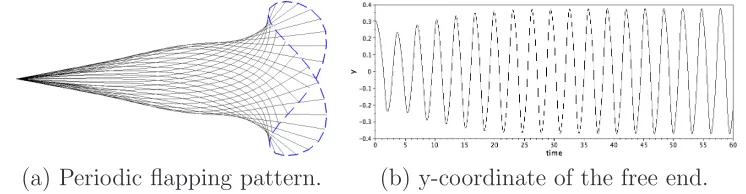
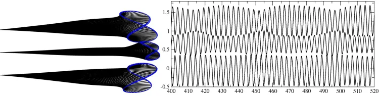
(a) Periodic flapping pattern. (b) y-coordinate of the free end.

Figure 1: Flapping motion of a single filament immersed in fluid atRe = 200,Ri= 0.5, ∆ρ= 1.5. Fluid flows from left to right. (a): beating pattern visualised by superimposed positions of the filament over one beating cycle. (b) Periodic time evolution of the y-coordinate of the free end.

free end exhibiting a characteristicfigure-eight orbit (dashed line in 1a) is re-covered, in agreement with the findings of the soap film experiments carried out by Zhang et al. (Zhang et al., 2000).

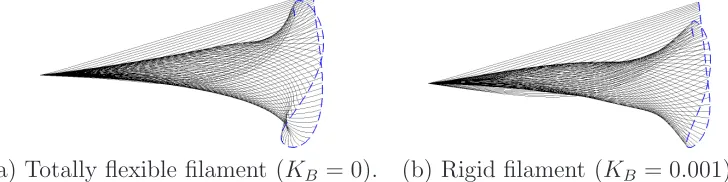
(a) Totally flexible filament (KB = 0). (b) Rigid filament (KB = 0.001).

Figure 2: Comparison between instantaneous snapshots of the flapping filament without bending (a) and with bending (b) starting from a straight initial configuration at an angle ofθ0= 18

o

. The trajectory of the free end is shown in dashed line.

Figures 2a and 2b show the effect of the bending rigidity coefficient on the beating pattern. Without bending rigidity (figure 2a), the filament is totally flexible and a rolling up of the free extremity is observed; this effect has been termed askick following Bailey (2000). On the other hand, when the filament has a finite flexural rigidity (KB = 0.001 in this simulation), the rolling up

of the free end is inhibited, the kick disappears and the flapping amplitude is reduced. Thus, the proposed slender structure model, incorporating both bending terms and tension, computed to enforce inextensibility, reproduces successfully the same phenomena as the ones observed in experiments.

4. Side-by-side flapping flaps

We now consider the case of two filaments in aside-by-sideconfiguration at Re = 300. The non-dimensional values, the domain size and the initial angles (θ = 18o_{) are kept the same as in the case of the single beating filament.}

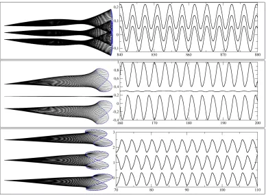
Figure 3: Snapshots of iso-vorticity for the case of two beating filaments atRe= 300 and three different spacings. (a) mode M1 atd/L= 0.1, (b) mode M2 atd/L= 0.3, (c) mode M2 at d/L= 1.0.

Therefore, in this context we have considered various scenarios corresponding to different values of the spacing d/L.

Figure 3 displays the snapshots of iso-vorticity that we predict when con-sidering three different spacings. The wakes are characterised by a periodic vortex shedding and by a flapping motion of the filaments (shown in fig-ure 4 for the three cases). The variations of the relative spacings between the filaments lead to different physical scenarios that are briefly reviewed hereafter.

filaments, as displayed in figure 4a.

• In contrast, when increasing the distance to d/L = 0.3, a different behaviour is observed. This mode (mode M2) is characterised by sym-metrical out-of-phase oscillations, occurring after a transient period which occurs between t = 20 and t = 60 (see figure 4b). By increas-ing the filament spacincreas-ing, the lock-in effect weakens but the interaction between the wakes generated by each filament still plays a dominant role, as shown in figure 3b. In this regime, the fluid enclosed between the filaments behaves like a flow generated by a pump due to the out-of-phase flapping, cyclically being compressed when the two free ends approach (which is the case of the snapshot displayed in figure 3b), and released when they move apart.

• Further increasing the spacing to d/L = 1 results in a further wear-kening of the wake interaction and a decoupling of the vortex streets behind the filaments (see figure 3c). However, beyond 5L downstream of the filaments tails, the vortices merge into a unique wake and the filaments reach the mode M2 characterised by an out-of-phase flapping (see figure 4c).

• If the spacing d/L is further increased, the two filaments eventually reach a totally decoupled dynamics with an in-phase flapping (mode M1).

The modal behaviour is consistent with the experimental observations of Zhang et al. (2000) that report the onset of the anti-phase regime at d/L = 0.21, compared to our numerical predictions indicating a transitory regime occurring between d/L = 0.21 and d/L = 0.24. Note that for a sufficiently fine discretisation, the duration of this transcient is independent of the mesh refinement.

Retaining the same Reynolds numberRe= 300, the configuration of three filaments placed side-by-side at an initial angle of 0o _{is investigated. Figure 5}

summarizes the different coupled dynamics obtained with the present simula-tions. The system follows the same behaviour as for the case of two filaments, except that an additional beating mode appears:

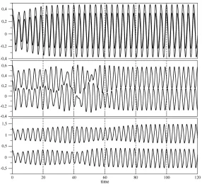
Figure 4: Time evolution of the y-coordinates of the free extremity of a system of two beating filaments at Re = 300. (a) Mode M1 atd/L= 0.1, (b) Mode M2 atd/L= 0.3, (c) Mode M2 atd/L= 1.0.

• ford/L= 0.3, the two outer filaments flap out of phase while the inner filament is quasi stationnary (mode M2 in figure 5b);

• for large spacing (d/L= 1.0) the outer filaments flap in-phase and the inner filament is out of phase (mode M3 in figure 5c);

• as for the case of two filaments, mode M1 is observed for very large spacing (d/L >4.0) with an in-phase flapping of the three filaments.

Figure 5: Flapping patterns in the established regime for the beating of three filaments in a uniform flow for various spacing. (a) mode M1 at d/L = 0.05, (b) mode M2 at d/L= 0.3, (c) mode M3 at d/L= 1.0. The solid lines represent the time evolution of the y-coordinates of the free extremity of each filament atRe= 300.

observed in our simulations but the Reynolds number is different (Re= 300). For cases where more than three filaments are considered (not reported here), the system is observed to exhibit further transitory modes resulting from the coupling between the baseline modes (M1, M2 and M3).

5. In-line flapping filaments

Figure 6: Transition mode observed between M2 and M3 for d/L = 0.6. The solid lines represent the time evolution of the y-coordinates of the free extremity of each filament at Re= 300.

to the fact that the downstream body lies in the recirculating bubble of the upstream one, and is therefore subjected to lower velocities and thus lower fluid stresses. Peculiarly, these hydrodynamic properties due to the drafting effect are not straightforwardly inherited by flexible/flapping objects. While not formally attracting a great deal of attention to date, this issue has been recently put forward by the work of Ristroph and Zhang (2008), who con-ducted soap film experiments in those configurations. In particular, they report an inverted drafing for line flapping filaments, as opposed to in-line rigid bodies. A so called inverted drafting occurs where the upstream

filament experiences a drag reduction instead of the downstream filament. Here we aim to reproduce similar hydrodynamic conditions on aligned flexible filaments via a Direct Numerical Simulation considering a low Reynolds number as compared to the one used in experiments (i.e., Re= 300 versus almost 104 _{in experiments). The large difference in Reynolds number does}

not allow for direct comparisons between numerical and experimental results. Nonetheless, we are still able to give a qualitative analysis of the filaments interaction with special emphasis on the inverted drafting phenomenon. The non-dimensional values are kept the same as in the case of the single beating filament (and thus gravity is considered), except that the initial angles are set to θ = 0o _{(aligned with the flow), and that the domain size is adapted}

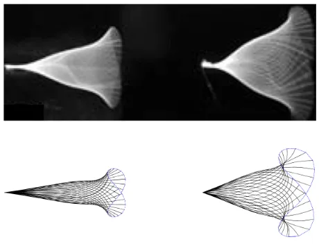
amplitudes are quite different. The amplitude of the upstream filament is found to be significantly smaller than the downstream one.

Figure 7: Beating patterns for a pair of flapping filaments in drafting configuration with a spacing ofs/L= 0.6. The flow is going from left to right. Top: Experimental visualisations obtained by Ristroph and Zhang (2008) using thin-film interferometry. Bottom: present numerical results at Re= 300.

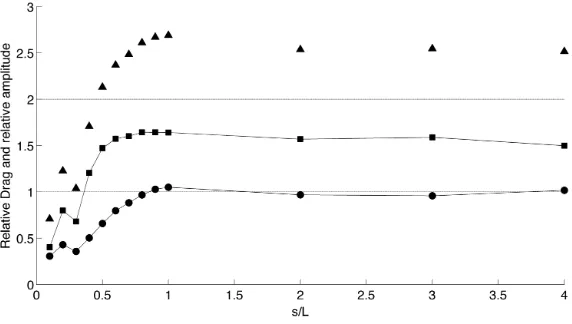
Figure 8 shows for different spacingss/L, the drag ratioD/D0 defined as

the filament drag normalised by the reference drag obtained from an isolated filament at the same Reynolds number. For a spacing less than s/L = 1, we find for the upstream filament (circles) a reduced drag compared to the reference case, while the drag stays equal to the reference case for s/L >1. Concerning the downstream filament (squares), apart from very close spac-ings (s/L < 0.3), a significant drag increase is observed compared to the reference case, up to 1.5D0. These numerical results confirm the anomalous

drafting studied experimentally by Ristroph and Zhang (2008). For the set of parameters considered, the total drag force of the system is reduced (com-pared to two isolated filaments) for all spacings s/L <0.5; and is otherwise increased. This trend is similar qualitatively to that obtained in figure 2 of Ristroph and Zhang (2008) (although we recall that the Reynolds number is different as we focus here on the relative effect with respect to the isolated case).

Figure 8: Drag ratio D/D0 as a function of the spacings/L; circles: upstream filament;

squares: downstream filament; triangles: sum of both drags.

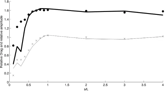
single virtually longer filament, as the gap between the filaments enables a hydrodynamic link between the filament extremities (tail and pole). This effect tends to artificially increase the bending rigidity of the virtual longer filament. As a direct consequence the amplitude of the flapping of the up-stream filament is reduced, as the amplitude of the flapping is lower near the filament pole. This assumption is confirmed by figure 9 which shows that the evolution of drag is correlated to the amplitude of flapping (measured as the maximum value of the excursion of the filament over time). Indeed a smaller upstream amplitude is associated on the figure to a smaller drag.

For large spacings (s/L > 0.5), as the upstream filament is hydrody-namically decoupled from the downstream one, its drag tends to the drag equivalent of the isolated case. However, the dowstream filament is found to have a higher drag as it experiences the perturbations induced by the wake of the upstream filament.

Figure 9: Drag ratio for upstream filament (plain line) and downstream filament (thick line) together with the amplitude of upstream filament (crosses) and downstream filament (circles), plotted as functions of the spacings/L.

reproduced.

6. Conclusions

Using a model of flexible filament incorporating its flexural rigidity, the tension (enforcing inextensibility) and the added mass, we have successfully modeled numerically the dynamics of multiple flapping filaments immersed in an uniform flow.

When considering side-by-side filaments, the wake interactions and the modal behaviour of the system have been captured correctly, in agreement with experiments (and linear stability analysis). In the present work we have restricted our attention to the influence of the filament spacing, but the influence of the added mass ∆ρ plays also a significant role (Michelin and Smith, 2009).

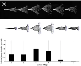
Figure 10: Six flapping filaments in an in-line configuration. Top: experiments of Ristroph and Zhang (2008). Middle: present numerical results. Bottom: Relative drag ratio for each filament.

For flapping filaments aligned with the flow, through our simulations, we have been able to confirm and partially characterise the inverted hydrody-namical drafting effect: the upstream filament is seen to experience a drag reduction compared to the downstream body. As far as drag is concerned, in agreement with the experimental observations of Ristroph and Zhang (2008), we have found that for flexible objects, the paradigm “it is better to be chased than to chase” applies, as opposite to the rigid bodies case.

Acknowledgements

The financial help of thePELskinEuropean project (FP7-TRANSPORT 334954) is greatly acknowledged.

References

Bagheri, S., Mazzino, A., Bottaro, A., 2012. Spontaneous symmetry breaking of a hinged flapping filament generates lift. Physical Review Letters 109, 154502.

Bailey, H., 2000. Motion of a hanging chain after the free end is given an initial velocity. American Journal of Physics 68, 764–767.

Bhatnagar, P., Gross, E., Krook, M., 1954. A model for collision processes in gases. i: small amplitude processes in charged and neutral one-component system. Physical Review 94, 511–525.

Domenichini, F., 2008. On the consistency of the direct forcing method in the fractional step solution of the navier-stokes equations. Journal of Com-putational Physics 227 (12), 6372–6384.

Favier, J., Revell, A., Pinelli, A., 2014. A lattice boltzmann - immersed boundary method to simulate the fluid interaction with moving and slender flexible objects. Journal of Computational Physics 261, 145–161.

Guo, Z., Zheng, C., Shi, B., 2002. Discrete lattice effects on the forcing term in the lattice boltzmann method. Physical Review E 65, 046308.

Huang, W.-X., Shin, S. J., Sung, H. J., 2007. Simulation of flexible filaments in a uniform flow by the immersed boundary method. Journal of Compu-tational Physics 226 (2), 2206 – 2228.

Malaspinas, O., 2009. Lattice boltzmann method for the simulation of vis-coelastic fluid flows. Ph.D. thesis, ´Ecole Polytechnique F´d´rale de Lau-sanne (EPFL).

Pa¨ıdoussis, M. P., 2004. Fluid-structure interactions: slender structures and axial flow, volume 2. Elsevier Academic Press.

Peskin, C. S., 2002. The immersed boundary method. Acta Numerica 11, 139.

Pinelli, A., Naqavi, I., Piomelli, U., Favier, J., 2010. Immersed-boundary methods for general finite-difference and finite-volume navier-stokes solvers. Journal of Computational Physics 229 (24), 9073 – 9091.

Qian, Y., D’Humieres, D., Lallemand, P., 1992. Lattice bgk models for navier–stokes equation. Europhysics Letters 17 (6), 479–484.

Ristroph, L., Zhang, J., 2008. Anomalous Hydrodynamic Drafting of Inter-acting Flapping Flags. Physical Review Letters 101 (19), 194502–4.

Schouweiler, L., Eloy, C., 2009. Coupled flutter of parallel plates. Physics of fluids 21, 081703.

Shelley, M. J., Zhang, J., 2011. Flapping and bending bodies interacting with fluid flows. Annual Review of Fluid Mechanics 43 (1), 449–465.

Succi, S., 2001. The lattice Boltzmann equation. Oxford university press New York.

Tian, F.-B., Luo, H., Zhu, L., Lu, X.-Y., 2011. Coupling modes of three filaments in side-by-side arrangement. Physics of Fluids 23 (11), 111903.

Uhlmann, M., 2005. An immersed boundary method with direct forcing for the simulation of particulate flows. Journal of Computational Physics 209 (2), 448476.

Zhang, J., Childress, S., Libchaber, A., Shelley, M., 2000. Flexible fila-ments in a flowing soap film as a model for one-dimensional flags in a two-dimensional wind. Nature 408, 835–839.

Zhu, L., Peskin, C. S., 2000. Interaction of two flapping filaments in a flowing soap film. Physics of fluids 15, 1954–1960.