Control Design of a PFC with Harmonic Mitigation
Function for Small Hybrid AC/DC Buildings
Rafael Pe˜na-Alzola,
Member, IEEE,
Marco Andr´es Bianchi,
Student Member, IEEE,
and Martin Ordonez,
Member, IEEE
Abstract—Unprecedented expansion of native DC powered equipment (LEDs, computers and consumer electronics) has increased commercial and residential DC electricity usage over the past decade. Thus, it is foreseeable that hybrid AC/DC buildings featuring both AC and DC infrastructures will coexist. A hybrid AC/DC building will involve an efficient centralized rectifier that supplies all the DC loads, while legacy AC loads will remain connected to the existing AC infrastructure. This paper explores the opportunity of harmonic mitigation at distribution level in small hybrid AC/DC building by using a centralized power factor corrector (PFC) with large bandwidth. The current reference generator for the harmonic mitigation function (HMF) is explained along with power considerations. The PFC uses a proportional resonant (PR) controller, instead of a PI controller, without requiring additional sensors in the rectifier. A computa-tionally inexpensive implementation of the PLL is also proposed along with considerations on parameter selection. The proposals provide all the steps for the straightforward control design of the PFC+HMF with fast calculations. The HMF requires only software modifications in the PFC and one sensor to measure the non-linear load. Simulation and experiments validate the proposed procedures.
Index Terms—Power factor correctors, proportional resonant controller, semibridgeless PFC, boost PFC, harmonics
I. INTRODUCTION
T
HE increase in DC electricity usage is putting even more pressure on a century-old AC power infrastructure. In the present AC building as the one depicted in Fig. 1, DC loads such as LED lighting, compact fluorescent lamps, electric vehicles (EVs), and computers require individual AC/DC rectifiers that result in increased cost and lower efficiency. As more and more loads are native DC loads, a transition to DC buildings and houses is expected [1], [2]. In DC buildings and houses, an efficient centralized rectifier supplies all the DC loads. The advantages of replacing the unnecessary individual rectifiers with a centralized rectification include: higher effi-ciency, lower costs, higher reliability, smaller footprint, and better power quality.It is foreseeable a long period of hybrid AC/DC buildings in which the AC and DC infrastructures coexist and complement each other [1]. This situation is depicted in Fig. 2, where the DC loads are connected directly to the new DC infrastructure and legacy AC loads are connected to the already existing infrastructure. As legacy AC loads normally comply with
R. Pe˜na-Alzola, M. A. Bianchi, and M. Ordonez are with the depart-ment of Electrical and Computer Engineering, The University of British Columbia. 2332 Main Mall, Vancouver V6T 1Z4, BC Canada. E-mail: [email protected]; [email protected]; [email protected]).
M Diode PFC Diode PFC i PCC t i PI Individual Rectification Individual Rectification
Regular PI controlled PFC Regular PI controlled PFC
Flyback Flyback
LED
LED CFLCFL
Buck-Boost Buck-Boost EV Battery EV Battery Electronic Ballast Electronic Ballast Diode PFC Diode PFC Diode PFC Diode PFC 3 2 1
NATIVE DC LOADS NATIVE DC LOADS 1 2 LINEAR LOADS LINEAR LOADS Consumer Electronics Consumer Electronics Flyback Flyback Servers Servers LLC LLC Full Bridge Full Bridge VSD HVAC VSD HVAC
NATIVE DC LOADS NATIVE DC LOADS
Diode PFC Diode PFC Diode PFC Diode PFC 2 2
THD > 5% | PF < 1
[image:1.612.313.563.186.349.2]3
Fig. 1. Typical issues in traditional AC building including many native DC loads: low power quality (1) due to the presence of non-linear loads; lower total rectification efficiency due to individual rectification (2); PFC rectifiers mainly based on PI controller (3) that have limited sinusoidal tracking capabilities.
THD < 5% | PF 1
i PCC t i NL t ~ − t i PFC Centralized Rectification Centralized Rectification
PR controlled PFC with Harmonic Mitigation (HM) PR controlled PFC with Harmonic Mitigation (HM)
PCC Isolated Conv. LEGACY LOADS LEGACY LOADS LINEAR LOADS LINEAR LOADS 1 2 3
3 LEDLED
NATIVE DC LOADS NATIVE DC LOADS HVAC
HVAC EV
EV ServersServers
Consumer Electronics Consumer Electronics 1 CENTRALIZED RECTIFICATION CENTRALIZED RECTIFICATION PCF+HM Rectifier PCF+HM Rectifier
2 PR i
Fig. 2. Advantages of hybrid AC/DC building including the proposed PFC with harmonic mitigation function (HMF): 1) power quality of the building is increased through the HMF; 2) the centralized rectification scheme has the advantage of increasing the total conversion efficiency and reducing the overall cost; 3) the Proportional Resonant (PR) controller can track sinusoidal signals accurately.
[image:1.612.314.563.420.562.2]means to compensate the distribution system harmonics are needed [3]. Unlike the industrial loads in a medium voltage network, the non-linear loads in the low-voltage distribution are highly distributed [3]. Lump harmonic compensation using passive filters or centralized active power filters at a few locations is difficult [5] and distributed compensation could be a better solution [6], [7]. Power converters of renewable energy systems (wind and solar) can be used for harmonic compensation [3], [4], using the available volt-ampere when not operating at full capacity. However, this solution is only possible where the renewable resource is available.
In North America, center-tapped transformers convert one distribution phase to a split-phase 120/240 V in small buildings (residential and light commercial) [8], [9]. The centralized rectifier in Fig. 2 comprises a single-phase PFCs followed by an isolated DC/DC converter. Single-phase PFCs rectify the input AC voltage with sinusoidal AC currents and unity power factor. The most well-known topologies for single phase PFCs are boost, bridgeless and semi-bridgeless [10], [11]. An elevated switching frequency (tens to hundreds kHz) enables filter size to be reduced and power density to be increased [12], [13], while improving the dynamic response of the converter. The isolated DC/DC stage (e.g. LLC resonant converter or phase shifted ZVS topology) [11] blocks the common mode voltage and provides the final DC output voltage. Despite the potential of single-phase PFCs to improve power quality, there are only a few references exploring the possibility of the single-phase PFC dealing with harmonics [14]–[16]. This is because the Harmonic Mitigation Function (HMF) requires active power transfer to the DC load as will be discussed in this paper. In [14], a technique was used for telecom parallel rectifiers combining PFCs with diode bridges. The PFCs compensate the harmonics generated by the diode bridges while supplying the load.
Considering the progressive and general transition to hy-brid AC/DC buildings and the large bandwidth available in the centralized PFC, this paper explores the opportunity for harmonic mitigation in the distribution system. This useful function, conceptually depicted in Fig. 2, was not considered in any of the previous works on PFC described above. The paper presents the control design for a PFC with harmonic mitigation function (PFC+HMF). The proposed control design is based on three main subsystems: current reference generator for the HMF, PR controller for the current reference tracking, and efficient PLL implementation.
The proposed current reference generator for the HMF obtains information from measuring the non-linear current and determines the PFC current reference needed for mitigating the harmonics in the system. The operation is explained along with its limitations and power considerations.
The control loop for the proposed PFC+HMF uses a propor-tional resonant (PR) controller, which is discussed in detail, to effectively track the proposed HMF. PFCs usually employ PI controllers [17] that produce a phase delay when tracking a sinusoidal reference [18]. Controlling the grid current directly [19], [20] by using a proportional resonant controller (PR)
enables tight tracking of sinusoidal signals at the resonance frequency with no phase error [21]. Parallel PR controllers [22]–[24] allow tracking references at multiple frequencies at the expense of increased computations. Considerations on the implementation of the PR controller were explained in [21], [24], [25], and tuning procedures in [18], [26], [27]. The proposed PFC+HMF uses a PR controller what guarantees fast and accurate tracking of the current reference without requiring additional sensors in the PFC. Considerations on discretization and parameter tuning of the PR controller are provided.
One more important element addressed in this paper is the PLL implementation for the PFC+HMF. Single-phase PFCs requires a PLL for synchronization with the voltage at the point of common coupling (PCC). PLLs based on adaptive filtering are now widely used; SOGI-PLL [28], [29] and the SOGI-FLL [28]. This paper proposes and computationally inexpensive implementation of the SOGI-PLL and parameter tuning considerations are also provided.
The elevated switching frequency puts high requirements for the DSP and efficient control algorithms should be proposed. The proposals in the paper provide all the steps for the straightforward control design of the PFC+HMF with fast calculations. The proposed HMF scheme allows moderate non-linear loads to be compensated at low cost, with only software modification and one current sensor for the non-linear load.
This paper is organized as follows: the current reference generator for the HMF in the hybrid AC/DC building is explained in Section II. Section III describes the utilization of PR controllers in PFC rectifiers. Section IV explains considerations on the implementation of the PR controller. Section V describes the efficient implementation of SOGI-PLL. Simulation and experimental results are shown in Section VI and VII respectively. Finally, Section VIII concludes the paper.
II. HARMONICMITIGATION INSMALLHYBRIDAC/DC BUILDINGS USINGPFC
The proposed HMF in the small hybrid AC/DC building is constrained by the unidirectionality of the diodes in the PFC rectifier. Hence, the PFC current must have the same sign as the voltage.
A. Current reference generator for the harmonic mitigation function
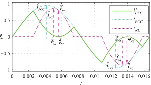
In order to obtain the current reference for the HMFi∗P F C, the non-linear load currentiN Lis sensed. As the PFC rectifier is unidirectional, the necessary PFC current reference i∗P F C
0 0.002 0.004 0.006 0.008 0.01 0.012 0.014 0.016 −1
−0.5 0 0.5 1
t
pu
i PFC i
PCC i
NL *
I^NL
^
φ^
^
φ NL
^ NL
INL
^
IPCC I NL
φ NL
IPCC INL
[image:3.612.53.300.69.208.2]NL φ
Fig. 3. Currents resulting from current reference generator for the HMF.
voltage. The PFC current reference needed to absorb the non-linear current is:
i∗P F C(t) = ˆIP CC·sin(ωnt)−iN L(t) (1)
with
ˆ
IP CC = ˘IN L/sin( ˘φN L) = max t∈Tn/2
(iN L/sin(φN L)) (2)
Thus, IˆP CC corresponds to the largest value of the ratio
iN L/sin(φN L) for each semi-cycle, see Fig. 3. This corre-sponds to the tangent point, with amplitude I˘N L and phase
˘
φN L. The PCC current will be sinusoidal with amplitude equal toIˆP CC in phase with the PCC voltagevn=
√
2Vnsin(ωnt), which is assumed to be perfectly sinusoidal for the sake of simplicity. It can be seen in Fig. 3 thati∗P F C(t)is positive for the positive PCC voltage (proportional toiP CC), fulfilling the condition of unidirectionality in the PFC diodes.
B. Harmonic Composition Analysis
For the harmonic composition analysis it is assumed that the tangent point I˘N L is close to the maximum point IˆN L so
ˆ
IP CC ≈IˆN L/sin( ˆφN L), see Fig. 3. The harmonic composi-tion of the non-linear current is as follows:
iN L(t) = ∞ X
i=1
√
2IN Li·sin(iωnt−φN Li)
=√2IN L1·cos(φN L1)·sin(ωnt)
−√2IN L1·sin(φN L1)·cos(ωnt)
+ ∞ X
i=2
√
2IN Li·sin(iωnt−φN Li)
(3)
The first term of (3), fundamental current in phase with the PCC voltage, corresponds to the active power PN L =
VnIN L1cos(φN L1). The second term of (3), fundamental current in quadrature with the PCC voltage, corresponds to the reactive power QN L=−VnIN L1sin(φN L1). Finally, the last term of (3) corresponds to the harmonic current iN Lh.
Substituting (3) in (1), the harmonic composition of PFC rectifier current reference is as follows:
i∗P F C =IˆP CC−
√
2IN L1·cos(φN L1)
| √ {z }
2I∗ P F C1
·sin(ωnt)
+√2IN L1sin(φN L1)·cos(ωnt)
−
∞ X
i=2
√
2IN Li·sin(iωnt−φN Li) (4)
The second term of (4), fundamental PFC current in quadra-ture with the PCC voltage, is to compensate the reactive power produced by the non-linear load (QN L) so the reactive power produced by the PFC isQ∗P F C =−QN L. The third term of (4) cancels the harmonic currents produced by the non-linear load (iN Lh) so that the harmonic current produced by the PFC is
i∗P F Ch=−iN Lh. These two cancellation terms are the usual ones in single phase active filters. However, the PFC rectifier, because of its unidirectionality, must consume active power
PP F C1 = VnIP F C∗ 1 in order to perform the compensation. This requirement corresponds to the first term of (4), defined as√2IP F C∗ 1, which is fundamental PFC current in phase with the PCC voltage. Substituting the definitions of the crest factor (CF = Ipeak/Irms) and the total THD of the load current, the required fundamental PFC current is:
IP F C∗ 1= ˆ
IP CC
√
2 −IN L1·cos(φN L1) =
=IN L1
CFiN L q
1 +T HD2 iN L
√
2·sin( ˆφN L) −cos(φN L1)
(5)
According to (5), the required current IP F C∗ 1 increases with the fundamental current, the harmonic content (CF and
T HD), and finally the displacement power factor (DP F = cos(φN L1)) of the non-linear load. It is clear that this scheme only makes sense when the required active power PP F C1 is useful. The active power consumed by the PFC rectifier is determined by the closed loop control of the DC-link capacitor voltage. If the power requested by the PFC rectifier load is lower than the minimum power PP F C1, the compensation scheme is not possible.
could be developed.
The proposed current reference generator for the HMF is fully consistent with the harmonic content analysis explained in [14], which uses the harmonic reference generator from [30]. This analysis considers symmetrical non-linear loads (φˆN L ≈90◦−φN L1), which allows further simplification in (5) to obtain the value of the fundamental PFC current.
C. Stability considerations
It can be seen in (4) that the current reference to the PFC corresponds to the reactive power and all the harmonics of the non-linear load plus a fundamental component. The current reference generator for the HMF is a feedforward procedure that corresponds to the load detection method widely employed in shunt active power filters [31], [32]. This procedure is appropriate when the non-linear loads behave as current sources where the parallel inductance is much larger than the grid inductance [33]. In the shunt active power filter, the fundamental component is needed for compensating the converter losses. In the PFC, the fundamental component is required because of the PFC unidirectionality. Stability consideration for the load detection algorithm can be found in [33], [34].
Harmonic compensation in closed loop [35], [36] uses the grid current iP CC as control variable. The slow DC-link voltage control generates the sinusoidal reference irefP CC. The compensation is slow, but it is accurate [35] and has good sta-bility characteristics [36]. In addition, the DC-link capacitors must be large enough to cope with the power variations in the non-linear load [36]. PFCs use electrolytic capacitors for DC-link and, thus, this requirement is not constraining. Fig. 6, explained later on, shows the block diagram for this approach in closed loop.
III. USE OF PROPORTIONAL RESONANT CONTROLLERS IN
PFCRECTIFIERS
The PFC+HMF needs to be able to track the reference signal without phase error. This is achieved by the use of a PR controller, which resonant part allows the accurate tracking of the fundamental component of the current. This section describes the principle of operation of using a PR controller with the most well-known PFC topologies and the considerations that should be taken into account.
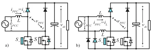
A. Boost PFC topology
The boost PFC topology is shown in Fig. 4. The current reference of the boost PFC rectifier is a signal proportional to the absolute value of the PCC voltage. This signal is obtained from the PLL synchronized to the grid PCC voltage. From the control perspective, the boost PFC can be seen as a regular boost DC/DC converter with variable input voltage and variable current reference. The input signal waveforms are the absolute value of sinusoidal functions. Fig. 4 highlights the semiconductors involved during the positive half of PCC
L R
C v
PCC
i L
v PFC
v dc
S
[image:4.612.313.564.55.162.2]i PFC
Fig. 4. Power factor correctors (PFC): boost topology
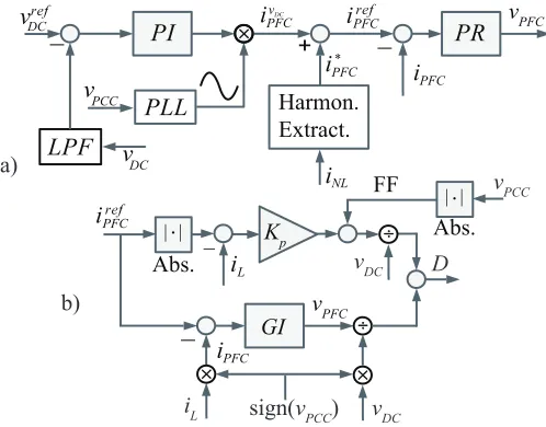
vPFC PFC
PFC PCC
NL DC
DC
PFC * PFC
vDC
Harmon. Extract.
a)
Kp Abs.
PFC
L
vPFC
PFC
sign(vPCC)
iL
÷
D
vDC
GI
| |
÷
vPCC
vDC
| | Abs.
b)
FF .
.
Fig. 5. a) Overall block diagram of the PFC with HMF. b) Detailed view of the PR implementation
voltage. In order to use a PR controller, the sinusoidal output current is directly controlled in the closed loop. For this purpose, the following transformation is used to obtain the sinusoidal output current iP F C inferred from the inductor current and the PCC voltage:
iP F C =iL·sign(vP CC) (6)
whereiLis the inductor current,vP CCis the grid PCC voltage, and sign(·) is the sign function. The current reference is a sinusoidal waveform synchronized to the PCC voltage and limited to be:
0≤irefP F C ≤IP F Cmax forvP CC≥0
−IP F Cmax ≤i ref
P F C<0 forvP CC<0
(7)
whereImax
P F C is the PFC converter current limit. These limits force the current to be positive when the PCC voltage is positive and vice versa. The output of the PFC boost converter
vP F C is related to the boostDcycle duty cycle according to:
vP F C =vDC·Dcycle·sign(vP CC) (8)
with vDC the DC-link voltage. This means that the boost PFC provides positive voltagevP F C for positive PCC voltage
[image:4.612.312.561.198.393.2]v
PFC PCC
PCC PCC
DC DC
[image:5.612.310.565.53.140.2]PFC
Fig. 6. Closed-loop approach for the HMF.
Unlike previous approaches [19], [20], the proposed trans-formations require no additional sensors to infer the value of iP F C. However, there is uncertainty in the current sign around the zero crossing due to the non-linear behavior of the real diodes. It is known that the low voltage around the zero crossing is a source of distortion in the PFC current depending on the PCC voltage, current and inductance [37], [38]. In order to reduce the effect of the misinterpretation in the current sign at the zero crossing, the proportional gain of the PR controller can be applied without the transformations (6)-(8) and with the current reference being a rectified sinusoidal as shown in Fig. 5b. In this form, the fast proportional action can correct potential errors caused by uncertainties. Comparing to the PI controller, the PR controller requires only one additional integrator as it can be seen in Fig. 8 (explained later on). In addition, the logic for selecting the proper voltage cycle (6)-(8) comprises only sign multiplications as it can be seen in Fig. 5b.
As depicted in Fig. 6, the closed loop approach of the controller employs iP CC as the control variable. SinceiP CC is a measured sinusoidal variable transformation (6) is not necessary. In addition, it is difficult to protect the PFC con-verter as the current is not indirectly controlled. The current reference irefP CC can be saturated to ±Imax
P F C + iN L with
iN L = iP CC −iP F C calculated from the measured iP CC and (6).
When the PR controller is included in the PFC rectifier control, the overall block diagram, shown in Fig. 5a, is the same as that of a regular bidirectional grid-tie H-bridge [18]. This consists of two nested loops; the inner and faster for the PFC current iP F C and the outer and slower for the DC-link voltagevDC. In addition, the PFC rectifier must also produce the current reference for the HMF i∗P F C explained in section II. Hence, the total current reference for the PR controller
irefP F C is the sum of the DC-link controller output ivDCP F C and the HMF current i∗P F C as shown in Fig. 5a. The alternating power at twice the fundamental frequency and the harmonic power will reflect in the DC-link capacitor of the PFC rectifier as DC-voltage ripple. The DC-voltage should be low-pass filtered with a DC-voltage control bandwidth bellow twice the line frequency so as not to interference with the current loop. The HMF will only work when the DC-link voltage is properly regulated. For high and low values of DC-voltage, the compensation current reference should be progressively reduced.
L iPFC=iL
vPCC v
dc v
PFC
S+ S
-L
i PFC=iL
vPCC v
dc v
PFC
S+ S
-a) b)
[image:5.612.50.316.57.140.2]L
Fig. 7. Power factor correctors (PFC): a) bridgeless PFC and b) semi-bridgeless PFC.
B. Bridgeless and semi-bridgeless PFCs
Compared to the previous PFC boost topology, PFC topolo-gies shown in Fig. 7, eliminates one diode from the line-current path reducing the conduction losses [10]. Because of the increasing pressure for better efficiencies, this bridgeless PFC topology is expected to be present in the AC/DC hybrid buildings. The topologies for the bridgeless PFC and the semi-bridgeless PFC [11] are shown in Fig. 7a and Fig. 7b respectively. Fig. 7a highlights the semiconductors involved during the positive semi-period of the PCC voltage in the bridgeless topology. The bridgeless topology can be viewed as a full bridge active rectifier, in which the upper switches have been removed because they are redundant when only unidirectional power flow is required. The current circulating through the converter inductor is the same as the grid current and a PR controller can be used to control it.
Fig. 7b highlights the semiconductors involved during the positive semi-cycle of the PCC voltage in the semi-bridgeless PFC. Two slow diodes have been added to clamp the output ground to the AC source terminals, and an additional inductor is needed for each half of the PCC voltage waveform. The resulting topology consists of two boost DC/DC converters, working alternatively for the positive and negative semi-cycle of the grid voltage waveform. From the control perspective, the alternating boost DC/DC converters of the semi-bridgeless PFC rectifier also have a variable input voltage, and the current reference is the absolute value of a sinusoidal waveform. In order to use PR controllers with the semi-bridgeless PFC, the previous transformations and limitations (6)-(8) must be applied to reconstruct the grid current from the inductor currents and the PCC voltage.
IV. IMPLEMENTATION OF THEPRCONTROLLER
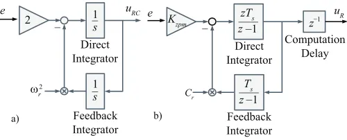
This section explains considerations on the discretization and proper tuning of the PR controller. The PR controller comprises two parts: a proportional gain and a generalized integrator (GI):
P R(s) =Kp+GI(s) =Kp+Kr 2s s2+ω2
r
(9)
a) b)
2
e 1
s
1
s
uRC e Kzpm
ω
r
2
uR
z
z
1
1
zTs
Ts
z1
Direct Integrator
Feedback Integrator
Direct Integrator
Feedback Integrator
Computation Delay
Cr
Fig. 8. a) Implementation of the resonant controllers using two integrators, b) proposed discretization.
A. Discretization
This section explains considerations on discretization to prevent mismatch in the resonance frequency between the continuous and discrete implementation of the PR controller. The GI part of the PR is usually implemented using two integrators, as shown in Fig. 8a. The Bilinear method with pre-warping (Tustin method) allows the characteristics of (9) at the resonant frequency to be preserved [39]. However, the use of the zero matching method allows one additional degree of freedom in the discretized equivalent that results in [25]:
GI(z) =Kzpm
2(1−z−1)z−1 1−2z−1cos(ω
rTs) +z−2
(10)
The Fig. 8b shows the discrete implementation of the GI. In order to avoid an algebraic loop, [21] suggest to use forward Euler for the direct integrator and backward Euler for the feedback integrator. However, in the implementation of Fig. 8b uses backward Euler for the direct integrator, forward Euler for the feedback integrator, and incorporates the computation unit delay explicitly. This results in the same transfer function, and it is more convenient conceptually for automatic code generation from the simulation software. The code generation tool usually generates code for the control blocks and the computation delay results from the execution. The transfer function from direct discretization of both integrators is:
P R(z) =Kp+Kr
2Ts(1−z−1)z−1 1 +z−1(C
rTs2−2) +z−2
(11)
The resonant frequency of the PR controllers is taken from the grid frequency calculated in the PLL [24], [40] to preserve the infinite gain at the resonant frequency. Considering that the grid frequency is always close to the rated grid frequency
ωn [18], it is proposed to use Taylor series around ωn for cosωrTs in (10). This results in more accuracy for the same computational effort than using McLaurin series as was done in [24], [40]. Thus, the factorCr in Fig. 8 is:
Cr= 2
T2 s
− 2
T2 s
cos(Tsωn) + 2
Ts
sin(Tsωn)(ωr−ωn)
+ cos(Tsωn)(ωr−ωn)2+... (12)
The gain Kzpm is selected to have the same value in the discrete and continuous domain for a critical frequency, usually DC s =ωj = 0 [39]. In order to preserve the high
gain characteristic around ωr, the gain Kzpm is selected to have the same bandwidth (-3 dB) in the discrete equivalent as in the continuous system. The gain of theGI(s)is -3 dB for the following frequency:
ω−3dB= s
ω2
n+ 4±4 r
ω2 n
2 + 1 (13)
Therefore, GI(z) at z = ejω3dBTs should have the same
gain of -3 dB. Using the bilinear approximation es ≈ (1 +
s/2)/(1−s/2) and neglecting small second order terms, the gainKzpmis selected as follows:
Kzpm≈
ωnTs q
ω2 n+
√
2ωn
(14)
With these considerations the PR controller can be properly tuned to the grid frequency allowing the proper tracking of the fundamental component.
B. Parameter tuning
The HMF requires the proper tuning of the PR controller to attain a proper bandwidth for tracking the harmonic com-ponents. The proportional gain Kp of the PR controller de-termines the control bandwidth [21]. The GI has an effect only in the near range of the fundamental frequency [21], its effect is neglected for the rest of the frequency spectrum and only the proportional gain Kp is considered. The PWM and computation delays and the inductor resistance are also neglected and the plant is only Gp(s) = 1/Ls with L the connection equivalent inductance. The closed loop system is as follows:
Gcl=
KpGp(s) 1 +KpGp(s)
= L 1 Kps+ 1
(15)
The bandwidth is ωbw = 2πfbw = Kp/L and must be selected well bellow the switching frequency. The proportional gainKp for a bandwidthfbw≈fsw/10is:
Kp=
2πLfsw
10 (16)
This value is consistent with the suggested value of PI con-trollers in [41]. Considering the elevated switching frequencies (tens to hundreds kHz) the achieved bandwidth (kHz to tens of kHz) allows the proper tracking of the harmonic components in the HMF for the small hybrid AC/DC building.
In the following discussion, the integration time Tr =
Kp/Krfor the PR controller is defined as the ratio between the proportional and resonant gains. Assuming the same previous simplification, the transfer function relating the reference and the error is:
Ge(s) = e(s)
yref(s)
= 1
1 +P RLs(s) (17)
[image:6.612.49.299.55.156.2]eapprox(s) = 5Ts
πω2 r
s2
5Ts πω2 r
s3+ 1 ω2
r
s2+ 2 N Tsω2r
+5Ts π
s+ 1 (18)
For the following derivations, the term s3 is neglected for elevated switching frequencies and 2/(N Tsω2r) >> 5Ts/π. The inverse Laplace transformation of (18) is a decaying exponential function multiplying sinusoidal functions. The decaying time constant and the initial value are respectively:
τ =Tr (19a)
eapprox(t= 0) =− 10
π Ts
Tr
(19b)
A conservative estimation of the settling time can be ob-tained by approximating the sinusoidal functions of the inverse Laplace transform of (18) to the unity. Therefore, as a simple decaying exponential with time constant with initial value (19),
eapprox(s) =− 10Ts
π
1
Trs+ 1
(20)
And the settling time (2%) is approximately:
ts2%=Trln 500T
s
πTr
(21)
The settling time increases for increasing values of Tr, the estimation (21) increases for increasing values of Tr until it reaches a maximum. Therefore, the estimation (21) is valid for values of Tr<500Tse−1/π≈60Ts, less than this maximum where the previous approximations do not hold anymore.
C. Stability
In the previous analysis, the PWM and computation delays and the inductor resistance were neglected. However, these parameters influence stability and should be considered. As the bandwidth was selected a decade lower than the switching frequency, the analysis can be safely done in the continuous domain. The transfer functions for the inductor, considering the resistance, and for the PWM and computation delays are respectively:
GRL(s) = 1
Ls+R (22a)
Gdelay(s) = 1 1.5Tss+R
(22b)
The PWM and computation delays, with duration a half and a full switching period respectively, are approximated as a first order system [41]. The open loop transfer function isGcl(s) =
P R(s)Gdelay(s)GRL(s). The conditions for stability for the previous proportional gain (16) are obtained by applying the Routh-Hurwitz criterion to the denominator of the closed loop transfer function:
Tr>
6L2Tsπ 2L2π+ (10 + 3π)LRT
s+ 15R2Ts2
(23a)
Tr>
6L2T sπ
2L2π+ (10 + 3π)LRTs+ 15R2Ts2−90LRT 3 sf
2 nπ
2
−60L2fn2π2Ts2 (23b)
It is clear that condition (23b) includes condition (23a) and both are satisfied for Tr > 3Ts. Taking into account this finding and (21), a proper value is:
Tr= 15Ts (24)
This is ten times the time constant of Gdelay(s), as was proposed in [41] for PI controllers.
V. SOGI-PLLIMPLEMENTATION
The PLL enables the generation of the current reference signal and calculates the gri frequency what makes it an elemental subsystem of the PFC-HMF controller. This section explains the operation of the employed SOGI-PLL along with two algorithms that optimize the execution of the PLL. In this paper, the SOGI-PLL proposed in [29] and shown in Fig. 9 will be used for PCC voltage synchronization.
The SOGI-PLL consists of passing the PCC voltage through a bandpass and a low-pass filter. The filter is usually one SOGI section that enables the construction of a second order low-pass and a bandlow-pass filter. The gain K is usually selected
ζ = 0.707 to result in a Butteworth filter. In this paper, it is proposed that K be selected to result in a Bessel filter,
ζ = 0.866, in order to better preserve the voltage waveform phase, as the Bessel filter has maximally linear phase response [42]. If the PCC voltage is very polluted, in [43] it is proposed to use the multiple SOGI sections to increase the harmonic attenuation. In such cases, it is proposed that the coefficients of thenSOGI sections will match a higher order (2n) Bessel filter in factored form, which can be found in [42].
The outputs of the bandpass and a low-pass filters result in two orthogonal componentsαandβ, which are fed into a regular dq-PLL that calculates the grid frequency and phase (see Fig. 9). The procedure requires the application of a coordinate transformation given by,
vTdq=R(θi)vTαβ=
v0d qvq0
=
cosθi sinθi
−sinθi cosθi
v0 qv0
(25)
Bandpass and Lowpass Bessel Filter PCC
Fig. 9. Block diagram of the SOGI-PLL used for grid synchronization.
A. CORDIC algorithm
The CORDIC algorithm expresses the coordinate transfor-mation matrix [44] in the following form:
R(θi) = 1
√
1 + tan2θ
1 tanθi
−tanθi 1
(26)
In vectoring mode, the CORDIC algorithm selects angles
γi = arctan(2i) to rotate the vector v0, qv0 to x-axis. The operations tan(γi) = 2i can be done with simple shifts in fixed-point hardware, see details in [45].
Hence, the CORDIC algorithm enables the calculation of the angle error arctan(qv0/v0) in the PLL and the PCC voltage module|v0|with low computational resources. The angle error is used in the PI controllers of the PLL, as it is shown in Fig. 9. The PCC voltage module |v0|is necessary for the DC-link voltage control, in order to enable the proper working of the PFC rectifier at different grid voltage levels.
In addition, the module|v0|value can be used to compensate the reactive power produced by the x-cap of the EMI filter. The usual remedy for this problem consists of delaying the current reference [46], and this problem worsens for light loads. Assuming that the voltage across the x-cap is approx-imately the PCC voltage, the consumed reactive power is
Qx = v2P CCCxωn with Cx the total capacitance of the x-caps. Therefore, a current component in phase with qv0 and of module|v0|Cxωn, both magnitudes estimated from the PLL, should be introduced to compensate the x-cap reactive power.
B. Iterative implementation
The phase angle is the output of an integrator fed by the PI controller output plus the feed-forward of the rated frequency, as shown in Fig. 9. Assuming Euler forward discretization for the integrator:
θi+1=θi+ (ωn+uP In)Ts (27)
whereωn refers to the rated frequency, which is fed-forward for fastest settling time, and uP In is the PI controller out-put, which is limited for antiwindup. Hence, the coordinate transformation is:
TABLE I
PARAMETERS FOR THE SIMULATIONS AND EXPERIMENTS.
Parameter Symbol Value Rated AC voltage Vn 120 V Rated current In 2.8 A Rated frequency fn 60 Hz Inductor inductance L 0.550 mH Inductor resistance R 7 Ω DC link voltage vDC 200 V DC link capacitor CDC 560µF Sampling frequency fs 60 kHz PWM frequency fsw 60 kHz
R(θi+1) =R(θi)R(ωnTs)R(uP InTs) (28)
The matrixR(ωnTs)is fixed and can be pre-calculated. By limiting the output uP In < ±0.75/Ts, the coordinate trans-formation matrix can be approximated using Taylor series:
R(θ) = "
1−θ2
2 θ
−θ 1−θ2
2 #
(29)
with an accuracy less than 10% using far fewer operations. The limitation in the outputuP Inresults in a slower response. Higher limits for uP In can be selected by using more Taylor terms in (29) for faster response at the expense of more computations. After calculating thedq-components of the PCC voltage, the angle error must be calculated by using the arctangent function that can be approximated as a division atan2(vq, vd)≈vq/vd.
The double integrator (system type II) of the PLL allows the ramp angle reference to be followed without steady state error. The proportional gain and integration time are proposed to be tuned to get the optimum coefficients in the closed loop transfer function based on the ITAE criterion (damping factor
ζ= 1.6 [47]) for a ramp input:
Kp= 5.76fbw ≈ 43.2
ts
(30a)
Ti= 1.76
fbw
≈ ts
4.2 (30b)
withtsthe settling time (1%), usually100 msfor this type of PLL [18], andfbw the bandwidth (-3 dB).
VI. SIMULATION RESULTS
Table I shows the parameters of PFC+HMF (boost topology) used in the simulations. The control blocks were modeled using Matlab/Simulink and the semiconductor devices using PLECS.
0 0.005 0.01 0.015 0.02 0.025 -1
-0.5 0 0.5 1
t pu
Current reference PR controller PI controller
b) a)
0 2 4 6 8 10 12 14 16
Harmonic Order %
0 0.5 1.2 99.8 100
PR controller
[image:9.612.312.564.56.192.2]PI controller
Fig. 10. Comparison between a) the cosine-step responses and b) low-frequency spectra of PR and PI controllers (simulation results) in the boost PFC current control. The PR controllers results in faster response, power factor closer to unity, and lower harmonic content.
the PR controller, the transformations (6)-(8) are used to infer the grid current and the selected anti-windup mechanism is conditional-integration. Both controllers have the same pro-portional gain (16) with approximately the same bandwidth
fbw ≈ fsw/10. The integration time (24) is the same for both controllers, ten times the smallest time constant of the control plant τ = 1.5Ts [41], as explained in Subsection IV-B. It can be seen that the response when using the PR controller is faster. The PR controller allow to accurately track the sinusoidal reference with no delay resulting in better power factor. The small variations for the PR controller, before the cosine step input, are due to the proportional action at the zero crossing. Finally, the use of the PR controller results in less zero-crossing distortion as shown Fig. 10a, and this results in lower harmonic content as shown in Fig. 10b.
Fig. 11 shows the gain at ω−3dB (13) for the continuous case and the discrete cases at different sampling frequencies
fs. The discrete cases are the proposed zero-pole mapping discretization with gainKzpm according to (14) and the usual Tustin with pre-warping Kzpm = sin(Tsωn)/ωn. For low switching frequencies, fs/fn < 7, the proposed gain Kzpm results in overly large values and the Tustin gain in low values (and so narrower bandwidth). For these cases the gain Kzpm should be calculated numerically in order to preserve the same bandwidth in the continuous and discrete cases. For moderate sampling frequencies, 7 < fs/fn < 20, the proposed gain
Kzpm guarantees a higher bandwidth in the discrete model. For high sampling frequencies, fs/fn > 20, the differences
5 10 15 20 25 30
−4 −2 0 2
G
ai
n (dB
)
fs/fn
[image:9.612.51.302.58.332.2]Continuous Proposed Tustin
Fig. 11. Gain of the PR controller for the continuous case, the proposed zero pole matching, and Tustin with pre-warping. For moderate sampling frequencies,7< fs/fn<20, the proposed gainKzpmguarantees a higher
bandwidth in the discrete model.
0 1 2 3 4 5 6 7
−0.5 0 0.5 1
t (10-4 s)
pu
Eq. (18) Eq. (18) simpl. Exact Eq. (20)
Fig. 12. Tracking error versus time of the different approximation for the cosine step input in the PR controller. Eq. (20) leads to a very conservative estimation for the settling time (21) that is simple to calculate and does not require simulations.
between the three cases are indistinguishable as expected.
Fig. 12 compares the tracking error of the cosine step input when using a PR controller for the exact model, the approx-imation according to (18), the approxapprox-imation (18) neglecting the third order term, and finally the approximation according to (20). The settling times (2%) for the different cases are 39 ms, 38 ms, 35 ms and 70 ms respectively. Hence, the model according to (18) is very accurate, even when neglecting the third order term. Because of the simplifications, the model according to (20) leads to a very conservative estimation (21), as stated in its derivation in Subsection IV-B, which is simple to calculate and does not require simulations.
Fig. 13 compares phase tracking of SOGI-PLL with and without the simplifications proposed in Subsection V. The PCC voltage is polluted with a5thharmonic component (10% amplitude) and, after one cycle, there is a step increase in the PCC voltage frequency of 10%. It can be seen that the voltage phase is properly tracked by the SOGI-PLL with simplifications. As expected, the reduction in the number of computations increases the response time from 17.9 ms to 26 ms for 1% phase error.
[image:9.612.315.559.259.385.2]0 0.01 0.02 0.03 0.04 0.05 0.06 -1
-0.5 0 0.5 1
t
pu
Phase
v
PCC
PLL Fund.
v
PCC
[image:10.612.74.553.53.191.2]PLL simpl.
Fig. 13. Phase response of the SOGI-PLL with and without simplifications. The voltage phase is properly tracked by the SOGI-PLL with simplifications at the expense of the longer response time, from 17.9 ms to 26 ms for 1% phase error.
0 0.01 0.02 0.03 0.04 0.05 0.06
t
pu
vPCC
iPCC THD=11%
iPFC
iPCC THD=1.4%
Harmonic Mitigation Activation
[image:10.612.308.558.54.190.2]iNLCF=1.8
Fig. 14. Simulation results: activation of the HMF in the PFC. After the activation of the HMF, the THD of the PCC current decreases from 11% to 1.4% complying with norms.
For more clarity, as the DC-voltage loop results in slow dy-namics, the simulations are conducted assuming constant DC-voltage and considering only the current control. In addition, the average output of the PFC magnitudes is shown, the switching ripple would be superimposed. Fig. 14 shows the activation of the HMF after two fundamental cycles. The non-linear load has a crest factor CF = 1.8 and the reference current ivDC
P F C of the PFC+HMF (Fig. 5) is 100% the rated current. Before the activation of the HMF, the PCC current has an unacceptable T HDP CC = 11%, which it is later reduced to T HDP CC = 1.4%, fully complying with the harmonic injection norms. Fig. 15 shows the behavior of the PFC+HMF when the non-linear load starts. The reference current ivDCP F C
of the PFC+HMF is 100% the rated current and, initially, the PCC current is sinusoidal with T HDP CC = 0.5%. After the non-linear load begins, the HMF also begins. The THD of the PCC current is increased toT HDP CC = 1.4%, fulfilling the norms with a wide margin.
Fig. 16 shows the behavior of the overall system for a step change in the reference current ivDC
P F C of the PFC+HMF from 50% to 100% the rated current. Initially, the PCC current has a T HDP CC = 4.1% and, after the PFC+HMF load steps, it has a T HDP CC = 1.4%. Fig. 17 shows the behavior of the PFC+HMF for a non-linear load with a displacement factor
0 0.01 0.02 0.03 0.04 0.05 0.06
t
pu
vPCC
iPFC
iNL iPCC THD=0.5%
Non-Linear Load Activation
[image:10.612.56.306.54.190.2]iPCC THD=1.4%
Fig. 15. Simulation results: overall system behavior upon the beginning of the non-linear load. Despite the non-linear load activation the THD remains lower than 5 % complying with the norms.
0 0.01 0.02 0.03 0.04 0.05 0.06
1 2 3 4 5
t
pu
vPCC
iPFC
iNL
iPCC THD=1.4% iPCC THD=4.1%
PFC Load Step
Fig. 16. Simulation results: overall system behaviour for a step change in the reference currentivDC
P F Cof the PFC+HMF. The increase in the PFC load
increases the fundamental component of the PCC current leading to a lower THD.
0 0.01 0.02 0.03 0.04 0.05 0.06
t
pu
vPCC
iPFC
iPCCDPF≈1
iNLDPF=0.9
Fig. 17. Simulation results: PFC+HMF behavior when the non-linear load has displacement factor different from unity. The PFC+HMF is able to fully compensate the reactive power as the conditions explained in Section II are fulfilled.
of DP FN L = 0.9. It can be seen that the PCC current is in phase with the PCC voltage, so that the DP FP CC ≈ 1. The PCC current has aT HDP CC = 1.4%. Therefore, for this particular non-linear waveform, the PFC+HMF is able to fully compensate the reactive power as the conditions explained in Section II are fulfilled.
[image:10.612.313.565.249.384.2] [image:10.612.57.546.249.389.2] [image:10.612.55.299.251.390.2] [image:10.612.316.564.446.583.2]0 0.02 0.04 t 0.06 0.08
pu
vPCC
iPFC
iNL
vdc
iPCC THD=20%
Harmonic Mitigation Activation
iPCC THD=1.7%
0 2 4 6 8 10 12 14 16
Harmonic Order
%
0 10 20 97 100
iPCC no HM
iPCC HM a)
[image:11.612.52.302.53.324.2]b)
Fig. 18. Simulation results: a) PFC+HMF when the DC-voltage control loop is present. b) Low-frequency spectra ofiP CC without and with HMF. The
THD of the PCC current is reduced from 20% to 1.7% similarly to the previous cases.
DC-link voltage control loop is present. Without the HMF, there is a PCC current withT HDP CC = 20%. The activation of the HMF begins after three line cycles, and the PCC current has T HDP CC = 1.7%, a little higher than previously due to the presence of the DC-link voltage ripple. Fig. 18b shows the low-frequency spectra for the iP CC with and without HMF. It can be seen that all the low-frequency harmonics were conveniently reduced. Finally, Fig. 19a shows the behavior of the PFC with the HMF in closed loop as explained in Subsection II-C. As expected the response is slower, it can be see it takes more cycles to achieve T HDP CC = 1.8% almost the same final as in the previous case. Fig. 19b shows the low-frequency spectra for theiP CC with and without HMF in closed loop. For this case, all the low-frequency harmonics are also reduced.
VII. EXPERIMENTAL RESULTS
Fig. 20 shows the set-up used for the experiments. The parameters of the boost PFC+HMF are the same as those shown in Table I for the simulations. All the algorithms were performed using a DSP (C2000 family by Texas instruments), which was programmed in C.
Fig. 21a shows the response in the time domain to the sinusoidal reference when using the PR controller and Fig. 21b the low-frequency spectrum. Fig. 21 also shows a detailed view of the zero-crossing. The zero-crossing departs from Fig. 10 because of the unmodeled non-linearities. This results in an increased harmonic content, yet fulfilling the norms, especially in the third harmonic as it can be seen in Fig. 21b.
0 0.02 0.04 0.06 0.08
t
pu
iPCC THD=1.8% vdc
vPCC
iPFC
iNL
Non-linear Load Activation
0 2 4 6 8 10 12 14 16
Harmonic Order
%
0 10 20 97 100
iPCCno HMC
iPCCCL HMC
a)
[image:11.612.289.559.63.331.2]b)
Fig. 19. Simulation results: a) PFC+HMF when the DC-voltage control loop is present for the closed-loop approach. b) Low-frequency spectra ofiP CC
without and with HMF. The THD of the PCC current is reduced from 20% to 1.8% similarly to the previous cases.
Fig. 20. Laboratory set-up for the experiments.
Figs. 22-28 show the same experiments as were performed in the previous simulations, see Fig. 14-18. The current ripple in the experiments is negligible because of an additional high-frequency filter in the prototype. The experimental results are in close agreement with the previous simulation results. Fig. 22 shows the overall system behavior upon the activation of the HMF. The non-linear load has a crest factor CF = 1.8 and the reference currentivDC
[image:11.612.312.563.394.539.2]zero-Fig. 21. Experimental results: Steady state response in the time domain to the sinusoidal reference when using the PR controller, detailed view of the zero-crossing distortion and low-frequency spectrum of the current.
vPCC
iPCC THD=17.75% i
PCC THD=1.66%
iPFC
[image:12.612.51.302.55.201.2]Harmonic Mitigation Activation iNL CF=1.8
Fig. 22. Experimental results: activation of the HMF in the PFC. After the activation of the HMF, the THD of the PCC current decreases from 17.75% to 1.66% complying with norms and having results similar to the simulations.
v PCC
i
PCC THD=2.25% iPCC THD=1.74%
i PFC
Non-linear Load Activation
i
[image:12.612.264.555.55.216.2]NL
Fig. 23. Experimental results: overall system behavior upon the beginning of the non-linear load. Despite the non-linear load activation the THD remains lower than 5 % complying with the norms. The reduction in the THD is due to the increase in the fundamental component of the PCC current.
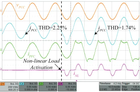
crossing distortion. After the non-linear load begins, the PCC current lowers the THD (= 1.74%) due to the increase in the fundamental component.
Fig. 24 shows the transition for a step change in the
refer-vPCC
iPCC THD=2.19% iPCC THD=1.62%
iPFC PFC Load Step
iNL
Fig. 24. Experimental results: overall system behaviour for a PFC+HMF load step. The increase in the PFC load increases the fundamental component of the PCC current leading to a lower THD.
v PCC
i
PCC DPF≈1
i PFC
DPF≠1 i
[image:12.612.59.329.253.415.2]NL
Fig. 25. Experimental results: PFC+HMF behavior when the non-linear load has displacement factor different from unity.
ence currentivDCP F C of the PFC from 50% to 100% the rated current. Initially, the PCC current THD isT HDP CC = 2.19% and, after the PFC load step, it isT HDP CC = 1.62%. Fig. 25 shows the HMF of the PFC in the face of a non-linear load with displacement factor different from unity. The PFC+HMF puts the PCC current in phase with the PCC voltage with
T HDP CC = 1.87%.
The low-frequency spectra of the grid current at the PCC
iP CC are shown in Figs. 26 and 27, for half and full power consumption in the PFC respectively. It can be seen that the HMF works in both cases with better THD for higher load as expected.
Finally, Fig. 28 shows the behavior of the PFC+HMF when the DC-link voltage control loop is present. The DC-voltage transient lasts longer than in the previous simulation because the PI controller of the DC-voltage in the prototype has a lower bandwidth, however this does not affect the performance of the HMF. Without the HMF, there is a PCC current with
[image:12.612.77.553.260.427.2] [image:12.612.51.297.464.626.2]Fig. 26. Experimental results: Steady state response of currentsiP F C,iN L
[image:13.612.50.299.260.405.2]andiP CC. Low-frequency spectrum of the currentiP CC for low power.
Fig. 27. Experimental results: Steady state response of currentsiP F C,iN L
andiP CC. Low-frequency spectrum of the currentiP CC for full power.
Harmonic Migitation Activation vdc
vPCC
iNL
iPFC
iPCC THD=3.91% iPCC
THD=24.7%
Fig. 28. Experimental results: PFC+HMF when the DC-voltage control loop is present.
VIII. CONCLUSION
The paper proposes the control design of a PFC with harmonic mitigation function for being employed in small hybrid AC/DC buildings. The proposed controller is comprised of a current reference generator, a PR controller, and a PLL. The current reference generator for the harmonic mitigation function was explained along with the limitations of the
pro-cedure. It was shown that, because of its unidirectionality, the single-phase PFC rectifier needs to consume active power for performing the HMF. The PFC rectifier used a PR controller by inferring the output current without needing additional sensors in the rectifier, which allowed proper tracking of the fundamental component. An efficient implementation for the SOGI-PLL that enables fast execution is presented. The paper provided full guidelines on obtaining all the necessary param-eters for a computationally efficient control of the PFC+HMF. The experiments presented showed that the PFC+HMF is able to reduce the THD of the PCC current from T HDP CC = 24.7%due to a high crest factor load toT HDP CC = 3.91%, complying with the norms. The proposed scheme utilizes the installed hardware and only requires software modification and the addition of a single external sensor to measure the non-linear load. Therefore, the proposed PFC+HMF presents an economically attractive option for reducing the harmonic production of small hybrid AC/DC buildings.
REFERENCES
[1] B. Wunder, L. Ott, M. Szpek, U. Boeke, and R. Weis, “Energy efficient dc-grids for commercial buildings,” in2014 IEEE 36th Int. Telecommun. Energy Conf. (INTELEC), Sept 2014, pp. 1–8.
[2] E. Waffenschmidt and U. Boeke, “Low voltage dc grids,” inProc. of 2013 35th Int. Telecommun. Energy Conf. ’Smart Power and Efficiency’ (INTELEC),, Oct 2013, pp. 1–6.
[3] Y. W. Li and J. He, “Distribution system harmonic compensation methods: An overview of dg-interfacing inverters,”Industrial Electronics Magazine, IEEE, vol. 8, no. 4, pp. 18–31, Dec 2014.
[4] S. Munir and Y. W. Li, “Residential distribution system harmonic compensation using pv interfacing inverter,” IEEE Trans. Smart Grid, vol. 4, no. 2, pp. 816–827, June 2013.
[5] K. Wada, H. Fujita, and H. Akagi, “Considerations of a shunt active filter based on voltage detection for installation on a long distribution feeder,” in Industry Applications Conference, 2001. Thirty-Sixth IAS Annual Meeting. Conference Record of the 2001 IEEE, vol. 1, Sept 2001, pp. 157–163 vol.1.
[6] T.-L. Lee, P.-T. Cheng, H. Akagi, and H. Fujita, “A dynamic tuning method for distributed active filter systems,”Industry Applications, IEEE Transactions on, vol. 44, no. 2, pp. 612–623, March 2008.
[7] P.-T. Cheng and T.-L. Lee, “Distributed active filter systems (dafss): A new approach to power system harmonics,”IEEE Trans. Ind. Appl., vol. 42, no. 5, pp. 1301–1309, Sept 2006.
[8] D. Ward, “The impact of distribution system design on harmonic limits,” inPower Engineering Society 1999 Winter Meeting, IEEE, vol. 2, Jan 1999, pp. 1110–1114 vol.2.
[9] T. Gonen, Electric Power Distribution System Engineering, Second Edition, ser. Electrical Engineering. Taylor & Francis, 2007. [10] L. Huber, Y. Jang, and M. Jovanovic, “Performance evaluation of
bridgeless pfc boost rectifiers,”IEEE Trans. Power Electron., vol. 23, no. 3, pp. 1381–1390, May 2008.
[11] F. Musavi, M. Edington, W. Eberle, and W. Dunford, “Evaluation and efficiency comparison of front end ac-dc plug-in hybrid charger topologies,”IEEE Trans. Smart Grid,, vol. 3, no. 1, pp. 413–421, March 2012.
[12] Y.-S. Kim, W.-Y. Sung, and B.-K. Lee, “Comparative performance analysis of high density and efficiency pfc topologies,” IEEE Trans. Power Electro., vol. 29, no. 6, pp. 2666–2679, June 2014.
[13] A. Leon, H. Valderrama-Blavi, J. Bosque-Moncusi, and L. Martinez-Salamero, “A high voltage sic-based boost pfc for led applications,”
IEEE Trans. Power Electron., vol. PP, no. 99, pp. 1–1, 2015. [14] S. Kim and P. Enjeti, “A modular single-phase power-factor-correction
scheme with a harmonic filtering function,”IEEE Trans. Ind. Electron., vol. 50, no. 2, pp. 328–335, Apr 2003.
[15] A. Hasim and M. Saidon, “Development of a single-phase shunt active power filter using boost rectifier technique,” in 4th Student Conf. on Research and Development, SCOReD 2006., June 2006, pp. 262–265. [16] A. Hasim and M. Hamzah, “Single-phase shunt active power filter using
[image:13.612.50.298.447.609.2][17] T. I. Inc.,Digitally Controlled Bridgeless Power Factor Correction (BL PFC) Converter Using C2000 Piccolo-A Microcontroller, ser. Applicat. Report tidu312. Texas Instruments Inc., May 2014.
[18] R. Teodorescu, M. Liserre, and P. Rodriguez, Grid Converters for Photovoltaic and Wind Power Systems, ser. Wiley - IEEE. Wiley, 2011. [19] G. Escobar, M. Hernandez-Gomez, P. Martinez, and M. Martinez-Montejano, “A repetitive-based controller for a power factor precom-pensator,”IEEE Trans. Circuits and Systems I: Regular Papers, vol. 54, no. 9, pp. 1968–1976, Sept 2007.
[20] G. Escobar, A. Stankovic, and D. Perreault, “Regulation and compen-sation of source harmonics for the boost converter-based power factor precompensator,” inIEEE 32nd Annu. Power Electron. Specialists Conf., 2001. PESC. 2001, vol. 2, 2001, pp. 539–544 vol.2.
[21] R. Teodorescu, F. Blaabjerg, U. Borup, and M. Liserre, “A new control structure for grid-connected lcl pv inverters with zero steady-state error and selective harmonic compensation,” inNineteenth Annu. IEEE Appl. Power Electron. Conf. and Expo., APEC ’2004., vol. 1, 2004, pp. 580– 586 Vol.1.
[22] P. Mattavelli, “Synchronous-frame harmonic control for high-performance ac power supplies,”IEEE Trans. Ind. Applicat., vol. 37, no. 3, pp. 864–872, May 2001.
[23] S. Fukuda and T. Yoda, “A novel current-tracking method for active filters based on a sinusoidal internal model [for pwm invertors],”IEEE Trans. Ind. Applicat., vol. 37, no. 3, pp. 888–895, May 2001. [24] A. Yepes, F. Freijedo, O. Lopez, and J. Doval-Gandoy,
“High-performance digital resonant controllers implemented with two integra-tors,”IEEE Trans. Power Electron., vol. 26, no. 2, pp. 563–576, Feb 2011.
[25] A. Yepes, F. Freijedo, J. Doval-Gandoy, O. Lopez, J. Malvar, and P. Fernandez-Comesana, “Effects of discretization methods on the per-formance of resonant controllers,”IEEE Trans. Power Electron., vol. 25, no. 7, pp. 1692–1712, July 2010.
[26] D. Zmood and D. Holmes, “Stationary frame current regulation of pwm inverters with zero steady-state error,” IEEE Trans. Power Electron., vol. 18, no. 3, pp. 814–822, May 2003.
[27] M. Kazmierkowski, R. Krishnan, and F. Blaabjerg, Control in Power Electronics: Selected Problems, ser. Academic Press series in engineer-ing. Academic Press, 2002.
[28] P. Rodriguez, A. Luna, I. Candela, R. Teodorescu, and F. Blaabjerg, “Grid synchronization of power converters using multiple second order generalized integrators,” in34th Annu. Conf. of IEEE Ind. Electron., 2008. IECON 2008., Nov 2008, pp. 755–760.
[29] M. Ciobotaru, R. Teodorescu, and F. Blaabjerg, “A new single-phase pll structure based on second order generalized integrator,” in37th IEEE Power Electron. Specialists Conf., 2006. PESC ’06., June 2006, pp. 1–6. [30] S. Kim and P. Enjeti, “Control strategies for active power filter in three-phase four-wire systems,” inFifteenth Annu. IEEE App. Power Electron. Conf. and Expo., APEC 2000., vol. 1, 2000, pp. 420–426 vol.1. [31] H. Akagi, “New trends in active filters for power conditioning,”IEEE
Trans. Ind. Appl., vol. 32, no. 6, pp. 1312–1322, Nov 1996.
[32] L. Asiminoaei, F. Blaabjerg, and S. Hansen, “Detection is key - harmonic detection methods for active power filter applications,”IEEE Ind. Appl. Mag., vol. 13, no. 4, pp. 22–33, July 2007.
[33] F. Z. Peng, “Application issues of active power filters,”IEEE Ind. Appl. Mag., vol. 4, no. 5, pp. 21–30, Sep 1998.
[34] L. Malesani, P. Mattavelli, and S. Buso, “On the applications of active filters to generic loads,” inProc. 8th Int. Conf. on Harmonics and Quality of Power, vol. 1, Oct 1998, pp. 310–319 vol.1.
[35] P. Mattavelli, “A closed-loop selective harmonic compensation for active filters,”IEEE Trans. Ind. Appl., vol. 37, no. 1, pp. 81–89, Jan 2001. [36] H. Yi, F. Zhuo, Y. Zhang, Y. Li, W. Zhan, W. Chen, and J. Liu, “A
source-current-detected shunt active power filter control scheme based on vector resonant controller,”IEEE Trans. Ind. App., vol. 50, no. 3, pp. 1953–1965, May 2014.
[37] P. C. Todd,UC3854 Controlled Power Factor Correction Circuit Design, ser. Unitrode Applicat. Note slua144. Texas Instruments Inc., Dec 1999. [38] H. Abu-Rub, M. Malinowski, and K. Al-Haddad,Power Electronics for Renewable Energy Systems, Transportation and Industrial Applications. Wiley, 2014.
[39] G. F. Franklin, M. L. Workman, and D. Powell, Digital Control of Dynamic Systems, 3rd ed. Boston, MA, USA: Addison-Wesley Longman Publishing Co., Inc., 1997.
[40] X. Wang, F. Blaabjerg, and P. C. Loh, “Virtual rc damping of lcl-filtered voltage source converters with extended selective harmonic compensation,”IEEE Trans. Power Electron., vol. 30, no. 9, pp. 4726– 4737, Sept 2015.
[41] V. Blasko and V. Kaura, “A new mathematical model and control of a three-phase ac-dc voltage source converter,”IEEE Trans. Power Electron., vol. 12, no. 1, pp. 116–123, Jan 1997.
[42] R. Raut and N. Swamy,Modern Analog Filter Analysis and Design: A Practical Approach. Wiley, 2011.
[43] J. Matas, M. Castilla, J. Miret, L. Garcia de Vicuna, and R. Guzman, “An adaptive prefiltering method to improve the speed/accuracy tradeoff of voltage sequence detection methods under adverse grid conditions,”
IEEE Trans. Ind. Electron., vol. 61, no. 5, pp. 2139–2151, May 2014. [44] J. E. Volder, “The cordic trigonometric computing technique,” IRE
Trans. Electron. Comput., vol. EC-8, no. 3, pp. 330–334, Sept 1959. [45] J. Vankka, Digital Synthesizers and Transmitters for Software Radio.
Springer, 2005.
[46] B. Sun,Designing a UCD3138 Controlled Bridgeless PFC, ser. Appli-cation Report slua713. Texas Instruments Inc., April 2014.
[47] R. Dorf and R. Bishop, Modern Control Systems. Pearson Prentice Hall, 2008.
Rafael Pe ˜na AlzolaRafael Pe˜na-Alzola received the combined licentiate and M.Sc. degree in industrial engineering from the University of the Basque Coun-try, Bilbao, Spain, in 2001, and the Ph.D. degree from the National University for Distance Learning, UNED, Madrid, Spain, in 2011. He has worked as an electrical and control engineer for several compa-nies in Spain. From September 2012 to July 2013, he has been Guest Postdoc in the Department of Energy Technology at Aalborg University, Aalborg, Denmark.
Since August 2014 he is Postdoc Research Fellow at the Department of Electrical and Computer Engineering at The University of British Columbia (UBC) in Vancouver, Canada. His research interests are energy storage, LCL-filters, solid-state transformers and innovative control techniques for power converters.
Marco Andr´es Bianchi Marco Andr´es Bianchi (S’14) was born in Neuquen, Argentina. He received the Ing. degree in electronics engineering from the National University of Comahue, Neuquen, Ar-gentina, in 2013. He is currently working toward the M.A.Sc. degree at University of British Columbia, Vancouver, BC, Canada.
His research interests include the study of linear and non-linear control techniques for power elec-tronic converters in DC microgrids.
Martin Ordonez Martin Ordonez (S02M09) was born in Neuquen, Argentina. He received the Ing. degree in electronics engineering from the National Technological University, Cordoba, Argentina, in 2003, and the M.Eng. and Ph.D. degrees in elec-trical engineering from the Memorial University of Newfoundland (MUN), St. Johns, NL, Canada, in 2006 and 2009, respectively.
He is currently the Canada Research Chair in Power Converters for Renewable Energy Systems and Assistant Professor with the Department of Electrical and Computer Engineering, University of British Columbia, Van-couver, BC, Canada. He was an adjunct Professor with Simon Fraser University, Burnaby, BC, Canada, and MUN. His industrial experience in power conversion includes research and development at Xantrex Technology Inc./Elgar Electronics Corp. (now AMETEK Programmable Power in San Diego, California), Deep-Ing Electronica de Potencia (Rosario, Argentina), and TRV Dispositivos (Cordoba, Argentina). With the support of industrial funds and the Natural Sciences and Engineering Research Council, he has contributed to more than 90 publications and R&D reports.