Using GIS databases to simulate night light imagery

Rochester Institute of Technology

RIT Scholar Works

Theses Thesis/Dissertation Collections

8-14-2012

Using GIS databases to simulate night light imagery

Joshua Zollweg

Follow this and additional works at:http://scholarworks.rit.edu/theses

This Thesis is brought to you for free and open access by the Thesis/Dissertation Collections at RIT Scholar Works. It has been accepted for inclusion in Theses by an authorized administrator of RIT Scholar Works. For more information, please [email protected].

Recommended Citation

Using GIS Databases to Simulate Night Light Imagery

by

Joshua D. Zollweg

B.S. Rochester Institute of Technology, 2010

A thesis submitted in partial fulfillment of the

requirements for the degree of Master of Science

in the Chester F. Carlson Center for Imaging Science

Rochester Institute of Technology

August 14, 2012

Signature of the Author

Accepted by

CHESTER F. CARLSON CENTER FOR IMAGING SCIENCE

ROCHESTER INSTITUTE OF TECHNOLOGY

ROCHESTER, NEW YORK

CERTIFICATE OF APPROVAL

M.S. DEGREE THESIS

The M.S. Degree Thesis of Joshua D. Zollweg has been examined and approved by the

thesis committee as satisfactory for the thesis required for the

M.S. degree in Imaging Science

Dr. David W. Messinger, Thesis Advisor

Dr. Michael G. Gartley

Dr. Emmett J. Ientilucci

Date

THESIS RELEASE PERMISSION

ROCHESTER INSTITUTE OF TECHNOLOGY

CHESTER F. CARLSON CENTER FOR IMAGING SCIENCE

Title of Thesis:

Using GIS Databases to Simulate Night Light Imagery

I, Joshua D. Zollweg, hereby grant permission to Wallace Memorial Library of

R.I.T. to reproduce my thesis in whole or in part. Any reproduction will not be for

commercial use or profit.

Signature

Date

Using GIS Databases to Simulate Night Light Imagery

by

Joshua D. Zollweg

Submitted to the

Chester F. Carlson Center for Imaging Science in partial fulfillment of the requirements

for the Master of Science Degree at the Rochester Institute of Technology

Abstract

The Digital Imaging and Remote Sensing Image Generation (DIRSIG) model and other image simulators provide the ability to utilize detailed, artificial scenes to generate spectrally and spatially realistic simulated imagery. Simulated imagery is useful in a myriad of ways, such as sensor modeling, algorithm performance as-sessment, and others. Actually making synthetic scenes, however, is often a time consuming process, requiring the manual placement of the many objects required to define the scene. This is particularly true for scenes of large spatial extent. Proposed is a technique to generate large-area night scenes for DIRSIG. This is accomplished by using freely available Geographic Information System (GIS) data to inform the placement of street light sources. Results to this point have demonstrated that this technique is a feasible way to model the radiance for large urban areas. This de-termination was made through comparison to real night time data collected by the Visible Infrared Imaging Radiometer Suite (VIIRS). The methodology is presented as a modular framework, so that future researchers can recreate the work done do this point, with the ability to easily substitute components of the workflow, such as using an alternate source of GIS data or a different simulation environment.

Acknowledgements

I would first like to extend my thanks to my helpful and patient advisor Dr. Mike Gartley. Mike was always available to answer any questions I had and also helped me to get on my feet with DIRSIG. Dr. David Messinger also deserves thanks, not only for graciously serving as my official advisor, but also for being an excellent source of useful insights and suggestions. Finally, Dr. Emmett Ientilucci deserves appreciation for his own simulation work in DIRSIG, which proved to be of great value to me. He also greatly eased the pain of writing this thesis by providing a front matter generation template for LA_TEX.

This is dedicated to my parents, Matt and Cathy, and to my sister Hannah. I also dedicate this to my Aunt Carrie, who’s support and example have allowed me to come as far as I have.

Contents

1 Introduction 13

2 Background 16

2.1 The Urbanization-Radiance Relation . . . 16

2.1.1 Using DMSP-OLS to Define City Footprints . . . 18

2.1.2 Regional Variation in Urbanization-Radiance Relation . . . 21

2.2 The Garstang Model . . . 24

2.3 Manual Scene Generation . . . 26

2.4 Automatic Scene Generation . . . 26

3 Methodology 29 3.1 General Framework . . . 29

3.1.1 Parsing the Data Source . . . 30

3.1.2 Preprocessing the Feature List . . . 31

3.1.3 Preparing the Simulation . . . 33

3.2 Current Implementation . . . 35

3.2.1 Downloading OSM Data . . . 35

3.2.2 Parsing OSM Data . . . 36

3.2.3 Creating DIRSIG Objects . . . 37

CONTENTS 8

3.2.4 Simulation in DIRSIG . . . 39

3.2.5 Registering Simulation to VIIRS . . . 41

4 Results 42

4.1 Other Node Types . . . 42

4.2 Residential Street Nodes . . . 45

4.3 Simulation Postprocessing . . . 51

5 Conclusions 58

6 Future Work 59

6.1 Refining Source Placement . . . 59

6.2 Refining Radiance Approximation . . . 60

List of Figures

2.1 VNIR dynamic range comparison of popular satellite systems. . . 17

2.2 Development and night lights have complementary uses. . . 17

2.3 Composite DMSP-OLS Imagery of VNIR Emissions over the US. . . 18

2.4 Normalized bandpass for DMSP-OLS. . . 19

2.5 Relationship between DMSP-OLS gain and observable radiance in the visible band. . . 20

2.6 Urban Perimeter vs Threshold Percent. . . 21

2.7 ULI vs NLI with linear fit. . . 23

2.8 The Garstang Model. . . 25

2.9 Scene Generation Considerations. . . 28

3.1 Night light generation framework, with data products in the top row and actions required by the user in the lower row. . . 30

3.2 Empirical line for a given band derived from two points of known reflectance. . . 33

3.3 Facetized (a) and shaded-surface (b) views of a DEM. . . 34

3.4 Basic structure of OSM data. . . 37

3.5 Pan sensor response and sodium-vapor lamp output. . . 40

4.1 Buildings simulation. . . 43

LIST OF FIGURES 10

4.2 Primary roads simulation of Indianapolis. . . 44

4.3 Secondary roads simulation of Indianapolis. . . 44

4.4 Landsat image of Indianapolis metropolitan area. . . 46

4.5 Residential street DIRSIG simulation. . . 46

4.6 VIIRS image of Indianapolis at night. . . 47

4.7 DIRSIG simulation of Indianapolis at night. . . 47

4.8 VIIRS image of Albuquerque at night. . . 48

4.9 DIRSIG simulation of Albuquerque at night. . . 48

4.10 Indianapolis scatter plot. . . 49

4.11 Albuquerque scatter plot. . . 49

4.12 Albuquerque linear regression. . . 50

4.13 Albuquerque quadratic regression. . . 50

4.14 Indianapolis linear regression. . . 51

4.15 Indianapolis quadratic regression. . . 51

4.16 VIIRS image of Indianapolis at night. . . 52

4.17 Indianapolis simulation after 25 smoothing operations and thresholding. 52 4.18 Indianapolis simulation after 50 smoothing operations and thresholding. 52 4.19 Indianapolis smoothed linear regression. . . 53

4.20 Indianapolis smoothed X2 linear regression. . . 53

4.21 Indianapolis smoothed and clipped linear regression. . . 53

4.22 Indianapolis Smoothed and clipped X2 linear regression. . . 53

4.23 Indianapolis smoothed quadratic regression. . . 54

4.24 Indianapolis smoothed X2 quadratic regression. . . 54

4.25 Indianapolis smoothed and clipped quadratic regression. . . 54

LIST OF FIGURES 11

4.27 VIIRS image of Indianapolis at night. . . 57

List of Tables

4.1 Albuquerque and Indianapolis regression results. . . 51

4.2 Indianapolis regression results. . . 55

Chapter 1

Introduction

Synthetic image generation (SIG) systems are of vast potential use to many who work in the remote sensing field. For instance, SIG environments allow system designers to evaluate a platform’s performance in an ideal scenario. The situation is ideal because perfect ground truth is available in a SIG, since the user actually creates and defines the scenes. In this way, SIG programs free designers from the need to always build expensive prototype systems and allocate resources for image acquisition campaigns, which may also be costly and have no guarantee of providing suitable data. These same advantages also give researchers developing algorithms ideal cases for evaluation and standardized test cases for comparing techniques. [1]

Despite all the benefits SIG provides, a significant amount of work may still be required to generate a simulated image. Often, much of this work is involved in creating the artificial scene description from which the eventual image will be rendered, after being subject to the impingement of simulated photons from a ray-tracing model. [1, 2] Indeed, it is often a time consuming task to build scenes, as objects and radiance sources integral to each scene must be placed and attributed manually. In fact, past techniques have involved using real image data as a visual template for creating a scene. [3] Although this technique can create realistic scenes on a fine scale, as the amount of detail and the spatial extent of a given scene increase, the number of objects to place grows ever larger. This subjects SIG users to constraints on the nature of scenes which may be simulated in a practical manner.

This thesis proposes a technique which is ultimately intended to free SIG users from the typically arduous task of scene construction, specifically for night scenes. To accomplish this, geographic information system (GIS) data were used to inform

CHAPTER 1. INTRODUCTION 14

the placement of light-source objects in select scenes. Since light sources are placed automatically, the user needs only to provide a digital elevation model (DEM) and a terrain reflectance map for the simulation. DEM’s and reflectance maps are easily obtained from openly available sources such as Shuttle Radar Topography Mission (SRTM) and the Landsat program. These data, in conjunction with GIS data from the Open Street Map (OSM) Project, provide all that is needed to automatically generate a night scene. What is needed is one or multiple features, such as high-ways, buildings, parking lots, or another that corresponds in extent to the spatial distribution of real night lights. Like SRTM and Landsat, anyone can obtain OSM data, since the project is open source. A useful site for OSM data acquisition is

http://open.mapquestapi.com/xapi/, from which downloads are made through a graphical user interface or through file transfer protocol. Downloaded data is for-matted in an XML-type style. These XML data sheets consist of a large number of spatial positions, called nodes, specified by latitude and longitude. Each of these nodes is attributed with one or more tags. Tags define what feature or features a node belongs to. For instance, a node may be tagged as a street, again as a resi-dential street, and possibly again as an intersection. So, there is a hierarchical set of features which can be defined by tags. Additionally, the nodes and correspond-ing feature tags defined in the OSM database are defined by its users. Since the proposed scene generation process requires minimal human intervention, scenes of vast spatial extent may be modeled. For example, several complete metropolitan areas were modeled for this effort. Though improvement is still required, to date the concept of using GIS data for automatic scene generation has been shown to have merit through this work.

CHAPTER 1. INTRODUCTION 15

apply this work in the future.

Chapter 2

Background

There is not an abundance of existing literature describing automatic scene gen-eration, particularly for night scenes. As a result, the framework developed here for automatic scene generation is largely original work. Many researchers, however, have worked on simulating night scenes or approximating city radiance using other methods. Two of these methods are the Garstang model and manual scene cre-ation. It is important to understand these approaches, as the automatic technique proposed strikes a balance between the two in terms of fidelity and ease of use.

2.1

The Urbanization-Radiance Relation

Automatically generating night light data, in the proposed framework, draws from data that relates to urbanization. While this is relatively new work, there is a long history of research addressing the reverse problem. That is, night lights data collected from platforms, like the Defence Meteorological Satellite Program Opera-tional Line Scan system (DMSP-OLS), are used to estimate the population, energy consumption, or extent of urbanization of cities. [7] DMSP-OLS data have even been used to accurately delineate urban, suburban, and rural areas. [8] DMSP-OLS has

a swath width of about 2930[km] with a nadir instantaneous field of view (IFOV) of

3.6[km]. This IFOV is somewhat coarse for evaluating the extent of urbanization,

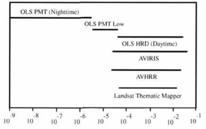
but DMSP-OLS had the advantage of more appropriate dynamic range for captur-ing night time scenes, due to its use of photomultiplier tubes. Figure 2.1 shows the dynamic range of the DMSP-OLS VNIR band compared to the VNIR bands

CHAPTER 2. BACKGROUND 17

of several other popular imaging platforms, which are intended more for capturing images during the day. [9]

Figure 2.1: VNIR dynamic range comparison of popular satellite systems.

Figure 2.2 is simple graphic showing that anthropogenic development is a driver for the night light scene simulation methodology investigated here, while actual night lights are used to estimate urban extent, population, or other human factors.

Figure 2.2: Development and night lights have complementary uses.

CHAPTER 2. BACKGROUND 18

lights data is exceedingly important to this study. If night light radiance can be used to approximate urbanization, than it should be possible to approximate night lights radiance given data relating to urbanization. The driving hypothesis of this work is exactly that, that given appropriate anthropogenic metrics, cities may be spatially and radiometrically simulated in a realistic way. The workflow described in this paper was developed to investigate what, if any, types of GIS data validated the hypothesis.

2.1.1

Using DMSP-OLS to Define City Footprints

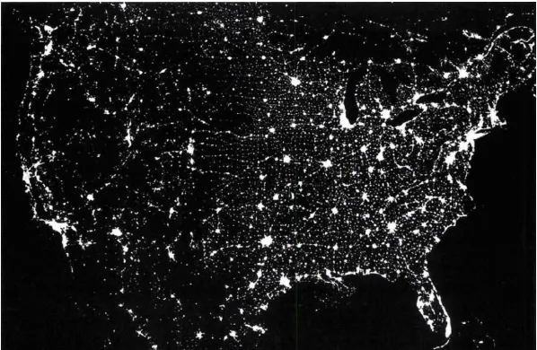
It is informative for the purposes of this project to understand how information relating to urban sprawl is interrogated from night lights imagery. Most studies in this vein utilized the DMSP-OLS satellites. This array of satellites has been in operation since the 1970’s. Although not its original mission, scientists noticed that images acquired by these satellites were able to identify lights from man-made sources, notably lights from cities, towns, and roads. [10]

Figure 2.3: Composite DMSP-OLS Imagery of VNIR Emissions over the US.

Figure 2.3 shows a composite image, which is the standard way to work with OLS data. [10] This is due to the confluence of the inherent design of DMSP-OLS, with the complications of collecting real data. The broadband panchromatic

CHAPTER 2. BACKGROUND 19

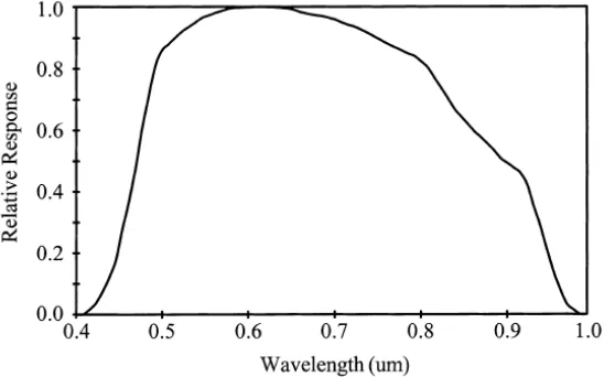
to collect images at night. Figure 2.4 shows the normalized response of the visible band for DMSP-OLS. [11]

Figure 2.4: Normalized bandpass for DMSP-OLS.

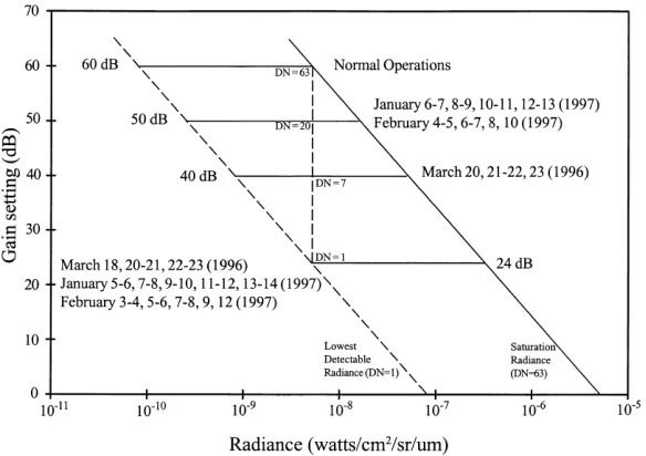
The use of a photomultiplier tube (PMT) allows these satellites to detect radiance as low as 10−10_[W/cm2_{/sr/µm]. [11] Unfortunately, the gain applied to the PMT is}

automatically adjusted and unrecorded, making the conversion from digital counts to radiance problematic. Additionally, the effective ground sampling distance (GSD) of the sensor is 2.7[km], increasing at the edges of the scan. The cross-track swath

width is 3000[km]. Large area spatial averaging and high sensitivity causes pixels

to saturate over nearly all cities. [12] Figure 2.5 plots the lowest-detectable and sat-uration radiances for DMSP-OLS under varying gain regimes. [11] When operating with zero gain, the visible ban will saturate between 10−6 _{and 10}−5_[W/cm2_/sr/µm].

Frequent saturation, of course, makes quantitative analysis of DMSP-OLS data quite difficult. Even if saturation were not an issue, the coarse radiometric reso-lution of these systems would be. DMSP sensors have only six-bits of radiometric resolution, or 64 gray levels, for the VIS sensor. [13] Technical limitations notwith-standing, using single collects would be problematic due to the presence of obscuring clouds and other phenomena.

CHAPTER 2. BACKGROUND 20

Figure 2.5: Relationship between DMSP-OLS gain and observable radiance in the visible band.

to the percentage of illumination detection, based on the number of usable collections obtained for that pixel. [14] Digital counts, therefore, typically range from 0−100. This process suppresses the influence of ephemeral light sources, such as fire, while preserving light sources of a more permanent nature. [12]

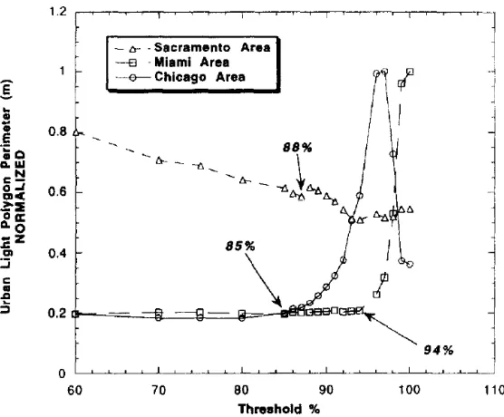
Thresholding is the default process for delineating urban areas. Imhoff et al. applied a single threshold to separate urban from nonurban areas. [12] For his work, a threshold of 0 percent included the entire image, while a threshold of 100 percent encircled only pixels illuminated in 100 percent of clear collects. A threshold of 89 percent was determined to be the baseline discriminant for US cities, based on careful analysis of Miami, Chicago, and Sacramento. This threshold was the result of averaging the ideal threshold for each of the three cities considered. The threshold for each of these cities was determined by observing where the enclosed perimeter of each began to increase rapidly as the threshold percent was increased. The large rise is attributed to the cities beginning to segment into many small polygons as opposed to just one. Imhoff’s thresholding plot is shown in Figure 2.6. [12]

CHAPTER 2. BACKGROUND 21

Figure 2.6: Urban Perimeter vs Threshold Percent.

night lights and urbanization. Although work of this variety estimates built-up area from illumination, it should be possible to do the reverse, which is the exact goal of the proposed scene generation approach in this thesis. There have been many other researchers who have done work similar to Imhoff’s for different cities all over the world. Importantly, the direct night lights-urbanization relationship holds in each case, although, there is significant variation for cities of disparate economic means or geography.

2.1.2

Regional Variation in Urbanization-Radiance Relation

CHAPTER 2. BACKGROUND 22

Surprisingly, in the same paper, Roychowdhury found that a threshold of about 20 percent was ideal for the city of Maharashtra, also in India. [8] An earlier study by Imhoff, who also used DMSP-OLS data, showed that the optimum threshold for isolating the urban core of cities in the United States was, on average, 89 percent. [12] Amaral et al. found that 30 percent was idea for Brazil. [16]

Even within one nation, differences in the structure and economy of individual cities alter the exact nature of the urbanization-night lights relationship. Yang et al. demonstrated this fact when examining urbanization in China. [15] As with the other studies, DMSP-OLS was used to identify urban areas. Yang cleverly used these data over China to create a night lights index (NLI). The NLI is a linear

combination of two components, the first is the mean light intensity index “I” and

the second is the light area index “S.” The mathematical descriptions of I and S,

respectively, are given by

I =

63

P

i=1

(DNi×ni)

N ×63 (2.1)

S = AreaN

Area . (2.2)

In Equation 2.1, DNi is the digital count equal to i, ni number of pixels of DN

equal to i, and N is the number of pixels with nonzero DN’s (illuminated pixels).

In Equation 2.2 AreaN is the area of illuminated pixels and Area is the area of all

pixels.

Components I and S are then combined linearly to create the NLI. Final NLI

shows the combination of I and S and is given by

N LI =w1I+w2S. (2.3)

Variables wI and wS are the weights for I and S. The weights assigned to each

component are adjustable, with the total weight from both components summing to one.

CHAPTER 2. BACKGROUND 23

U LI =

5

X

i=1

(wi ×Ai). (2.4)

Each weight, wi for i = 1to5, was set to equal 0.2. This assumes an equal

contribution from each statistic.

Finally, regression analysis was performed comparing ULI to each of the possible

NLI’s. The NLI constructed with w1 = 0.9 and w2 = 0.1 proved to offer the best

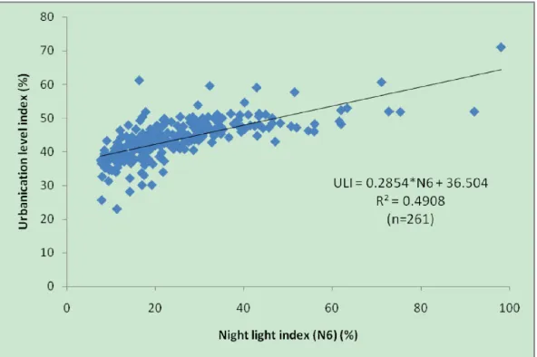
fit for China as a whole. Figure 2.7 shows the linear fit achieved by Yang. In other words, light intensity index, I, is favored heavily over light area index, S. [15] Adjustments to the slope and intercept of the linear fit between ULI and NLI improve the fit for different regions of China, however, overall there is still a strong linear relationship between the level of urbanization and level of radiance upwelled into the sky from anthropogenic sources. Adapting to specific regions, in most cases, improved the nationwide R2 _{fit of around 0.49 to a 0.60, or more. This correlation}

is key for the proposed method of automatically generating night lights. Regional variation indicates that measures may need to be taken to assure accurate simulation for a wide variety of cities.

CHAPTER 2. BACKGROUND 24

2.2

The Garstang Model

Urban glow is not solely a concern of those in the remote sensing field. Astronomers also have cause to be concerned with radiance emanating from cities, though for rather different reasons. Whereas city light data is celebrated by remote sensors for its abilities to analyse human development, stargazers see such radiance as a serious hindrance to their work. “Light pollution” is the preferred term in astronomical circles and refers to the overall brightening of the sky due to artificial lighting. Light pollution is a problem because light from man-made sources does not simply travel up and away from Earth. In fact, this light scatters through the atmosphere, brightening it, making observation of stars and other celestial phenomena more difficult. [4]

Garstang developed a model which allows for prediction of brightness in the night sky at a specified zenith angle and distance from a city. [6] The Garstang model is significant to the purposes of this paper because it represents an early attempt to predict city radiance. Furthermore, the city radiance for the model is approximated by using a given city’s population. Although the model proposed here does not use population data, it draws from GIS data which also reflect anthropogenic factors, namely level of development.

In the Garstang model, the city itself is represented as a single large circular area source. The radius of this city disk is approximated from atlases or maps, while its brightness is determined in a parametric fashion, based on the correlation between the population of a city and the brightness being upwelled from that city. Approximating a city as a single source is fine for astronomers, who do not look directly at cities. Astronomers look upwards into the sky and therefore are only concerned with the effects of light scattered from cities into the atmosphere. For remote sensing applications, it will generally be desirable to have cities be resolvable. It was Walker who originally researched and established this relationship. Walker developed the exponential relationship between population and distance from the city center asP ∝D2.5_{, whereP is population andDis distance. [5] The relationship}

between population and distance is defined as P ∝D2.5_{, where cities of population}

P produce sky brightening of 0.2 magnitude at 45◦, looking towards the city. Much

like Welch’s observations of DMSP night lights, Walker found that population and night lights were correlated. [7] Similarly, Walker was also able to establish the relationship between intensity I and distanceD as I ∝D−2.5.

CHAPTER 2. BACKGROUND 25

the prediction of intensity at arbitrary zenith angles and distances. The model is represented schematically as shown in Figure 2.8. [6]

Figure 2.8: The Garstang Model.

The governing equation of the Garstang model is given as

Iup=

LP

2π

n

2G(1−F) cos Φ + 0.554FΦ4o. (2.5)

Here, P is the population, R is the city radius, L is the lumens produced per

person, F is the fraction of light radiated upwards into the sky, Φ is the zenith

angle to the observation altitude, and Gis the of light radiated towards the ground,

(1−F), that is reflected into the sky in a Lambertian fashion. So, this model only

addresses first bounce radiance coming from the ground. Also noteworthy is the Φ4

term, which is selected because of its similarities to modelling the actual radiance distribution of most street lights, which have nearly zero radiance directly above the light, but have greatly increasing radiance with increasing zenith. [6]

CHAPTER 2. BACKGROUND 26

2.3

Manual Scene Generation

Manually creating a scene allows for an exceedingly high level of detail to be mod-eled. If taken to the extreme, a scene can more or less be constructed as an exact replica of a real location. The synthetic creation could have accurately created ge-ometries for buildings, trees, street lights, and whatever else is put into the scene. Similarly, all scene materials would be appropriately attributed with the correct ma-terial properties, such as reflectance, and specific source terms, like a sodium vapor street light, an incandescent floodlight on a home, or other types of illumination.

Having such control over the simulated world is very useful and allows for many minute adjustments to be made for nuanced and well controlled experiments. The price of this control is the time it takes to build this sort of scene. If it is a real location that is being recreated, highly accurate ground truth must be collected. Next, all the required objects must be acquired or created and then carefully placed to correspond with ground truth. The whole process is very labor intensive and time consuming.

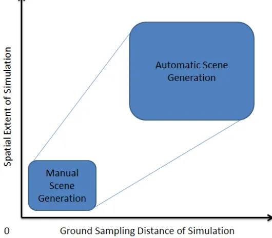
It is easy to imagine that the amount of set-up work required will increase quickly as the size of the scene being built grows larger. As a result, manually building a highly realistic scene generally relegates the creator to a relatively small extent. There are a huge variety of applications where this is perfectly acceptable, because high accuracy is required. It is unlikely that any automatic scene generation scheme will ever be able to replace the need for manually constructed scenes. That said, however, there are certain tasks where using lower fidelity, but quicker, automatic scene generation for larger extents may be acceptable.

2.4

Automatic Scene Generation

CHAPTER 2. BACKGROUND 27

circular extended source. Naturally, for a downward-looking imaging application a single source is not acceptable, given that the image’s resolution is smaller than the city in question. So, the question of how to spatially place a large number of sources in an accurate fashion remains.

Automatic scene generation was conceived as a way to avoid having to make arbitrary heuristic decisions and to save a user time. The basic concept is that there should be a source of data which is correlated with what must be modeled. In the case considered here, the conjecture was that some component of GIS data should relate somehow to man-made illumination sources. This was assumed because ear-lier studies, some of which were described here, demonstrated strong correlation between urbanization and nighttime radiance. Since GIS data includes information regarding the location of urban features, it should be a suitable driver for automat-ically creating a simulation of night lights. Since simple light sources are used and placed based on features related to lighting, and not the explicit positions of lights themselves, this approach is less realistic than manual scene generation. Again, its advantage lies in striking a balance between fidelity and creation time for large scenes.

CHAPTER 2. BACKGROUND 28

Chapter 3

Methodology

At the top level, there are only a few key steps required to generate simulated night light imagery. This allows the entire process to be summarized as a general framework. In this preliminary investigation, specific choices were made along each step of the general workflow. Of course, there exists an enormous range of different options for producing night light imagery. Hopefully, the framework presentation allows future investigators to easily implement their own novel approaches, without excessive logistical problems. Certainly, parts of the existing workflow could simply be switched out for a new technique, while still making use of the remaining work-flow. Another benefit of the established workflow is that the current source of GIS data, Open Street Map (OSM), can be substituted for another, if the need arrives.

3.1

General Framework

Once a user has selected a data source and acquired the data to be used for a simulation, there are three primary actions needed. These three actions include parsing the data, preprocessing the data, and setting up the desired simulation. If the data source used corresponds closely to the spatial distribution of night lights and light sources are attributed based on that distribution in the correct proportions, then an accurate simulation should be expected. Finding data which relates closely to the spatial distribution of real night lights and defining source objects based on that distribution is the most difficult part of this work. It is likely that many different sources of data will need to be tested. A general framework for processing

CHAPTER 3. METHODOLOGY 30

helps to make this process of experimentation more efficient. Sections 3.1.1, 3.1.2, and 3.1.3 describe these three steps in greater detail.

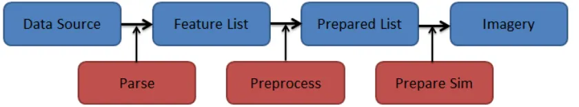
Figure 3.1 provides a visual interpretation of the workflow. Actions required by the user occupy the bottom row and are colored in red. The states of the data preceding and following each action occupy the top row and are colored in blue. Raw data, perhaps OSM, shapefile, or KML data, must first be parsed to find and identify only the parts of that data which are pertinent to the simulation. This pro-cess produces a feature list of the relevant data. The feature list may included road networks, buildings, the extent of classified regions, or any type of feature which may be appropriate for modeling night lights. The list consists of the locations of each instance of the feature type, or types, being investigated. Simulation suites like DIRSIG or the PRA Toolkit often require specifically formatted files to describe where and what type of objects will occupy the scene being simulated. The prepro-cessing step generates the prepared list by doing a coordinate transform, while also aggregating sources (if necessary, described in detail in Section 3.2.3), and assigning each aggregated or indvidual feature instance an object type. Generally, this object type will be an emission source of somekind, like a streetlight with a defined emis-sion spectrum. This prepared list should be formatted properly for use with the simulation software being used and written to a file. Finally, the simulation must be prepared. Generally this involves defining an imaging platform’s sensing abilities, its position, and potentially its flightpath.

Figure 3.1: Night light generation framework, with data products in the top row and actions required by the user in the lower row.

3.1.1

Parsing the Data Source

conver-CHAPTER 3. METHODOLOGY 31

sion. Additionally, not all of the information contained in a file will be needed for the simulation. Blindly including all points defined by a large source of data is not likely to return a realistic output. As a result of these two factors, it is generally necessary to parse the raw data into an intermediate format or feature list. A feature list should contain only nodes with the tags desired for the given simulation.

A benefit of parsing the data is searchability. GIS databases such as Open Street Map provide data in an XML-like format, which is not quickly readable. Other data formats have similar issues. Shapefiles, for instance, store instances of primitive shapes and points separately from attributes which describe those points. Searching the shapefile and referencing shapes to attributes is not efficient. So, in most cases, it is best to take the time to parse a data source once to build a quickly searchable list. The parsed list may be saved as a unique file for future use.

During the parsing process, it can also be good practice to save only the types of features, or node types (different tags), which are of interest for the current simulation experiment. This can be accomplished during the parsing process by referencing each feature instance to the tags or attributes which define it. Or, the entire file can be parsed and saved. Then, that file can be quickly searched to extract whatever the desired feature or features may be for future simulations. The primary goal of this step is to create a file which is easily and quickly searchable in a programming environment, which will eventually end up being a significant time-saving measure.

3.1.2

Preprocessing the Feature List

The feature list is essentially a more relevant and usable version of the source data. It will generally not be ingestible by the chosen simulation environment at this point. The preprocessing step addresses this shortcoming.

Specifics of the preprocessing required will depend on what format the original data was parsed into and what image simulation tool is being used. Generally, this step will consist of coordinate transformations and formatting an input file for the image simulator. It is meant to serve as a coupling between input data and the simulator.

CHAPTER 3. METHODOLOGY 32

practicality and what can actually be simulated in a reasonable timeframe. Others will be experimental in nature, in order to try and generate an accurate model of night lights.

The method by which data points are processed will have a large effect on the nature of the resulting simulation. For instance, should each relevant data point be treated as an individual source in the simulation? Should point sources or area sources be used? Maybe different types of data points should be associated with different illumination types. Perhaps a more realistic result may be achieved by looking for specific groupings of different varieties of data points and assigning source types and intensities based on that criteria. Ultimately, it is difficult to know from the onset what approaches will generate the most realistic result. Different sources of input data may be intrinsically very different from one another and require very different techniques for generating accurate simulations. In addition to adjusting the methodology based on the available input data, practical considerations must also be made during the preprocessing phase.

CHAPTER 3. METHODOLOGY 33

3.1.3

Preparing the Simulation

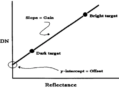
Although the terrain itself is not typically visible in night imagery, it is generally good practice to have realistic ground cover. The reason for this is that most man-made light sources do not point directly up at the sky. Street lights point downwards, so the majority of visible illumination is actually reflected off the ground before propagating upwards through the atmosphere. To account for this, it is good to use a reflectance map as an image background. If there are no available reflectance maps for a given area, it is possible to create one. A useful approach is to acquire Landsat data and use some of ENVI’s built-in processing tools, such as the empirical line method (ELM) to create a rough reflectance map. ELM works by estimating a gain and offset term from two or more targets in the radiance image and is governed by

DNb =ρ(λ)Ab+Bb. (3.1)

In the equation,b specifies a given band,DN is a pixel digital count,ρ(λ) is surface

reflectance at wavelength λ, A represents the multiplicative gain, and B represents

the additive offset. [17] Figure 3.2 illustrates graphically how the emprical line is derived from two targets of known reflectance. [17] Given the proof-of-concept nature of this work, two-point ELM was deemed suitable for creating the reflectance maps. In future work, however, the workflow may need to be modified with a more rigorous reflectance conversion.

Figure 3.2: Empirical line for a given band derived from two points of known re-flectance.

CHAPTER 3. METHODOLOGY 34

good practice to address elevation changes in terrain. Usually a facetized digital elevation model (DEM) is used for this purpose. Figure 3.3 shows the facetized and shaded-surface views of an example DEM. If the DEM for a given location is not available, it is possible to create one from data such as that available from the Shuttle Radar Topography Mission (SRTM).

(a)

(b)

Figure 3.3: Facetized (a) and shaded-surface (b) views of a DEM.

CHAPTER 3. METHODOLOGY 35

3.2

Current Implementation

This section details the specific steps taken to produce simulated night lights imagery for this project. Before any other work may progress, Open Street Map (OSM) data must be downloaded from the OSM servers for the region of interest. It is preferable to download the OSM data in many small pieces, as opposed to one large file. The

easiest way to do this is to use command line tools, such as UNIX’s wget. Section

3.2.1 describes the downloading procedure in greater detail. Once the OSM data are obtained, they must be parsed to extract only the nodes which will be used in the forthcoming simulation. MATLAB was selected for parsing, though in an optimized workflow, a more quickly executing language should be used. More detail on parsing is provided in Section 3.2.2. Section 3.2.3 explains how the coordinates of the relevant nodes are converted from latitude and longitude to a scene-relative East, North, Up (ENU) coordinate system, then spatially aggregated, assigned a light spectrum, and finally written to an object database (ODB) DIRSIG file, which is used by DIRSIG. MATLAB was again used for these steps. The last step in the workflow is actually running DIRSIG with the OSM-derived ODB. Generating the simulation in DIRSIG can be the bottleneck of the entire process, so simplifications

were made when possible. DIRSIG simulations finish more quickly when using

the simple atmosphere model, at the cost of radiometric accuracy. In a finalized methodology this would be unacceptable. At the current proof-of-concept stage, the sacrifice is tolerated. Section 3.2.4 describes the settings used for the DIRSIG simulations.

3.2.1

Downloading OSM Data

Xapi is the name of the online tool used to query the OSM database. Xapi is an extended OSM API that allows the acquisition of OSM data based on region and/or node type. Regions and node type may be easily selected from Xapi’s website,

http://open.mapquestapi.com/xapi/.

CHAPTER 3. METHODOLOGY 36

should be downloaded as many small tiles. For a city such as Indianapolis, between 100 and 400 tiles were used.

Though region tiling solves the parsing issue, manually selecting hundreds of regions on the Xapi site is inefficient. An iterative UNIX shell script proved to be an effective alternative. The script allows the user to enter the latitude and longitude of the region of interest, in addition to the number of desired tiles. At each iteration, wget was used to download all of the nodes for a particular tile. This approach obtains OSM data for a city region in a matter of minutes and presents it in a form more easily digestible for parsing in MATLAB.

3.2.2

Parsing OSM Data

MATLAB supports a built-in function named parseXML. This function parses an

XML document and returns a data structure in the Document Object Model (DOM)

format. Since OSM files are written in accordance with XML conventions,parseXML

is well suited for this purpose. Figure 3.4 describes the basic structure of OSM data. Each file consists of a long list of node points, which are distinguished by unique identification numbers. Each node’s location is specified in latitude and longitude. Tags add associated extra information with each node, which may be of interest to users. Ways are basically lists of nodes with their own sets of tag descriptors. These entries are included after the nodes in an OSM file. Ways are also typically assigned a class, so that they can be identified easily as roads, buildings, parking lots, sports arenas, or other features.

CHAPTER 3. METHODOLOGY 37

Figure 3.4: Basic structure of OSM data.

3.2.3

Creating DIRSIG Objects

Once the list of nodes to use is parsed from the input OSM files, the node loca-tions must be converted from latitude and longitude to an East, North, Up (ENU) coordinate system. DIRSIG ODB files require that the various objects in a scene be specified in ENU coordinates, which are relative to the location of the geodetic scene center point used for the simulation. WGS-84 is the geodetic system used.

CHAPTER 3. METHODOLOGY 38

X = (aC+h)×cos(lat) cos(lon)

Y = (aC+h)×cos(lat) sin(lon)

Z = (aS+h)×sin(lat).

(3.2)

In Equation 3.2 “a” is the WGS-84 equatorial earth radius and “h” is altitude

above sea level. Constants “C” and “S” are dependent on latitude, longitude, and

the reciprocal of the earth flattening parameter “f,”also defined by WGS-84. The

flattening parameter is a function of the equatorial and polar earth radii, “a” and

“p” respectively. Variables “f,” “C,” and “S” are defined as

1

f =

_a−b

a

−1

C = qcos2_{(lat) + (1−f)}2_sin2_(lat)−1 S = (1−f)2_C.

(3.3)

With all nodes converted to ECEF, the final conversion to ENU may commence. The origin of the DIRSIG scene must also be converted to ECEF, as it is required in the definition of ENU. The origin coordinates are specified as X0, Y0, and Z0 and

are used for centering the ECEF coordinates relative to the scene. A conversion

matrix “M” is used to convert a vector of ECEF coordinates for a given node to a

vector of ENU coordinates. The conversion operation is given by

E N U

=M ×

X−X0 Y −Y0 Z−Z0

(3.4)

with the conversion matrix “M” defined as

M =

−sin(lon) cos(lon) −sin(lat)

−sin(lat) cos(lon) −sin(lat) sin(lon) cos(lat) cos(lat)cos(lon) cos(lat) sin(lon) sin(lat)

.

CHAPTER 3. METHODOLOGY 39

objects. So, nodes are aggregated over spatial regions of the scene. The GSD

of these regions should be at most half the GSD of the imaging platform used in the simulation to prevent undersampling. Spatially aggregating nodes is beneficial because it allows spectral intensity to be binned as well. This means that if a region has 10 nodes, a single object with 10 times the brightness of the original sodium-vapor lamp is written to the ODB. This binning results in simulations which finish faster as compared to 10 individual sodium-vapor objects.

3.2.4

Simulation in DIRSIG

The ODB derived in the previous steps is used to place source objects within a scene. The scene is comprised of two components. Component 1 is a DEM, the same DEM which was used to determine the altitude of each node in Section 3.2.3. Component 2 is a reflectance map derived from Landsat 7 data. Together, these two components do an adequate job of modelling the relief and reflectance properties of the scene. These are important factors, because the light objects used point downward, in order to mimic an actual street light. As a result, much of the radiance seen in the simulation is actually reflected off the ground.

DIRSIG simulations were run for several different platform types. Ultimately,

a platform with roughly 1₃ of the ground sampling distance (GSD) of the imaging

platform used for validation was selected. This increased the runtimes of the simu-lations. Increased runtime was ultimately deemed acceptable because it allowed the resulting simulation to be viewed in detail sufficient for comparison to truth data from Open Street Map, as well as remotely sensed imagery such as that found in Google Earth. These comparisons helped to identify the strengths and weaknesses of simulations produced by the various node types. For instance, residential roads proved to be the best available node type in Open Street Map, however, there are certain urban features it omits. Airports are a prime example. Additionally, gener-ating simulations with reduced GSD is beneficial if postprocessing is performed on the synthetic night lights imagery. Likely, some fidelity is preserved by operating on a higher resolution image, before registering and interpolating down to the real VIIRS imagery.

CHAPTER 3. METHODOLOGY 40

results with high spatial correlation to night light distribution proved more difficult than expected, research never progressed to the point of finding ways to decide how to appropriately assign multiple sources. So, the prospect of creating true color images demonstrating spectrally diverse lighting was abandoned, along with the requisite red, green, and blue bands. The pan band used was modeled as being wide

open with a rectangular response function from 400[nm] to 1100[nm]. This range

includes the major peaks of spectral output for sodium-vapor lamps, the light source used for all simulations in this study. Figure 3.5 shows the pan band response and the normalized output of a vapor lamp. The spectrum used for the sodium-vapor lamp was taken from work done by Elvidge et al. [10]

Figure 3.5: Pan sensor response and sodium-vapor lamp output.

Rig-CHAPTER 3. METHODOLOGY 41

orous evaluation of the proposed methodology would require greater accuracy. All simulations were run at night with no moon.

3.2.5

Registering Simulation to VIIRS

Each completed night light image must be registered to real imagery for further analysis. The best data available for this purpose was that from the Visible Infrared Imaging Radiometer Suite (VIIRS). VIIRS has a Day/Night Band (DNB), centered at 0.7[µm] which uses multiple focal plane arrays simultaneously running at different gains. [13] This configuration grants the system vast dynamic range, seven orders of magnitude, which is beneficial when imaging night scenes. The signal is digitized and quantized using 14 (high gain) or 13 (medium and low gain) bits. So, high ra-diometric resolution accompanies the large dynamic range. With regard to spatial resolution, VIIRS has a nadir pixel GSD, or instantaneous field of view (IFOV) of 0.742[km]. Each VIIRS “pixel” is actually constructed of several smaller subpixels. These subpixels are aggregated appropriately across the field of view (FOV) to ap-proximately maintain the IFOV across the entire scan. Extreme dynamic range com-bined with high radiometric resolution and moderate spatial resolution, make VIIRS a well-suited system for verifying the radiometric and spatial accuracy of the simu-lations generated from OSM data. The unprocessed VIIRS DNB imagery used here

was acquired fromftp://is.sci.gsfc.nasa.gov/gsfcdata/npp/viirs/level1/.

VIIRS DNB imagery and other VIIRS imagery and data products are served through

http://www.nrlmry.navy.mil/VIIRS.html.

Simulation-to-image registration was accomplished in ENVI using the built-in

image-to-image registration tool. First, daylight simulations were generated in

Chapter 4

Results

Using the methodology described in Section 3, several simulations were generated for the cities of Albuquerque and Indianapolis. A key goal of this research is to identify which node types are the most useful to describe the spatial distribution of urban night lights. Many different node varieties were tested, notably primary, secondary, and residential street nodes, in addition to building and street light nodes. To determine which types among these are most suitable, individual simulations for each node type and city were run and compared to the reference VIIRS day-night band dataset. Residential street nodes proved to be best suited for simulating night lights with the OSM dataset, though refinement is required to suppress certain artifacts in the data. These results are examined in Section 4.2. Unfortunately, many of the node types that corresponded most directly to night lights were not usable for various reasons, as will be discussed in Section 4.1.

4.1

Other Node Types

After developing a workflow which can process nodes for input to DIRSIG, the next step was finding which types of nodes gave the best results. Naturally, the closer association a node type has to actual radiance, the better. An early hypothesis was that street lights contributed the greatest proportion of urban radiance. It was a pleasant surprise to find that there was actually a street light tag in Open Street Map. Unfortunately, almost no street lights were defined in the cities investigated. So, the next thought was to use the next closest relation, which is to just use roads

CHAPTER 4. RESULTS 43

themselves. Within the OSM data there are many different classifying tags for roads. These include primary, secondary, tertiary, pedestrian, residential, and service roads, to name a few. Interestingly, many of these road types are defined according to UK specifications, since Open Street Map is a UK-based project.

Figure 4.1: Buildings simulation.

CHAPTER 4. RESULTS 44

Figure 4.2: Primary roads simulation of Indianapolis.

Figure 4.3: Secondary roads simulation of Indianapolis.

Since buildings were not particularly useful as a simulation driver, it was time to turn to a type of data which Open Street Map should describe very well, streets. There are a plethora of road types which are uniquely tagged in Open Street Map and the ones which are meant for auto traffic are mapped quite completely. There are tags for foot paths and other non-motorized traffic, though these are less commonly entered into the database. Primary roads and motorways are of the largest vari-eties. These are generally federally managed toll roads, freeways, or major passages between towns. Secondary roads are defined as roads which may link smaller towns. Figures 4.2 and 4.3 illustrate the simulations produced by the primary and secondary road types, respectively. With these larger streets, the general result tends to be a web like network of very bright paths around and between cities, which inform very little about the distribution of lights within the city itself. These road types, are therefore not desirable for modeling city radiance. That said, high traffic streets are generally illuminated and many are visible from space, as DMSP-OLS and VIIRS imagery prove. If an exceedingly large scene including several metropolitan areas were simulated, these road types would have an important role to play.

CHAPTER 4. RESULTS 45

suburban areas. In the OSM database, residential street nodes do just that.

4.2

Residential Street Nodes

Residential streets proved to be a suitable individual node type for modeling night lights. These nodes are very densely distributed in urban and suburban areas, while less so in more rural areas. As a result, the spatial borders of more highly urbanized regions are well defined using residential street nodes. This node type worked better for Albuquerque than Indianapolis. Development outside of Albuquerque’s city lim-its is far more sparse than development outside of Indianapolis. More surrounding development results in a higher number of residential street nodes in rural areas. As a result, light sources are erroneously assigned in rural areas of the Indianapolis scene at a higher rate of occurrence than in the Albuquerque scene. Figure 4.6 and 4.7 illustrate the comparison between the VIIRS imagery and the simulated DIRSIG scene. While in large part the simulated and real scenes exhibit overlap in the location of light sources, false response in rural areas is plainly evident in the DIRSIG scene of Figure 4.7. Section 6 describes ways in which this problem may be alleviated.

Why, among all of the different node types tested, did residential nodes prove to be the most useful? Primary and secondary street nodes generally serve as links between cities and towns and are frequently illuminated. Simulations generated with these node types produced an extremely bright road network, but not much else. Although residential streets may not always be illuminated, or brightly illumi-nated such as larger roads, their density appears to be more highly correlated with development. The downtown region of a city has an exceedingly high amount of residential street nodes compared to a rural area, even with the Indianapolis scene. Since it is urban development that relates to night light radiance, residential streets provide the best link of any street type tested.

Unfortunately, not all node types are as thoroughly defined as street nodes. For instance, the street light node type was not commonly defined by contributors to the OSM database. Otherwise, it would have likely been useful data. Buildings

are also sparsely defined in the OSM database. This is also unfortunate, since

CHAPTER 4. RESULTS 46

Figure 4.4: Landsat image of Indianapolis metropolitan area.

Figure 4.5: Residential street DIRSIG

simulation.

large buildings often exhibit a high radiance output. For instance, many skyscrapers are commonly illuminated at the top with upward-facing sources. Such features are usually distinguishable from the average radiance level of the city. For instance, in Advanced Land Imager (ALI) data, only certain very bright features are detectable above the noise. Therefore, including these features in simulated scenes is very important. So, buildings nodes serve as a good supplement to residential street nodes, but are not enough on their own, since only very few are defined in OSM.

CHAPTER 4. RESULTS 47

Figure 4.6: VIIRS image of Indianapolis at night.

Figure 4.7: DIRSIG simulation of Indi-anapolis at night.

Figures 4.8 and 4.9 show the VIIRS and DIRSIG scenes for Albuquerque. No-tice that there is less evidence of out-of-place radiance response surrounding the city. This is attributed to there being less development surrounding Albuquerque as compared to Indianapolis.

CHAPTER 4. RESULTS 48

Figure 4.8: VIIRS image of Albuquerque at night.

CHAPTER 4. RESULTS 49

Figure 4.10: Indianapolis scatter plot. Figure 4.11: Albuquerque scatter plot.

Within urban areas, however, node density does not correlate as closely to the level of radiance.

There are other potential reasons for the general overestimation of radiance. It is possible that the sodium vapor spectra used in the simulation differs somewhat from the lamps actually used in street lights in some cities. Additionally, the simulations do no currently account other source types, such as mercury vapor lamps. Taking on-site measurements in one or more cities would help to answer these questions. Perhaps a new source spectrum could be defined which is a linear combination of different lighting types, based on measurements in real cities. This, in conjunction with defining a new scheme for attributing source objects, may provide the most appropriate solution for fixing the radiance overestimation. This solution is desirable because it would produce accurate simulations without the need to extra processing.

The current solution involves extra processing to derive a correction factor that appropriately reduces the radiance in each simulation. To estimate a correction factor, the simulated radiances in the DIRSIG scene are plotted against the observed radiance in the VIIRS scene. Next, a linear regression is performed to find the best fit to the data in a least-squares sense. The slope of this line should define the reciprocal of the correction factor for the scene in question. Division of the DIRSIG simulation radiances by the slope of the regression line should bring the radiances into closer agreement with the VIIRS data.

regres-CHAPTER 4. RESULTS 50

Figure 4.12: Albuquerque linear

regres-sion. Figure 4.13: Albuquerque quadratic

re-gression.

sion. The slope of the line for Albuquerque was determined to be approximately 86, which is in reasonable agreement with the generally observed overestimation

of roughly two orders of magnitude. The R2 for the fit was about 0.92. Figure

4.12 shows the plotted data and the regression line for Albuquerque. Figure 4.13

shows the same, but for a quadratic regression. The R2 _{fit for this plot improved to}

0.96. Both of these plots, and those which follow, are rank-order plots. VIIRS and DIRSIG pixels were individually sorted in order of ascending radiance to produce these plots and ascertain a correction function. Since both images have had their pixels sorted by different indices, nothing related to the spatial relationship of the pixels is determinable from these plots. The point of the correction functions is to bring the image radiances into general agreement, while not necessarily correcting on a pixel-to-pixel basis.

Figure 4.14 shows the regression plot for Indianapolis. Although the linear fit for

Indianapolis could be quantitatively considered “good,” with an R2_{of 0.89 and slope}

of 162, visual inspection appears to reveal a different phenomenon. At higher radi-ances, the simulation’s tendency to overestimate is exacerbated. This contributes to the steeper slope, but the trend of the data appears to be vaguely parabolic in nature, so a quadratic regression was performed. This regression, shown in Figure

4.15 fit the data exceedingly well both visually and quantitatively. The R2 _{for the}

quadratic fit was approximately 0.96. Table 4.1 summarizes the R2 _{values of the}

linear and quadratic regressions for both cities.

cor-CHAPTER 4. RESULTS 51

Figure 4.14: Indianapolis linear

regres-sion.

Figure 4.15: Indianapolis quadratic

re-gression.

rection factor for global application to the simulation is impossible. This unexpected result indicates that it may be necessary to develop unique correction functions for each simulation. Ideally, this will be done in an automated nature. The possibility of this will be determined by whether or not the variables contributing to the form of the correction functions can be associated with data available in OSM.

City Fit R2

Albuquerque Linear 0.92

Albuquerque Quadratic 0.96

Indianapolis Linear 0.89

Indianapolis Quadratic 0.96

Table 4.1: Albuquerque and Indianapolis regression results.

4.3

Simulation Postprocessing

CHAPTER 4. RESULTS 52

Figure 4.16: VIIRS im-age of Indianapolis at night.

Figure 4.17: Indianapo-lis simulation after 25

smoothing operations

and thresholding.

Figure 4.18: Indianapo-lis simulation after 50

smoothing operations

and thresholding.

that problem. This leads to source objects being assigned in error.

Several approaches were tested to try to remove the erroneous suburban/rural response in postprocessing for the Indianapolis simulation. Ideally this would be an unnecessary step, just like the radiance correction function. Until the workflow is improved, however, a simple postprocessing procedure to clean away erroneous response is desirable. Out of the investigated procedures, iterative smoothing fol-lowed by application of a threshold proved to offer the best results. Essentially,

the residential road simulation was smoothed successively by a 7x7 Gaussian

ker-nel with a σ of 0.8 and a total weight of 1. Convolving the image with the kernel

25 times seemed to sufficiently spread out the response of individual road ways such that they could be more easily thresholded. The threshold value used was 2.0×106[W/cm2/sr]. The smoothing and thresholding was applied to the simula-tions before radiance correction, in these cases. This kernel, number of smoothing iterations, and threshold were all determined heuristically. To further investigate the effects of smoothing, the simulation was also smoothed 50 times. This time a smaller threshold of 1.0×106_[W/cm2_{/sr] was most suitable.}

CHAPTER 4. RESULTS 53

Figure 4.19: Indianapolis smoothed linear regression.

Figure 4.20: Indianapolis smoothed X2 linear regression.

Figure 4.21: Indianapolis smoothed and clipped linear regression.

CHAPTER 4. RESULTS 54

Figure 4.23: Indianapolis smoothed

quadratic regression.

Figure 4.24: Indianapolis smoothed X2 quadratic regression.

Figure 4.25: Indianapolis smoothed and clipped quadratic regression.

CHAPTER 4. RESULTS 55

Each of the smoothed iterations each had a “clipped” regression performed. Here, a clipped regression refers to ignoring the points where the simulation was thersholded to zero. The large number of zero points was causing the slope of the regressions to be overly steep. Figures 4.21 and 4.22 show the clipped results, which should possess more representative linear fits.

Based on the scatter plots of the processed data, a quadratic fit may prove to be more appropriate than a linear one. This was the case with the unprocessed simulation, so it was attempted again here. Figures 4.23 and 4.26 show the resulting plots. As before, the quadratic functions fit better than the linear ones.

City Processing Fit Coefficients R2

Indy None Linear 162 0.89

Indy None Quadratic 7.42e8, 1.81e2 0.96

Indy Smooth Linear 102 0.75

Indy Smooth Quadratic -3.52e8, 1.43e2 0.83

Indy Smooth and Clip Linear 74 0.83

Indy Smooth and Clip Quadratic -1.40e8, 74.21 0.90

Indy Smooth X2 Linear 94 0.69

Indy Smooth X2 Quadratic -2.97e8, 1.42e2 0.85

Indy Smooth X2 and Clip Linear 47 0.78

Indy Smooth X2 and Clip Quadratic -1.65e8, 1.01e4 0.90

Table 4.2: Indianapolis regression results.

Table 4.2 includes the results of the linear and quadratic regressions performed on all of the different Indianapolis simulations compared to the real VIIRS data. The offset coefficient for every fit is always very close to zero. For this reason, the offsets are omitted from the table. With respect to the linearly-fitted data, the Table shows that all of the differently cleaned simulations exhibit regression plots with reduced

slopes. Reduced slope indicated that the smoothing operation has brought the

simulated radiance closer to the actual radiance, though, unsurprisingly, correction is still required. This is largely to do the smoothing and resultant dimming of inappropriately positioned or overly bright responses in the simulation. Clipping further reduces the regression slope by only comparing points which have non-zero radiance in the simulation. These plots ignore points which have been threshold to zero.

CHAPTER 4. RESULTS 56

qualitative visual inspection of the plots, the data, particularly after postprocessing, appear to have a somewhat parabolic structure. Notably, the smoothing operation alters the structure of the plot significantly. Overall, the lower-radiance portions of the plots remain predominantly parabolic. It is these regions which contain the highest density of points, which explains why using quadratic regression improves the fit, while still not fitting high-radiance points markedly better than the linear approximation.

While Table 4.2 shows that smoothing and thresholding somewhat improves the radiometric accuracy of the simulation, care must be taken. In Figure 4.18, the doubly smoothed (X2) case, is compared to the VIIRS imagery in Figure 4.6, it seems that too much has been thresholded away from the city’s outer regions. So, smoothing and thresholding must be applied with care and are not substitutes for applying the correction function, which should arguably be applied first. This way a threshold can be decided upon which has greater physical significance. These sorts of pitfalls and complications are examples of why refining the definition of source objects to achieve accurate simulations directly out of DIRSIG is so important.

Clearly the smoothing and thresholding is performed arbitrarily here, with the intent of simply removing smaller, more isolated sources from the simulations. Al-though completely heuristic, this blurring process may have some ties to actual phenomenology. The blurring effects of an imaging system’s point spread function and similar effects due to scattering and absorption losses in the atmosphere act in a similar, though not identical manner. If at some point a realistic system model is paired with the GIS-driven simulations, which DIRSIG is capable of, the degraded images produced may be more akin to the blurred and thresholded images than to the raw simulation results. [18] If the loss of spatial detail introduced by blurring is undesirable, the simulation could be performed with reduced GSD, potentially in combination with a relatively smaller kernel, to minimize that effect.

Another interesting observation is that, at least qualitatively, the thresholding step seems to bring the spatial distribution of simulated lights into closer agreement with real lights seen in VIIRS imagery. This parallels with the thresholding used by Imhoff, Roychowdry, and Amaral to distinguish urban and nonurban areas using real night light imagery. [12, 8, 16]

CHAPTER 4. RESULTS 57

Figure 4.27: VIIRS image of Indianapolis at night.

Figure 4.28: Color composite of raw and processed simulation results.

Chapter 5

Conclusions

To this point, research shows that GIS data is a viable source for generating simu-lated night time scenes of large regions. Preliminary results demonstrate the rela-tionship between the density of residential street nodes in a region and the actual radiance present in that region. In its current stage, the methodology may be ap-propriate to generate statistical representations of generalized cities. Improvements such as those described in Chapter 6 will begin to transform the current methodol-ogy from a rougher, statistical level of accuracy to a highly accurate spatially and radiometrically realistic model. Basically, improvements will revolve around sup-pressing erroneous rural radiance resulting from residential nodes, while also identi-fying specialized node types, which are presently being omitted in the simulations. Additionally, general rules governing the forms of radiance correction functions of cities must be found, such that accurate radiance may be generated on-the-fly with no user input required. Already, these models can be generated relatively quickly for large regions in a automated fashion, showing early promise to remove a previously tedious and time-consuming process from the system modeling workflow.

Chapter 6

Future Work

Work accomplished to this point serves as proof-of-concept that OSM data is a viable source for generating realistic night scenes. However, several improvements must be made. A logical first improvement is to use the node data in more ad-vanced ways to better map the spatial location of night lights. Secondly, the way nodes are associated with light sources in the DIRSIG simulation must be refined to produced radiometrically accurate scenes from the onset, without the need to derive a correction factor. The manner in which light sources are defined in DIRSIG has a very significant effect on the runtime of a particular simulation. So, care must be taken when defining sources to prevent runtimes from becoming ponderously long. Ideally, methods could be found to reduce the runtime of the simulation, allowing for scenes with larger spatial extent or reduced GSD to be simulated in a reasonable time frame.

6.1

Refining Source Placement

In general, node density appears to be correlated with night light radiance. Resi-dential roads proved to be the most useful node type for modeling night lights, due to their prevalence in cities and town and relative sparseness in rural areas. Al-though sparse in rural areas, when residential nodes are present they result in false response not observed in the VIIRS data. This is also a common sense conclusion, since most roads in rural areas are not illuminated with street lights. Also, by the very definition of “rural,” it is unlikely for many light sources to be near these roads

CHAPTER 6. FUTURE WORK 60

either. Figure 4.7 illustrates this simulated false response, as compared to the VI-IRS data in Figure 4.6. The disparity is substantial. So, a primary improvement is suppressing the erroneously defined source objects in rural areas.

The best method for suppressing false sources in nonurban areas is not yet known, however, utilizing other node types for this aim appears to be a feasible option. Al-though primary and secondary roads did not prove particularly useful for defining the spatial extent of urban lights, their primary utility may ultim