Josifovic, A, Stickland, M, Iannetti, A & Corney, J 2017, Engineering procedure for positive
displacement pump performance analysis based on 1D and 3D CFD commercial codes. in
Proceedings of the ASME 2017 International Design Engineering Technical Conferences and
Computers and Information in Engineering Conference., 67758, ASME, ASME 2017 International
Design Engineering Technical Conferences and Computers and Information in Engineering
Conference, IDETC/CIE 2017, Cleveland, United States, 6/08/17.
A new engineering procedure for Positive
Displacement Pump performance analysis based
on 1D and 3D CFD commercial codes
Aleksandar Josifovic∗ Design, Manufacture and Engineering Management
University of Strathclyde 75 Montrose Street, G1 1XJ
Glasgow, United Kingdom Email: [email protected]
Aldo Iannetti†
Weir Advanced Research Centre University of Strathclyde 99 George Street, G1 1RD
Glasgow, United Kingdom Email: [email protected]
Matthew Stickland
Mechanical and Aerospace Engineering University of Strathclyde
75 Montrose Street, G1 1XJ Glasgow, United Kingdom Email: [email protected]
Jonathan Corney Design, Manufacture and Engineering Management
University of Strathclyde 75 Montrose Street, G1 1XJ
Glasgow, United Kingdom Email: [email protected]
ABSTRACT
A new numerical analysis procedure to estimate the performance of multi-cylinder Positive Displacement pumps is presented. The procedure is based on the use of a 1-D lumped fluid dynamics model created with the commercial code FlowmasterR. The accuracy of the results from this code was improved by means of CFD analysis of the PD pump valves carried out by the commercial solver ANSYS-FluentR. Via a set of steady state analyses, the CFD analysis calculated the valve loss coefficient which was utilised by the lumped parameter model as an input function. In this paper the authors will demonstrate that the combination of the CFD and lumped parameter approach exceeds the limitations found by Iannetti [1] in modelling the interaction between the pump chambers of a multi-cylinder pump as the simplified lumped parameter approach makes the entire multi-cylinder model affordable in terms of computational power and time required. The support provided by the steady state CFD analysis of the performance of the valve improves the accuracy of the lumped parameter model whilst keeping affordable the overall computational time. The Authors validated the results obtained by means of experimental tests the results of which are presented together with the numerical data. An example of the capability of the procedure developed and the support it is able to provide to the designers is also presented.
1 Introduction
Multi-cylinder positive displacement (PD) pumps are used in various industrial applications. This pump design is usually favoured in environments where either high pressure or precise flow rate is required. In mining industry multi-cylinder PD pumps are used to transport minerals and measure its flow rate [2]. They can also be used in underwater mining to for slurry delivery [3]. In oil and gas industry PD pumps are used for well completion [4] and well stimulation [5].
Simulation and design studies for axial piston pumps have been previously published [6] and [7]. This pump variant is predominately used in automotive and aerospace industries where efficiency optimisation is recognised to be one of the central development interests.
Positive displacement pumps are not only limited to industrial processes, for example, in medical applications, same operating principle is used for precise drug delivery systems [8].
∗Address all correspondence to this author.
Design and manufacturing companies of PD pumps rarely make use of numerical analysis to estimate the performance of their products. The reason for this is that PD pumps are very difficult to model. This was proved in the technical literature by many authors such as Johnston [9], Edge [10], [11], and Iannetti [1]. The numerical methods which are used, especially in the research environment and sometimes in industry, are CFD based methodologies and lumped parameters analytical methods. Both of these techniques present advantages and disadvantages. The CFD can be considered the most accurate and reliable analysis methods after experimentation. This was proved by Iannetti in [12] where a PD pump model under cavitating condition was modelled by means of CFD and tested via experimentation.
The resulting accuracy was considered reasonable although the condition of full cavitation put to the test the multiphase model utilised. The problem of applying CFD to the PD pump analysis lies in the computational power and time needed to carry out a full simulation of the pumping cycle performed by a multi-chamber pump. The computational power needed can be handled by making use of High Performance Computing (HPC) systems but the overall time needed cannot be easily and sufficiently lowered as the iteration time step sometimes needs to be very small in order to achieve the requisite of low Courant number and therefore computational stability. As a result, regardless the high computational power that analysts nowadays can rely on, the complete model of a multi-cylinder pump and multi-pump systems cannot be simulated.
This is especially true in an industrial environment where time has significant costs. In fact Iannetti [1] showed that the interaction among the chambers of a multi-cylinder pump is not negligible. It is also fair to conclude that the interaction among the pumps in a multi-pump system is not negligible either. This highlights the importance of finding alternative tools. Simplified analytic methods were developed in times when the scarce computational power available gave no other option to researchers such as Johnston [9] and Edge [10], [11]. These methods consider every item composing a pumping system as a lumped parameter where the information of its influence on the overall system is concentrated in a parametric function. For instance, the effect of a 90◦elbow on the pipework is an empirical function of the pressure drop across the elbow against the mass flow rate through it, in the empirical function the information of the elbow inlet and outlet diameter is utilised.
This method is usually referred to as a 1D-CFD technique. The mathematical model created results in a linear system where the only unknown is the static pressure in the network nodes (every node is placed between contiguous items of the network) and the mass flow rates in the pipework branches [13]. This method, which requires low time and power to solve, produces results which are very accurate when the items included in the pipework are standard (e.g. elbows, orifices, junctions, straight pipes, etc.). However it loses accuracy in the presence of a non-standard item for which no empirical model is provided. This is, for example, the case of the inlet and outlet valve of a PD pump whose geometric details and shape affect significantly the pressure drop across it and therefore the loss coefficient factor.
In this paper the authors make use of CFD steady state analysis of the inlet and outlet valve to accurately predict the valve loss coefficient and use it as input function in a lumped parameter model to increase the accuracy of the 1-D technique. The advantage of this is the small computational power and time needed as the CFD model is limited to the inlet and outlet valve only and is not transient. The computational cost added by the CFD to the overall procedure is therefore reasonably small. The authors utilised this procedure by applying it to a triplex PD pump, in the next paragraphs the 1D model created by the commercial lumped parameter code Flowmaster is explained in more details together with the CFD model created by means of the ANSYS package which estimated the valve loss coefficient. The numerical tests were validated by means of experiments which are described together with the experimental apparatus.
Finally the authors provide the reader with an example of the importance of such a model in quantifying the interaction among the pump chambers in terms of added power consumption which the designer should be aware of in the estimation of the overall performance of the device. It is important to specify that the main aim of this research is focused on the industrial needs and the authors put significant efforts in providing effective analysis procedures which can be easily implemented in the industrial environment.
2 Lumped parameter model
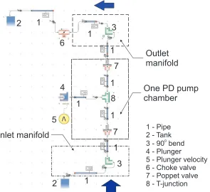
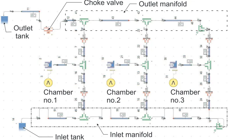
Figure 1 shows the Flowmaster model of a single cylinder pump from which the triplex pump of Figure 2 was created. The legend in Figure 1 explains the items comprising the model. Water flows from the left tank through the pump chamber to the right tank, performing first the suction stroke and then the delivery stroke. During the suction stroke the chamber (highlighted in yellow) is filled as the plunger moves backwards and leaves the displacement volume for the water to fill. The inlet and outlet valves are modelled as poppet valves for which the analyst has to specify the valve seat area, the valve disk area, the spring preload, spring rate and the valve loss coefficient as a function of the valve lift normalised by the max lift value. The valve loss coefficient is essential to calculate the pressure drop across the valve against the valve lift. The estimation of the valve loss coefficient was carried out by means of 3D-CFD simulation and will be discussed in the next paragraph. Obviously the layout of the 1D system was decided in order to keep it as close as possible to the experimental apparatus which will be discussed in later in this paper.
1
2
3
4
5
6
7
1
1
1
7
1
1
3
1
1
2
8
1 - Pipe 2 - Tank 3 - 90 bend 4 - Plunger
5 - Plunger velocity 6 - Choke valve 7 - Poppet valve 8 - T-junction
0
Inlet manifold
One PD pump
chamber
[image:4.595.158.453.138.408.2]Outlet
manifold
[image:4.595.52.550.460.501.2]Figure 1. Simplex (Single cylinder) pump using lumped parameter model.
Table 1. Reciprocating motion parameters
Crank radius (r) [m] Connecting rod length (l) [m] Crank angular velocity (ω) [rad/s] Con-rod/crank radius (µ) [-]
0.02 0.105 45.93 5.25
this paper. The plunger velocity was imposed by providing the code with the velocity-time function shown in Figure 3 which was built by means of equation 1 where r,ωand µ are the crankshaft radius respectively. These angular velocity and the connecting rod/crankshaft radius ratio, these parameters are provided in Table 1. The angular velocity was considered constant throughout the reference tests. The reader should note that the three cylinder model of Figure 2 is an extended version of the single cylinder model where the suction and delivery pipe of the second and third chamber were connected to the same manifolds of chamber 1. The velocities of plungers 2 and 3 have a phase offset to plunger 1 of 240◦and 120◦. Apart from the plunger velocity, the boundary conditions were set as the static pressure in the inlet and outlet tank where the value was decided by the water level and the height of the base.
v(t) =rω
sin(ωt) +
sin2(ωt)
2
q
µ2−sin2(ωt)
(1)
The results obtained by the one-cylinder model will be discussed as well as those obtained with the three cylinders model which will be compared to the experimental tests. The analysis was incompressible and transient and the execution time on an IntelR XEONR CPU E5-1650 v3 @ 3.5 GHz processor was 30 seconds to 1.5 minutes for the single chamber model and the three chamber model respectively. The time step chosen was 1.368·10−4s which corresponds to 0.1% of the time needed to complete one pumping cycle at the specified velocity. It was chosen to run 10 pumping cycles for an overall simulation time of 0.1368 seconds.
3 CFD Model
Inlet tank
Outlet
tank
Choke valve
Chamber
no.1
Chamber
no.2
Chamber
no.3
Inlet manifold
[image:5.595.107.503.140.382.2]Outlet manifold
Figure 2. Triplex (three-cylinder) pump using lumped parameter model.
-1.50 -1.00 -0.50 0.00 0.50 1.00 1.50
0 50 100 150 200 250 300 350
V
elocity
[
m/s]
Crank rotation [˚]
[image:5.595.161.442.426.605.2]Plunger 1 velocity Plunger 2 velocity Plunger 2 velocity
Figure 3. Plunger velocity (function of the crankshaft parameters), plunger 2 and 3 have an offset of 240◦and 120◦respectively.
Table 2. Boundary conditions for the two set of tests
Inlet boundary conditions
Outlet boundary
conditions Monitor function Suction valve K
estimation simulations
Mass flow rate fixed
on the pump suction manifold
Static pressure (0 Pa) on the plunger top surface
∆P between inlet and outlet Discharge valve K
estimation simulations
Mass flow rate fixed on the plunger top surface
Static pressure (0Pa) fixed on the pump discharge manifold
∆P between inlet and outlet
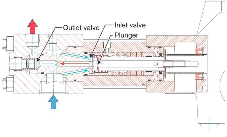
[image:5.595.55.548.657.738.2]Inlet valve
Outlet valve
[image:6.595.119.502.146.378.2]Plunger
Figure 4. Internal geometry of the PD pump used in the experimental and numerical analysis
The valve loss coefficient defines the pressure drop across the valve with respect to the valve lift, it is normalised by the dynamic pressure upstream of the valve as shown in equation 2.
K= 1∆P
2ρV2
(2)
Each of the two models presented in Table 2 were modified and launched six times in order to have six evaluations of the pressure drop across the valves for six valve lift values. The∆P entered in equation 2 gave the loss coefficient for six
valve lifts from 0 mm to the valve maximum opening. The values of the loss coefficient were arranged in a piecewise linear function against the valve lift ratio (li f t/li f tMAX), this function was input into the Flowmaster model of the valve.
It is important to note that the flow velocity upstream of the valve specified in equation 2, is a function of the mass flow rate chosen as the boundary condition (Table 2) which, in real conditions, is proportional and therefore fixed by the plunger velocity and the pipe diameter upstream the valve. This means that the CFD model has to be consistent with the Flowmaster model to make sure that the loss coefficient K is normalised correctly. However, as long as the analysis is consistent, only one mass flow rate is needed for each valve lift as the normalization of the loss coefficient makes it independent from the mass flow rate. As the operations to modify the valve lift and re-evaluate the pressure drop were simple, the authors decided to utilise ANSYS Workbench in conjunction with ProEngineer Creo (as CAD software) to automate them; changing the valve lift , recreate the model and solve it. The workflow is shown in Figure 5 which describes the operation performed by ANSYS Workbench once the valve lift was parametrised. The mass flow rate chosen for the 6 steady state simulations was 10% of the maximum mass flow rate at the chosen plunger maximum velocity.
3.1 3.1 CFD details, settings and results
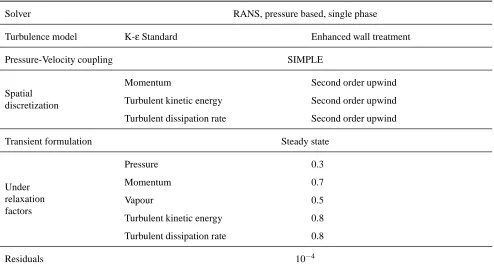
The fluid volumes were meshed by making use of tetrahedral cells. The size of the cells was decided by a mesh sensitivity test which was carried out previous to the analysis. For this purpose three meshes of different size were tested under the same conditions. The smallest one which provided the solution insensitive to the size was chosen for the analysis. The overall number of cells was approximately one million. Two layers of prismatic cells were put on the walls to simulate the behaviour of the boundary layer and support the action of the near wall treatment algorithm. A K-εturbulence model was chosen as it provided better convergence over the K-εbut the ”enhanced wall treatment” [14] was utilised to correct the wall function where the y+ values were outside the optimum range for the chosen turbulence model. The general settings chosen for the solver are summarised in Table 3.
Valve lift = initial value
Solid assembly preparation (Creo)
Fluid volume extraction (ANSYS geometry)
Fluid volume mesh (ANSYS Mesher)
CFD solution (ANSYS Fluent)
Valve lift = next value
Calculation of the pressure drop across the valve
[image:7.595.129.484.134.403.2]Store data
Figure 5. Workflow of the operations executed by ANSYS Workbench for the discrete evaluation of the loss coefficient K
Table 3. Solver settings summary
Solver RANS, pressure based, single phase Turbulence model K-εStandard Enhanced wall treatment
Pressure-Velocity coupling SIMPLE
Spatial discretization
Momentum Second order upwind
Turbulent kinetic energy Second order upwind Turbulent dissipation rate Second order upwind
Transient formulation Steady state
Under relaxation factors
Pressure 0.3
Momentum 0.7
Vapour 0.5
Turbulent kinetic energy 0.8 Turbulent dissipation rate 0.8
Residuals 10−4
[image:7.595.56.550.461.730.2]1 10 100 1000 10000 100000
0 0.2 0.4 0.6 0.8 1
K [
-]
Valve opening ratio [-]
[image:8.595.143.453.142.337.2]Outlet valve opening Inlet valve opening
Figure 6. Inlet and Outlet valve loss coefficient, this trend was input as piecewise linear function in the Flowmaster model of the valve.
WATER TANK CONTROL PANEL
EL. MOTOR
PD PUMP
[image:8.595.54.279.383.525.2]PNEUMATIC RAGULATOR
Figure 7. Skid assembly with major components
PNEUMATIC VALVE PD PUMP
POWER END
FLUID END
Figure 8. PD pump assembly with regulating pneumatic valve
Figure 9. Test rig assembly
4 Experimental setup
In this section the experimental setup will be presented. The test rig was assembled on a single skid. The main compo-nents are annotated in Figure 9. Figure 10 summarises the important parameters associated with the chosen PD pump [15]. The device was driven by a 37 kW electric motor [16] which was designed to operate up to 1800 rpm. The pump operating speed was regulated using a variable frequency controller.
4.1 Pump operation
The pump operated in a closed loop system which circulated water from the water tank in a similar way as described in paragraph 2. The only difference is that, in the real apparatus the suction tank and the delivery tank were actually the same item. According to the manufacturer specification the pump needed to be supplied with a constant source of clean cold water, therefore, a 500 litre capacity stainless steel water tank was chosen and mounted onto the pump skid directly above the pump. The water tank was fitted with an inlet point for the initial filling from an external source. An inlet float valve was also included to prevent over filling.
The pipework included a selection of valves and hoses to connect the tank to the pump, the pump to the solenoid valve and the solenoid valve back to the tank. A manually operated drain valve was included to allow the system to be emptied when required. A manually operated ball valve was also included to isolate the pump inlet from the tank. This valve was fitted with a limit switch to prevent the pump from operating in a closed valve condition.
[image:8.595.303.530.383.525.2]HPS 400 Pump specification
Plunger Diameter (m) 0.022
Number of Plungers 3
Stroke (m) 0.045
Operating speed (rpm) 789 Gearbox ratio (-) 2.28:1 Displaced volume (m3) 1.7·10−5
[image:9.595.73.473.144.292.2]Maximum operating pressure (MPa) 40 Maximum flow rate (l/min) 41 Maximum power requirement (kW) 30
Figure 10. Essential operating parameters from the test pump [15]
Variable Frequency Drive Electric Motor
Water Tank Ball
Valve
Solenoind Valve Pressure
relief valve PS PS PS
FS RS
PS
outlet
inlet
PSL
Pressure sensor - discharge
PS Range:0-600bar(a)
Response time: 1ms
Pressure sensor - low
PSL Range:0-1.6bar(a)
Response time: 1ms
Rotational encoder
RS Sensor type: Digital counter
Flow rate meter
FL Range: 0-41l/min
Accuracy: 0.1%
Figure 11. Test rig schematics and essential sensor information
Drive (VFD) [17] knob on the system control panel. The rotation of the driveshaft was converted into the linear motion of the plungers via the crankshaft. The group comprising of the motor, gear box and crankshaft is usually referred to as the ”power end” and it is indicated under the same label in Figure 9. The parts of the pump which process directly the working fluid (plunger, valves, pump external case and pipes) are usually referred to as ”fluid end” and are shown in Figure 9. The pressure head of the tank ensured that there was no cavitation inside the pump. A solenoid choke valve was placed downstream the pump as shown in Figure 11. The valve was driven by an electro-pneumatic system which was manually controlled by the operator on the control panel. The operator gradually shut-off the valve to pressurise the outlet line to the pressure value required for the tests. Downstream of the choke valve the pressure was approximately equal to the tank pressure. The fluid was, then, led back to the tank.
4.2 Instrumentation and data acquisition 4.2.1 Speed control
The motor speed control was achieved in two different ways. The first one, already mentioned, was the manual action on the system control panel. The second was the addition of a ModBus device on the VFD that enabled the control via Ethernet connection. The advantage of this method was not only the ability to control the device remotely but also to operate it by using a PC interface with the unit that enables the design of speed adjustments and feedback control. For the purpose of the experiments carried out and discussed in this paper, the first control method was adequate to satisfy the control requirements. 4.2.2 Pressure control
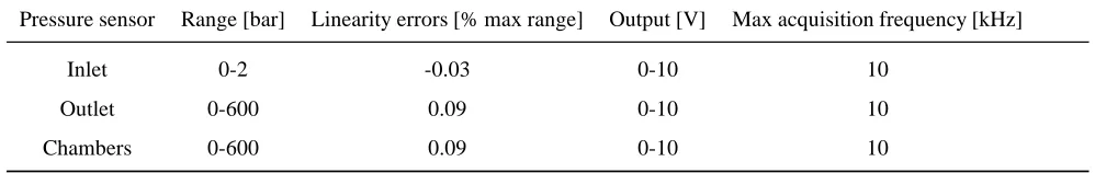
[image:9.595.111.471.329.506.2]Table 4. Pressure sensor characteristics summary
Pressure sensor Range [bar] Linearity errors [% max range] Output [V] Max acquisition frequency [kHz]
Inlet 0-2 -0.03 0-10 10
Outlet 0-600 0.09 0-10 10
Chambers 0-600 0.09 0-10 10
by varying the air pressure acting on the valve on the electro-pneumatic actuator moving the valve. The valve control was manual and included in the control panel, where a current/pressure convertor regulated the air pressure acting on the valve via a 4-20mA signal.
4.2.3 Pressure sensors
Five pressure sensors [18] were installed throughout the system; three of them were placed on the top of the pump, acquiring the pressure in each of the pump chambers, an inlet and outlet pressure sensor was also placed on the inlet and outlet pipe to monitor the suction and delivery pressure. As the inlet pressure sensor was never subjected to high pressure during the pumping cycle its characteristics and specifications were chosen differently from the other sensors. The differences are described in Table 4.
4.2.4 Speed sensor
Using a reflective tape placed on the crankshaft and a static infrared sensor [19] pointed at it, the initial angular position of the crankshaft was fixed. The reflective tape was placed on the crankshaft in the position which corresponded to the Top Dead Centre of plunger number 1. The position of plungers number 2 and 3 were also proportional to the crankshaft position. The drive-shaft speed could then be determined based on the number of pulses per minute measured by the sensor which output a digital counter signal every time the reflective tape passed in front of the sensor during the rotation.
4.2.5 Flow sensor
A flow meter on the pump inlet was also included. This was a stainless steel Pelton wheel turbine type with 1/2” inlet and outlet connections. The output from the flow meter was fed to a digital display unit that was mounted on the pump control panel. A 4-20mA output signal could then be taken from the display unit for manipulation and recording by a data acquisition system. The flow meter installed operated with an accuracy of 2% for the top 90% of the range.
4.2.6 DAQ
The external device handling and manipulating the signals (pressures, flow rate and speed) was a USB National Instru-ment DAQ [20] which was connected to a PC where Labview was installed, for this purpose a Labview specific programme was written. The acquisition frequency was set into the programme and fixed at 10 kHz.
5 Results and discussion
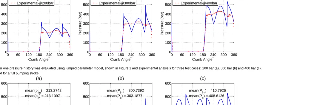
In Figure 13 three of the performed reference tests are presented. Overall outlet pressure in the discharge manifold was evaluated during one pumping cycle (360◦).The oscillation of the signal around the mean value is evidence of the interaction of the three chambers which takes place in the outlet manifold. One may assume that the simplified lumped parameter model accurately accounts the pressure frequencies but overestimates its amplitudes.
0 60 120 180 240 300 360 0 100 200 300 400 500 600
(a)
Pressure (bar)Crank Angle°
0 60 120 180 240 300 360 0 100 200 300 400 500 600
(b)
Pressure (bar)Crank Angle°
0 60 120 180 240 300 360 0 100 200 300 400 500 600
(c)
Pressure (bar) [image:11.595.59.645.73.249.2]Crank Angle° Flowmaster@200bar Experimental@200bar Flowmaster@300bar Experimental@300bar Flowmaster@400bar Experimental@400bar
Figure 12. Chamber one pressure history was evaluated using lumped parameter model, shown in Figure 1 and experimental analysis for three test cases: 200 bar (a), 300 bar (b) and 400 bar (c). Tests were performed for a full pumping stroke.
0 60 120 180 240 300 360 100 200 300 400 500 600
(a)
Pressure (bar)Crank Angle° mean(p
e) = 213.1097
mean(p
fm) = 213.2742
Flowmaster@200bar Experimental@200bar
0 60 120 180 240 300 360 100 200 300 400 500 600
(b)
Pressure (bar)Crank Angle° mean(P
e) = 303.1877
mean(P
fm) = 300.7392
Flowmaster@300bar Experimental@300bar
0 60 120 180 240 300 360 100 200 300 400 500 600
(c)
Pressure (bar)Crank Angle° mean(P
e) = 408.6126
mean(P
fm) = 410.7926
Flowmaster@400bar Experimental@400bar
Figure 13. Experimental evaluation of pressure field inside the common outlet manifold chamber in a triplex pump vs numerical evaluation of common manifold chamber, illustrated in Figure 2, using lumped parameter model. Three reference test were conducted at 200 bar (a), 300 bar (b) and 400 bar (c). The mean values of experimental and numerical pressures are displayed aspeandpf m
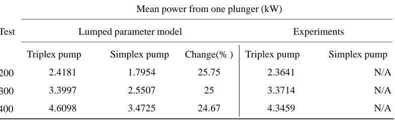
[image:11.595.77.645.284.484.2]Table 5. Summary of the power consumption from single plunger. Lumped parameter model evaluated single cylinder consumption in triplex (three-cylinder) pump and simplex (one-cylinder) pump. Experimental data was only able to evaluate power consumption of single cylinder in triplex pump. Future studies will look into experimental power analysis of a single cylinder in simplex pump.
Mean power from one plunger (kW)
Test Lumped parameter model Experiments
Triplex pump Simplex pump Change(% ) Triplex pump Simplex pump
200 2.4181 1.7954 25.75 2.3641 N/A
300 3.3997 2.5507 25 3.3714 N/A
400 4.6098 3.4725 24.67 4.3459 N/A
5.1 Power evaluation
Application of an accurate lumped parameter model of a complete multi-cylinder pump is justified by the need for estimating the performance of an entire pump. The interference among the chambers, makes the individual chamber analysis insufficiently accurate for this purpose.
For instance, the lumped parameter model could estimate the power loss in the cylinders interaction. Figure 14 shows the power resistance calculated on the plunger for the three reference tests. The experimental data was evaluated by appraising plunger in chamber one. By examining three test cases it is clear that power requirement in one plunger in triplex pump is higher than in simplex pump (one cylinder) by approximately 25%, shown in Table 5 (third vs second column). It can be assumed that a single cylinder pump would need less than the same cylinder in a triplex pump of the same kind, or, conversely a triplex pump would need more than three times the power needed by each separate chamber. Power difference is constituted by the power loss in the interaction.
Engineering rationale for this phenomenon is that at the beginning of the delivery stroke each plunger has to work against the high pressure created in the outlet manifold (generated by the delivery stroke of other chambers). The novelty provided by the analysis methodology described in this section is the quantification of this power gap which can be examined in ‘Change(%)’ column of Table 5.
Validity of the lumped parameter model is clearly stated by comparing ‘Triplex pump’ columns from experimental and numerical analysis shown in Table 5. Power consumption values are remarkably close (approximately 2% differentiation) for each of the test cases indicating the high accuracy of the computational model.
In Figure 15 computational lumped parameter model is presented. Each of the test cases was performed at different outlet pressure which is directly proportional to the pump load factor. In each of the three test cases two main operating states were analysed; in the first, cylinder one was analysed in a triplex pump and in the second, the same cylinder was evaluated in simplex pump. The hatched area presents the power loss that is taking place in triplex pump due to cylinder interaction.
It is true that, for an absolute validation of the data in Table 5, the single cylinder lumped parameter model should be compared to a single cylinder experimental test. Experimental data is still unavailable as shown Table 5. The authors are currently working to complete the experimental campaign despite difficulties of isolating two of the three chambers in a triplex test pump. From computational lumped parameter model it can be seen, in Figure 15, that the estimation of the difference in power consumption made above is approximately 25%. The figures, in fact, show the numerical comparison between the three chambers and the single chamber lumped parameters model throughout the reference tests. The area in figure
5.2 Discussion of a multi-cylinder PD pump model
Multi-cylinder pump section has demonstrated that one of the major challenges present in modelling of PD pumps is the interaction between cylinders. Using 1D-CFD software it was proved that problem identification and performance changes in hydraulic systems are attainable using combination of different commercial softwares. High-fidelity CFD codes show effectiveness in solving simplex pump designs. Multi-cylinder models are not affordable in industrial applications due to the high computational time. Lumped parameter model are ideal for high level system layout with multiple individual units and elements such as pumps, safety valves, hoses, etc. Synergy of two systems provides optimal solution that takes into account high level and in-depth analysis.
0 60 120 180 240 300 360 0 5 10 15 20
(a)
Power (kW)Crank Angle° mean(P
e) = 2.3641
mean(Pfm) = 1.7954 Flowmaster power Experimental power
0 60 120 180 240 300 360 0 5 10 15 20
(b)
Power (kW)Crank Angle° mean(P
e) = 3.3714
mean(Pfm) = 2.5507 Experimental power Flowmaster power
0 60 120 180 240 300 360 0 5 10 15 20
(c)
Power (kW)Crank Angle° mean(P
e) = 4.3459
[image:13.595.79.646.44.244.2]mean(Pfm) = 3.4725 Experimental power Flowmaster power
Figure 14. Experimental evaluation of one chamber in a triplex pump vs numerical evaluation of one chamber in a simplex pump (shown in Figure 2). Power consumption was measured and calculated at 200 bar (a), 300 bar (b) and 400 bar (c). Experimental and numerical mean power consumptions values are displayed forPeandPf mrespectively.
0 60 120 180 240 300 360
0 2 4 6 8 10 12 14 16 18 20 Power (kW)
Crank Angle° mean(P
fm1) = 3.3678 mean(P
fm3) = 3.8612 1 cylinder in triplex (FM) 1 cylinder in single (FM)
0 60 120 180 240 300 360
0 2 4 6 8 10 12 14 16 18 20 Power (kW)
Crank Angle° mean(P
fm1) = 4.8123 mean(P
fm3) = 5.4369 1 cylinder in triplex (FM) 1 cylinder in single (FM)
0 60 120 180 240 300 360
0 2 4 6 8 10 12 14 16 18 20 Power (kW)
Crank Angle° mean(P
fm1) = 6.5583 mean(P
fm3) = 7.4058 1 cylinder in triplex (FM) 1 cylinder in single (FM)
[image:13.595.77.657.270.511.2]This research has illustrated how application of commercial software can be used and customized to answer design requirements. Site variation can be overcome by in-depth analysis, standardisation and implementation of engineering solutions to site.
References
[1] Iannetti, A., Stickland, M. T., and Dempster, W. M., 2014. “A computational fluid dynamics model to evaluate the inlet stroke performance of a positive displacement reciprocating plunger pump”. Proceedings of the Institution of
Mechanical Engineers, Part A: Journal of Power and Energy. URL.
[2] Sloesen, J., and Kuenen, J., 2011. “Pd pumps, the modern solution for pumping high density tailings”. URL.
[3] Deepak, C., Shajahan, M., Atmanand, M., Annamalai, K., Jeyamani, R., Ravindran, M., Schulte, E., Handschuh, R., Panthel, J., Grebe, H., et al., 2001. “Developmental tests on the underwater mining system using flexible riser concept”. In Fourth ISOPE Ocean Mining Symposium, International Society of Offshore and Polar Engineers. URL.
[4] Clark, C. R., Carter, G. L., et al., 1973. “Mud displacement with cement slurries”. Journal of Petroleum Technology, 25(07), pp. 775–783. URL.
[5] De Pater, C., Beugelsdijk, L., et al., 2005. “Experiments and numerical simulation of hydraulic fracturing in naturally fractured rock”. In Alaska Rocks 2005, The 40th US Symposium on Rock Mechanics (USRMS), American Rock Mechanics Association. URL.
[6] Manring, N. D., 2000. “The discharge flow ripple of an axial-piston swash-plate type hydrostatic pump”. Journal of
dynamic systems, measurement, and control, 122(2), pp. 263–268. URL.
[7] Zhang, X., Cho, J., Nair, S., and Manring, N., 2001. “New swash plate damping model for hydraulic axial-piston pump”. Journal of Dynamic Systems, Measurement, and Control, 123(3), pp. 463–470. URL.
[8] Dash, A., and Cudworth, G., 1998. “Therapeutic applications of implantable drug delivery systems”. Journal of
pharmacological and toxicological methods, 40(1), pp. 1–12. URL.
[9] Johnston, D. N., 1991. “Numerical modelling of reciprocating pumps with self-acting valves”. Proceedings of the
Institution of Mechanical Engineers, Part I: Journal of Systems and Control Engineering, 205(2), pp. 87–96. URL.
[10] K. A. Edge, O.P. Boston, S Xiao, M.J. Longvill, C.R. Burrows, 1997. “Pressure pulsation in reciprocating pump piping systems: Part2”.
[11] Edge, KA and Boston, OP and Xiao, KCS and Longvill, KCMJ and Burrows, KCCR, 1997. “Pressure pulsations in reciprocating pump piping systems part 2: Experimental investigations and model validation”. Proceedings of
the Institution of Mechanical Engineers, Part I: Journal of Systems and Control Engineering, 211(3), pp. 239–250.
DOI:10.1243/0959651971539777.
[12] Iannetti, A., Stickland, M. T., and Dempster, W. M., 2016. “A cfd and experimental study on cavitation in positive displacement pumps: Benefits and drawbacks of the fullcavitation model”. Engineering Applications of Computational
Fluid Mechanics, 10(1), pp. 57–71. DOI:10.1080/19942060.2015.1110535.
[13] Miller, D. S., 1990. Internal flow system. BHRA. ISBN: 978-0956200204.
[14] ANSYS, 2011. ANSYS Fluent Theory Guide,s vol. 15317, no. November. ANSYS Inc.
[15] Hughes Pumps, 2015. Hps400 high pressure triplex pump - technical paper (online). Accessed: 08 Jun 2015. URL. [16] Brook Crompton, 2015. W cast iron motors - technical paper (online). Accessed: 28 Jan 2016. URL.
[17] ABB, 2015. Abb industrial drives - technical paper (online). Accessed: 08 Jun 2015. URL.
[18] HYDROTECHNIK, 2016. Hysense pr 400/410 pressure sensors - technical paper (online). Accessed: 24 May 2016. URL.
[19] Honeywell Sensing and Control, 2016. Hoa series infrared reflective sensor - technical paper (online). Accessed: 22 Jan 2016. URL.

![Figure 10.Essential operating parameters from the test pump [15]](https://thumb-us.123doks.com/thumbv2/123dok_us/1462894.98958/9.595.111.471.329.506/figure-essential-operating-parameters-test-pump.webp)