Sensitivity analysis using risk measures

City, University of London Institutional Repository

Citation

:

measures. Risk Analysis: an international journal, 36(1), pp. 30-48. doi: 10.1111/risa.12434

This is the accepted version of the paper.

This version of the publication may differ from the final published

version.

Permanent repository link:

Link to published version

:

Copyright and reuse:

City Research Online aims to make research

outputs of City, University of London available to a wider audience.

Copyright and Moral Rights remain with the author(s) and/or copyright

holders. URLs from City Research Online may be freely distributed and

linked to.

City Research Online: http://openaccess.city.ac.uk/ [email protected]

Sensitivity analysis using risk measures

Andreas Tsanakas †1 _{and Pietro Millossovich}‡1

1_{Faculty of Actuarial Science and Insurance, Cass Business School, City University}

London

∗_{Accepted for publication in}

Risk Analysis: An International Journal. We thank two referees for constructive

feedback. Earlier versions have been presented at the 17th_{International Congress on Insurance: Mathematics and}

Economics, the 6th_{International Conference of the ERCIM WG on Computational and Methodological Statistics,}

the 6th _{International Conference on Mathematical and Statistical Methods for Actuarial Sciences and Finance,}

theFISC 2014 Conference, and at research seminars in the Department of Mathematics, ETH Zurich, the Faculty

of Economics, KU Leuven, and the Department of Mathematics and Statistics, University of Montreal. We thank

Jens Perch Nielsen, Mar´ıa Dolores Miranda-Mart´ınez and Mario W¨uthrich for helpful discussions.

Abstract: In a quantitative model with uncertain inputs, the uncertainty of the output can be summarized by a risk measure. We propose a sensitivity analysis method based on derivatives of the output risk measure, in the direction of model inputs. This produces a global sensitivity measure, explicitly linking sensitivity and uncertainty analyses. We focus on the case of distortion risk measures, defined as weighted averages of output percentiles, and prove a representation of the sensitivity measure that can be evaluated on a Monte-Carlo sample, as a weighted average of gradients over the input space. When the analytical model is unknown or hard to work with, non-parametric techniques are used for gradient estimation. This process is demonstrated through the example of a non-linear insurance loss model. Furthermore, the proposed framework is extended in order to measure sensitivity to constant model parameters, uncertain statistical parameters, and random factors driving dependence between model inputs.

1

INTRODUCTION

Sensitivity analysis, alongside uncertainty analysis, is an activity of fundamental importance to

risk analysts, especially in the presence of complex computational models with uncertain inputs.

Reasons for performing sensitivity analyses include the need to rank the relative importance of

input variables, to uncover relations between inputs and outputs in complex models, to perform

quality assurance and reasonableness checks, and to identify areas of investigation and refinement

in the model(1–5). Sensitivity analysis comprises a wide range of methodologies, with global

sensitivity approaches, reflecting the model behaviour over the whole of the input range(3,5,6),

becoming the norm in recent years. Such methods have seen wide application in risk analysis;

indicatively we mention safety assessment for nuclear waste disposal(7), food safety(2), microbial

risk assessment(8), and climate change modelling(9).

Global sensitivity approaches are concerned with “how uncertainty in the output of a model

[...] can be apportioned to different sources of uncertainty in the model input”(5). In

moment-based global sensitivity analyses(3,5)_{, the variance of outputs is typically apportioned to}

contri-butions of input variable volatilities. While such analyses are revealing, it is known that using

the variance as a measure of variability can lead to violations of standard dominance

require-ments(10). Furthermore, application of variance-based sensitivity methods becomes involved

when inputs are correlated. Such considerations have motivated the design of moment-free

sen-sitivity analyses(6,11–13), which reflect the difference between the conditional and unconditional

output density via a distance measure.

We consider models where a number of uncertainmodel inputs are mapped to a singleoutput

of interest via a known model function. Both inputs and outputs are observable. Uncertainty

analysis allows determination of the output’s probability distribution, e.g. via Monte-Carlo

a statistical functional that maps a random variable to a real number(14,15). Moments such as

the mean and variance are examples of risk measures. A flexible and widely applicable class

aredistortion risk measures(14,16–18)_{, arising as weighted averages of percentiles. The weighting}

function encodes preferences, in the sense that particular areas of the output probability

dis-tribution, corresponding to states of interest, can be focused on. The class of distortion risk

measures includes most coherent risk measures(19) _{of interest. The sensitivity of optimization}

problems that involve such risk measures is studied in Ref.(20).

We propose a sensitivity analysis method that directly links to uncertainty analysis through

the use of risk measures. Specifically, we argue in favor of measuring sensitivity by adirectional

derivative of the risk measure applied on the output, in the direction of model inputs. The

result-ing sensitivity measure satisfies the desirable properties of Saltelli(3)_{. In particular, it is global,}

in the sense that it is generated by the weighted average of local sensitivities over the whole of

the input space. The proposed method is general enough to cope with measurement of

sensitiv-ity to various types of variables, such as (i) uncertain model inputs; (ii) statistical parameters

of the distributions of inputs that are subject to uncertainty; (iii) known structural parameters;

(iv) common factors driving dependence between inputs. The calculation of sensitivities can

be carried out on a single Monte-Carlo sample of model inputs and outputs – computational

speed can be further improved for high-dimensional models if information on the hierarchical

(multi-level) construction of the model functions is available. While the method is in principle

applicable to any type of risk measure (including moment-based ones), we focus on the case

where the output distribution is summarized by a distortion risk measure.

In Section 2, the sensitivity to each model input is defined as the derivative of the risk

mea-sure applied on the output, with respect to the scale of a random shock applied to that model

input. The sensitivity thus is a directional derivative, which makes the sensitivity measure a

to non-linear models. For distortion risk measures, an explicit formula for the sensitivity

mea-sure is derived, extending existing results(24,25). The resulting sensitivity is expressed as an

expectation involving the random shock, the corresponding gradient of the model function, and

scenario weights generated by the risk measure. Thus the sensitivity measure reflects

informa-tion about the statistical behaviour of the model inputs, the shape of the model funcinforma-tion, and

preferences. There is flexibility in relation to the shock chosen and we particularly focus on

shocks that produce proportional changes to model inputs.

The formal properties of the sensitivity measure are discussed in Section 2.3, where its

relation to other sensitivity analysis approaches is also discussed. Conceptual parallels are

identified between the properties our sensitivity measure and the concerns of standard methods

such as Regional Sensitivity Analysis(26)_{, elementary effects}(27)_{, variance-based sensitivity}(3,5)

and moment-free sensitivity(6).

In Section 3, the implementation and communication of the sensitivity analysis is

demon-strated, using the example of a non-linear insurance loss model. The analysis is performed on a

Monte-Carlo sample of the portfolios. We do not calculate the gradient of the model function

analytically, but instead put ourselves in the shoes of an analyst or reviewer who has access to

the simulated samples of the model inputs and output only, but no direct access to the model’s

analytical form. This corresponds to practical situations, where there is limited access to model

documentation and/or the model is too complicated to make analytical calculations

appeal-ing. Then, the gradients of the model are estimated numerically from the simulated sample,

borrowing tools from non-parametric statistics, in particular local linear regression(28,29).

In Section 4, the proposed methods are extended to the measurement of the sensitivity to

parameters and the dependence structure. For this purpose, known model parameters, treated

as degenerate model inputs, are artificially randomized. Sensitivity to statistical parameters

average of distributions (a mixture) over possible parameter values. We express an model input

subject to parameter uncertainty as a function of two independent random variables, representing

stochastic and parameter uncertainty respectively. The sensitivity to each of the two elements

is then calculated.

Correlation and, more broadly, dependence between inputs is understood as a major driver

of output variability(12)_{, see also Ref.}(30) _{for an extensive treatment. Many commonly used}

dependence structures can be expressed via conditional independence, given a number of latent

or observable common factors. We proceed by measuring sensitivity to those common factors.

This entails expressing the vector of dependent model inputs as a function of a vector of

in-dependent idiosyncratic and common factors; we present a probability transform that enables

such a decomposition.

Brief conclusions are stated in Section 5; formal statements of results and proofs are given

in the Appendix.

2

SENSITIVITY ANALYSIS

2.1 Preliminaries

For the purposes of this paper, a model consists of three elements: a vector X of inputs, a

functiong, and an output variableY =g(X). We call the elements of X model inputs. Model

inputs are uncertain; they can be subject to both epistemic uncertainty and stochastic variability.

Uncertainty is modelled by consideringX a random vector taking values in an open convex set

X ⊂Rd _{and with joint probability distribution F. We call g :X →}R_{the model function and}

Y theoutput. For simplicity, we will typically assume that that high values ofY correspond to

undesirable states of the world, for instance in the case that Y stands for a financial loss.

assume here and in the sequel that distributions are strictly increasing and continuous, though

the results in this paper do not require such assumptions. Then, for u ∈ (0,1), the inverse

F_Y−1(u) gives the 100uth _{percentile of Y. We calloutput rank the uniformly distributed random}

variableUY =FY(Y), such that Y =FY−1(UY).1

A risk measure is a functional ρ mapping random variables to the real line. For example,

ρ(Y) =E_{(Y) andρ(Y) =}V_{(Y), the mean and the variance, are risk measures. Here we consider}

the class of distortion risk measures, defined as weighted averages of percentiles. Consider a

non-negativeweight function ζ on [0,1] withR1

0 ζ(u)du= 1. The functionζ reflects preferences,

in the sense that it allows assigning a higher weight to output ranks corresponding to (generally

undesirable) states of the world that are of specific interest. The distortion risk measure, as

applied to the random variable Y, is given by the relation

ρ(Y) = Z 1

0

F_Y−1(u)ζ(u)du=E _{Y ζ(UY)}

. (2.1)

To distinguish the risk measureρas an abstract functional, from the valueρ(Y), we call the latter

therisk summary ofY. The right-hand-side of equation (2.1) shows that the risk summary ofY

may also be represented as its expected value, subject to a re-weighting of probabilities effected

by ζ (note that E_{(ζ(UY)) = 1). Distortion risk measures were introduced in the actuarial} literature by Wang et al.(16)_{. Such risk measures have found wide application in insurance}

pricing, financial risk management and risk analysis(14,17,18).

This class of risk measures is fairly flexible and admits commonly used measures as special

cases. The constant weight functionζ(u) = 1 gives the mean. The 100pth percentile, F_Y−1(p), is derived for a trivial weight functionζ(u), with a mass concentrated atp, such that a weight of 1 is

1_{For a general distributionF}

Y, the definitions are easily extended. The generalized inverseFY−1(u) = inf{y:

P₍Y ≤ y) ≥ u} is defined. There still exists a random variable UY such that Y = FY−1(UY), but it is no

longer unique. A simple explicit construction of the output rankUY is given by the generalized distributional

attached toF_Y−1(p) and a weight of zero to all other percentiles. In finance,F_Y−1(p) corresponds to the Value-at-Risk measure, denoted by VaRp. Let 1A be the indicator function of an event

(or set) A, taking value 1 when the event is true and zero otherwise. Then, ζ(u) = ₁₋1_p1_{u>p}, applying a constant weight to percentiles more extreme than the 100pth, gives rise to Tail-Value-at-Risk (TVaR), TVaRp(Y) = ₁₋1_pR_p1F_Y−1(u)du = E(Y|Y > F_Y−1(p)), with the second

equality holding whenFY is continuous. The VaR and TVaR risk measures are extensively used

in financial risk management(32), while other weighting functions considering the whole of the

output distribution are available(18,30). When the function ζ is non-decreasing (as in the case

of TVaR), the corresponding risk measure ρ is a convex functional, thus satisfying the axioms

of coherent risk measures(19). For coherent risk measures, inconsistent orderings of probability

distributions, such as those identified by Cox(10)_{, are avoided.}

It is not obvious how to best choose a risk measure. Sometimes, particular risk measures are

prescribed by regulation. For example, in an insurance context, capital requirements under the

European Solvency II regime are calculated by VaR0.995(33), while under the Swiss Solvency Test

a TVaR0.99measure is used(34). The choice of these measures is dictated by their regulatory use,

as they both are simple and focus on extreme adverse events. For internal use, which is related

to sensitivity analysis, one need not restrict to those or indeed to any single risk measure. The

choice of risk measure will be discussed further through Examples 1 and 2.

2.2 Sensitivity measures

We measure the sensitivity of the output risk summary to an individual model input, by stressing

that model input with a random shock. Specifically, consider a random variable Z and ǫ > 0.

Denote by ei the vector in Rd with 1 in the ith position and 0 elsewhere. Then, the vector of

model inputs with a shock ǫZ applied to the ith element is written as X+ǫZei. Additionally,

The application of the shock ǫZ corresponds to a change in the distribution of the random

variable Xi (and more generally the random vectorX), effected by adding to it another source

of uncertainty. The selection of Z depends on the purpose of the sensitivity analysis. If one

wants to study for example the impact of increasing the variability ofXi, thenZ can be chosen

to have a mean of zero. It will be seen below that it is possible without loss of generality to

restrict attention to shocksZthat are functions of the random vectorX, such thatZandXi will

generally be dependent random variables. We note that this way of changing the distribution

of the inputs, by perturbing the random inputs directly, is distinct from a perturbation of the

probability distribution itself as practised in Bayesian(35) and robust(36) statistics.

The sensitivity to the shock Z is now defined as the derivative of the risk summary of the

stressed outputρ(g(X+ǫZei)) with respect toǫ, evaluated atǫ= 0.2 Hence, it is a directional

derivative in the direction ofZ. Such derivatives have been considered in finance, where generally

only linear model functions are considered(21–23), while non-linear models are only studied in

the case of VaR(25)_.

Definition 1. Let the function ǫ 7→ ρ g(X +ǫZei)

be differentiable at ǫ = 0. Then the

sensitivity of ρ g(X)

to the shock Z applied onXi is defined as

Si(Z;X, g) =

∂

∂ǫρ g(X+ǫZei)

ǫ=0

.

For Z =Xi, we denote Si(X, g)≡Si(Xi;X, g) and call this the sensitivity of ρ g(X) toXi.

In general it is not straightforward to obtain Si(Z;X, g) by direct differentiation and

nu-merical evaluation may be challenging for complex models. The following result gives a formula

that is generally be easier to evaluate and also provides additional insight into the definition of

sensitivity introduced.

2_{The support ofXis a subset ofX and throughout the paper we assume that evaluations ofgat points not}

Proposition 2. Assume that

i) g is differentiable with ∇g= (g1, . . . , gd) ;

ii) gis invertible in at least one argument, say thekth_{, andX}

k has a conditional density given

X−k;

iii) the functionǫ7→F_g−1₍X_+ǫZe_i)(u) is differentiable at ǫ= 0 for all u∈(0,1).

Then

Si(Z;X, g) =E Zgi(X)ζ(UY)

Si(X, g) =E Xigi(X)ζ(UY).

The proof of Proposition 2, its relation to results already in the literature, and a discussion

of its assumptions are given in Appendix A. Proposition 2 shows that the sensitivitySi(Z;X, g)

can be viewed as the expected value of the shock Z, multiplied by the derivative of the model

function in theith element (evaluated at random points X) and the weights ζ(UY). Taking the

expectation reflects the scale of the shock Z; multiplying by the derivative considers the (local)

sensitivity of the model function to such shock at each state of the world; using the weight

function places emphasis on those scenarios that are of most interest for the calculation of the

the output risk summary. Thus, the sensitivity appropriately reflects the joint distribution of

(Z,X), the properties ofg, and the preferences encoded inζ. By considering the derivativegi at

random pointsX and placing emphasis on regions ofY that are of interest, aglobal sensitivity

measure is obtained. Thus the first three desirable properties of sensitivity analysis methods

specified by Saltelli(3) are satisfied.

There is flexibility in the potential choice of Z. The particular choice Z = Xi, on which

we generally focus, effects a proportional stress on the ith model input. When Z is statisti-cally independent of X one obtains Si(Z;X, g) = E(Z)E gi(X)ζ(UY)

the variability of independent shocks is of no consequence, with only their mean driving the

corresponding sensitivity. This observation motivates the choice of a shockZ that is dependent

on the vector of model inputs X,Z = Xi being one such case. More generally, for any choice

Z, application of the tower property reveals that Si(Z;X, g) =Si(E(Z|X);X, g), showing that

one may meaningfully restrict attention to shocksZ that are functions of X.

One can perform the decomposition

Si(Z;X, g) =SiM(Z;X, g) +SiD(Z;X, g), (2.2)

where

S_iM(Z;X, g) =E E_{(Z)gi(X)ζ(UY)}

=Si(E(Z);X, g) (2.3)

S_iD(Z;X, g) =E _(Z−E_{(Z))gi(X)ζ(UY)}

=Si(Z−E(Z);X, g). (2.4)

Hence the sensitivity to the shock Z can be viewed as the sum of two distinct effects: a mean

elementSM

i (Z;X, g), reflecting sensitivity to a non-random shockE(Z), and adeviationelement

S_iD(Z;X, g), reflecting sensitivity to a zero-mean shockZ−E_{(Z). Considering such a breakdown} can be useful for further understanding the nature of the reported sensitivity Si(Z;X, g); for

example whenZ =Xi, for a high mean / low variability model inputXi one would expect the

mean element to dominate, while in a low mean / high variability example the deviation element

would be more important. In particular, if Z is independent of X (with Z constant a special

case), it isSD

i (Z;X, g) = 0.

Finally, we note that the proposed sensitivity measure can also be calculated on

moment-based risk measures. For example, from elementary calculations, we have for the mean and

standard deviation:

ρ(Y) =E_{(Y) =⇒ Si(Z;X, g) =}E_(Zgi(X))

where C_{is the covariance operator. Moment-based risk measures are not further considered in}

this paper.

2.3 Properties and relation to the literature

While the sensitivity measure proposed is different from other measures in the risk analysis

literature(3,5,11)_{, at the conceptual level several parallels emerge. First note that, though defined}

by a partial derivative, this is a global rather than a local sensitivity measure, since it is defined

as the directional derivative of a statistical functional (risk measure) and not a derivative of the

model functiongat a given point. This is reflected in Proposition 2, showing that that evaluation

of the gradient of g is necessary for all possible states of of the input vector X. Considering

derivatives of g across the range of X is something already encountered in the Morris method

of Elementary Effects(5,27,37)_{, however here we consider a scenario-weighted average that is}

explicitly linked to the risk measure used in the uncertainty analysis.

The sensitivity measure, while global, is still based on differentiation, a characteristic shared

with many local sensitivity analysis methods. Indeed, if one is primarily interested in changes

to ρ(g(X+ǫZei) (as opposed to g(X+ǫZei)), the problem can be recast as a local sensitivity

analysis with the risk summary as the output and ǫ as the input. In that case the arguments

for (and against) local differential methods apply, as outlined in Ref.(38) Sec. 2.5.

The sensitivity Si(Z;X, g) depends on the weighting functionζ, a dependence suppressed in

the notation. A way of expressing sensitivities without reference to ζ follows from considering

the function

si(u;Z;X, g) =E Zgi(X)|UY =u. (2.5)

The quantity si(u;Z;X, g) is the sensitivity of the output percentile FY−1(u) to the shock Z

applied on the ith _{model input; hence it provides a sensitivity measure specific to a particular}

risk measure can be simply recovered by averaging overu,

Si(Z;X, g) =

Z 1

0

si(u;Z;X, g)ζ(u)du. (2.6)

While Si(Z;X, g) summarizes sensitivity in a single number, it will be seen in examples that it

can be informative to plot the whole curvesi(u;Z;X, g).

A particular choice of the weight function ζ induces an interpretation of the sensitivity

measure that is consistent with the ideas of Regionalized Sensitivity Analysis (RSA)(26,39,40). In

such approaches, the distribution of each model input is compared, conditional on the system

being or not in states of a predefined (adverse) behavior. When the conditional distribution

differs across adverse and non-adverse states, then the model input is classified as important. In

our setting, we can consider an eventAthat includes states of particular interest. If those states

correspond to a range of Y, then we can choose confidence levels 0 ≤ α < β ≤ 1 and define

A = {F_Y−1(α) < Y < F_Y−1(β)} (β = 1 is often chosen to reflect the full tail of the probability distribution, giving rise to the TVaR risk measure(18)). Then, if we letζ(u) = _β−1_α1_u∈(α,β), we obtain ρ(Y) =E_{(Y|A),Si(X, g) =}E_{(Xigi(X)|A). Hence the risk measure is the expected value} of the outputY conditional on the adverse eventA and the sensitivitySi(X, g) is the expected

value of Xigi(X) over the same states.

In global sensitivity methods, it is typically required that sensitivity measures reflect the

dependence betweenXiandY and in particular the extent to which knowledge ofXi will reduce

the variability ofY (3,5,11)_{. To see how this concern is reflected in the current framework, observe}

that S_iD(X, g) = C_{(Xi, gi(X)ζ(UY)), such that the dependence between Xi and (the} rank-transformation of)Y is captured. When the function gis linear in theith element,gi(X) =gi is

constant and the expression simplifies togiC(Xi, ζ(UY)). Furthermore, we can reflect a marginal

ǫ >0. By the definition of the sensitivity measure it then is

ρ(g(X))−ρ(g(X_iǫ,X−1))≈ −ǫSiD(X, g). (2.7)

Thus the deviation component of the sensitivity reflects the reduction inρ(g(X)) induced by a

small reduction in the variability ofXi.

In sensitivity analysis, stressing a group of factors at the same time is often desired (the

fourth desirable property of Saltelli(3)). Let such a group be indexed by a set G⊂ {1, . . . , d}.

Consider a vector of random shocks (Z1, . . . , Zd) and let ZG be a random vector such that

ZG

i =Zi if i∈GandZiG= 0 otherwise. Thenρ g(X+ǫZG)

is the output risk summary with

all model inputs in the groupGstressed at the same time. Straightforward calculus leads to

∂

∂ǫρ g(X+ǫZ

G₎

ǫ=0

=X

i∈G

Si(Zi;X, g). (2.8)

Therefore, sensitivity to the groupGof model inputs decomposes into a sum of single-factor

sen-sitivities. This form of additivity is shared with the (local)differential importance measure(41,42),

which calculates sensitivity as the ratio of a partial derivative over the total differential. In this

respect, the sensitivity method proposed here can be seen as an extension of the differential

importance measure, applying to functionals.

A further feature that sometimes occurs in sensitivity analyses is an additive decomposition

of the output variability to sensitivities(3,5,43)_{. As we focus on ranking the importance of different}

model inputs rather than a variability allocation, we do not pose such an additivity requirement,

consistently with other moment-independent sensitivity analysis methods(6,11). However, in the

special case when g is linear, the first derivatives gi(x) = gi are constant and we can write

g(x) =g(µ) +Pd

i=1gi(xi−µi), for any vectorµ∈Rd. If we letµstand for the vector of means

of X, it follows thatρ(g(X))−g(µ) =Pd

i=1SiD(X, g), i.e. an additive apportioning of the risk

summary is effected. The case of lineargis the one typically considered in financial applications,

of the risk summary ρ(g(X)) may be obtained if one uses a Sobol’/Hoeffding expansion of the

functiong(43,44) (rather than the variance of g(X)). Such a process is outside the scope of the

present paper.

Further formal properties of the sensitivity measure are now briefly discussed. Precise

state-ments and proofs are given in Appendix B. A first consideration relates to the possible sign of

the sensitivity measure. This is of natural interest, since by its definition Si(Z;X, g) enables

approximation of the change in the risk summary due to a marginal change in exposure, by

ρ(g(X+ǫeiZ))−ρ(g(X)) ≈ǫSi(Z;X, g) for small ǫ. When the model function g is convex in

the ith argument and the weight function ζ is increasing, then ǫSi(Z;X, g) actually provides a

lower bound for the incremental change in the risk summary (Lemma 4). Restricting to the case

Z =Xi, it furthermore holds that convexity ofgand positive dependence of the random vector

X leads to positive values of the deviation componentS_iD X, g

(Lemma 5).

Quantitative models are often built hierarchically via graphical methods: a number of lower

level model inputs are specified and then combined into model inputs at a higher level, which in

turn determine the output. Such hierarchical structures can be exploited in order to reduce the

dimensionality of the model function whose gradient is required for sensitivity analysis (Lemma

6). Mathematically this is an elementary argument, but the computational benefits it produces

may be substantial. The same approach is extendible to situations where common model inputs

impact on different branches of the hierarchical structure (Lemma 7). Finally, note the potential

arbitrariness in the choice of model inputs, as a non-linear change of scale for a particular

model input will tend to change the measured sensitivity. However, the deviation component

of sensitivity is invariant to linear transformations of model inputs (Corollary 8). This means

that the sensitivity measure introduced here does not satisfy the property of invariance under

monotonic transformations possessed by moment-independent importance measures(9,11), unless

2.4 Treatment of discrete inputs

It is possible that one or more model inputs are modelled as discrete random variables. In such

a case, Proposition 2 is still applicable, but some further comment is necessary. For simplicity,

consider that X1 takes only the values 0 or 1. Then, values of the function g(x) are only

observed for x1 = 0 or x1 = 1; g is therefore not uniquely defined for x1 ∈ (0,1). Hence,

differentiation ofg in the first argument is not meaningful, unlessgis extended in order to take

values for x1 ∈(0,1). Such an interpolation is not unique and should be chosen in a way that

is interpretable. Unavoidably, the choice ofg will then be subjective.

As a particular choice, one may let the function g be linear in its first argument, such that

forx1 ∈(0,1] it is

g(x1,x−1) =g(0,x−1) +x1(g(1,x−1)−g(0,x−1)) (2.9)

Since [X1g1(X)|X1 = 0]≡0 the value ofg1(0,x−1) is not of primary interest for the sensitivity;

as a matter of convention one may set it to zero. Such a choice is presented in Example 1 of

Section 3.

3

APPLICATION TO SIMULATION MODEL

In practical applications, quantitative risk models are typically implemented in a Monte-Carlo

simulation environment, since determining the probability distribution ofY analytically is often

unfeasible. After specifying the joint distribution ofXand the model function g,nindependent

observations of (X, Y = g(X)) are simulated. The risk summaryρ(Y) is then estimated from

the empirical distribution of Y thus obtained.

While specification of the distribution of X and of the model g is necessary to implement

the simulation, a risk analyst or model reviewer does not necessarily have unencumbered access

of documentation. Moreover the function g is often so complex that, even if well documented,

may be cumbersome to use in explicit form. (Model complexity is often the motivation behind

performing sensitivity analyses in the first place.) While some information on the model model

can of course be glanced from documentation (e.g. hierarchical structure), here we simplify the

discussion by considering a black box model. In the current context, that means that a risk

analyst has only access to the simulated sample (x1, y1), . . . ,(xn, yn), wherexj = (xj1, . . . , xjd),

and (for now) nothing else.

From Proposition 2, the sensitivity to the ith model input may be estimated as

ˆ

Si(X, g) =

1

n

n

X

j=1

xjiˆgi(xj)ζ(uj), (3.1)

where uj are obtained via the empirical distribution ˆFY, such that uj = ˆFY(yj), and ˆgi(xj) is

an estimate of gi(xj).

Estimating the gradient of g from the sample provided is not trivial. One possible method

is to use tools from non-parametric statistics, in particular local linear regression(28,29,45,46). In

that framework, smoothing methods are used to provide non-parametric estimates of g and its

gradient, by formulating a statistical model of the formE _YjX_j

=g(Xj).A detailed review of

local linear regression is beyond the scope of this paper; the description of local linear regression

in the rest of the present section follows Li and Racine(29)_{. For simplicity assume, as in Section}

2.4, that the first model input is a Bernoulli variable and all others are continuous. Denote

by xj,−1 = (xj,2, . . . , xj,d) the vector of observations for model inputs X2, . . . , Xd from the jth

simulated scenario. Estimates of the model function and its gradient for continuous model

inputs, (ˆg(z),ˆg2(z), . . . ,gˆd(z)) at some pointz∈ X are obtained by solving

(ˆg(z),gˆ2(z), . . . ,ˆgd(z)) = arg min α,β

n

X

j=1

yj −α−β′(xj,−1−z−1) 2

Kδ(xj,z) (3.2)

whereKδ(x_j,z) =Qd_i=1k_i,δi(x_ji, z_i) is aproduct kernel. Thus the estimates (ˆg(z),gˆ₂(z), . . . ,ˆg_d(z))

func-tion ki,δi(xji, zi), i= 2, . . . , dis a kernel function with bandwidth δi, that is, a univariate

sym-metric density (e.g. Gaussian) with scale parameterδi. For the indicatorX1, a kernel of the type

k1,δ1(xj1, z1) =1{xj1=z1}+δ11{xj16=z1}is used, a limiting case of which isk1,0(xj1, z1) =1{xj1=z1},

such that no smoothing over X1 takes place. In-sample optimal selection of the vector of

band-widths δ _{can be carried out by methods like leave-one-out cross-validation, though such}

band-width selection procedures can be computationally very intensive.

In the following example, drawn from insurance loss modelling, it is shown how the above

ideas can be applied. Of course the model considered here is not a black box, but the

ex-ample shows that the sensitivities of even standard models can display complexities that the

proposed methodology elucidates. The model function is a simple function containing additive,

multiplicative and non-linear components, thus similar in nature to the test models often used

in to demonstrate sensitivity analysis methods(6). Notwithstanding its simplicity, the example

displays standard features found in more complex models used in risk analysis: namely the

presence of uncertain correlated inputs joined by a highly non-linear function. This is the case

for models used e.g. in safety assessment for nuclear waste disposal(7), financial engineering and

the study of chemical reactions (Sec. 6.2-6.3 in Ref.(5)). In particular, the use of a discrete

Bernoulli variable is also observed in the construction of composite indices combining different

input averaging methods (Sec. 6.1 in Ref.(5)).

Example 1. Consider a simple insurance portfolio of short-term liabilities in two areas (lines)

of business. The first and second lines yield total claims X1 and X2 respectively. The claims

from X1 and X2 are statistically independent, but are both subject to adjustment by the same

multiplicative factorX3 (e.g. due to inflation). Hence the total cost of insurance claims is given

by

The insurer has bought protection via a reinsurance contract. In particular, a reinsurance layer

withdeductible λand limit l has been purchased. This means that the reinsurer agrees to pay

claims in excess of λ, but only up to a maximum payment of l, corresponding to a claim of

C=λ+l. However there is always the chance that the reinsurer does not fulfil his contractual

obligation, e.g. because of a default. Let thenX4 be thedefault indicator, a Bernoulli variable

taking values 0 and 1 in the respective cases of non-default and default respectively. Thus, the

total loss is given by

Y =C−(1−X4) min{(C−λ)+, l}, (3.4)

which with (3.3) defines fully the function g.3

The statistical assumptions and parameters used in the example are:

• X1 ∼LogN ormal, withE(X1) = 153, V(X1) = 442;

• X2 ∼Gamma, with E(X2) = 200, V(X1) = 102;

• X3 ∼LogN ormal with E(X3) = 1.05, V(X3) = 0.012;

• X4 ∼Bernoulli(0.1);

• X1, X2, X3 are mutually independent;

• C, X4 are dependent by a Gaussian copula with correlation parameter 0.6. Conditional on

C,X4 is independent of X1, X2, X3;

• λ= 380, l= 30. The values ofλand λ+l correspond to the 63th and 82th percentiles of

C respectively.

3_{Following the discussion of Section 2.4, forx}

4∈(0,1), values of the functiong(x) are interpretable; in those

scenarios we have partial default, were only a fraction of min{(C−λ)+, l}is paid by the reinsurer. Note that only

The statistical assumptions imply that X4 and C are positively dependent, reflecting the

possi-bility that the reinsurer is under financial distress under those scenarios where performance of

the contract is most likely needed.

A Monte-Carlo sample of size n= 20000 was obtained from (X, Y). To this sample, a local

linear regression model was fitted, using the NP package in R(47). For X1, X2, X3, Gaussian

kernels with bandwidths 4,4,0.01 respectively were used. For the discrete variable X4, we used

k4(x, z) =1{x=z}.4

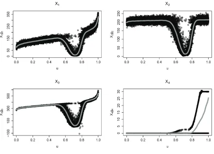
In Figure 1, the quantities xjigˆi(xj) are plotted as black circles, against uj = ˆFY(yj), such

that large values of u in the horizontal axis correspond to high outcomes of the outputY. The

grey line represents an estimate of the functionu7→si(u;X, g) =E Xigi(X)|UY =u

, obtained

again by local regression with a bandwidth of 0.01. As discussed in Section 2.2, averaging over

the curve si(u;X, g) with respect to weights ζ(u) yields Si(X, g).

It is seen that forX1, X2, X3, the plotted curves dip, representing a reduced sensitivity under

those scenarios where a payment from the reinsurer is received (the black circles that do not

follow that pattern correspond to observations xj4 = 1 where reinsurance default has taken

place). Thus, once the reinsurance layer is activated, small changes in those model inputs have

no effect on the value ofY. Once the layer is exhausted (i.e. for scenarios withyj > λ+l) the

sensitivity rises again.

Comparing the curves for X1 and X2, it is seen that (ignoring the dip in the curves) the

sensitivity toX2 is higher for low u, close to its higher mean of 200. However, the sensitivity to

X1 shows an increasing trend, ending up dominating for large confidence levels of the output, i.e.

foru >0.9. This reflects its higher volatility and the heavier tail of the LogNormal distribution

4_{Due to the small number of simulated scenarios in whichY is very high, it is possible that the local regression}

algorithm fails to produce reasonable gradients for some states. In this implementation, we did not use the 30

Figure 1: Sensitivity estimates in example 1. Each black circle represents an

observa-tion xjiˆgi xij; the grey line represents a non-parametric estimate of u 7→ si(u;X, g) =

E _{Xigi(X)|UY =u} .

used to model X1. The sensitivity to X3 also shows an increasing trend in u, even though the

volatility of X3 is low. This reflects the impact of the multiplicative effect of X3.

On the other hand, it is seen that the sensitivity curve s4(u;X, g) for X4 is zero up until

approximately u = 0.6. This corresponds to scenarios where the reinsurance layer is not

acti-vated, and thus reinsurance default is inconsequential. Then the black circles bifurcate. The

part that is stuck at zero corresponds to non-default events{X4 = 0}, while the increasing part

corresponds to default events {X4 = 1}. The curve increases up to l = 30 which is the

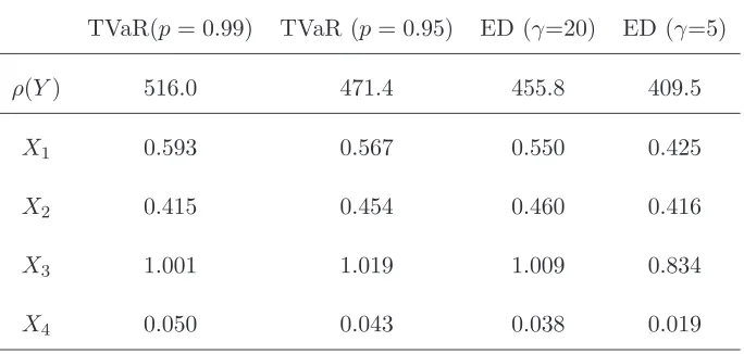
Table I: Scaled sensitivities Si(X, g)/ρ(Y) for a range of risk measures.

TVaR(p= 0.99) TVaR (p= 0.95) ED (γ=20) ED (γ=5)

ρ(Y) 516.0 471.4 455.8 409.5

X1 0.593 0.567 0.550 0.425

X2 0.415 0.454 0.460 0.416

X3 1.001 1.019 1.009 0.834

X4 0.050 0.043 0.038 0.019

the highest sensitivity is obtained, reflecting the fact that under those scenarios the maximum

recovery is due and will therefore be lost in the case of default.

In Table I, we report the sensitivities Si(X, g) to model inputs for two risk measures, TVaR

and Exponential Distortion (ED), at different levels of conservativism. The respective weight

functions are

ζT V aR(u;p) =

1

1−p1{u > p}, ζED(u;γ) =

γexp(γu)

exp(γ)−1. (3.5)

The TVaR risk measure places a constant positive weight to extreme loss scenarios (u > p)

and a weight of zero to all other scenarios. The ED risk measure places a positive weight to

all scenarios, strictly increasing inu, thus reflecting the whole of the output distribution. The

risk measures are ordered from left to right on the table, in terms of a decreasing weight placed

on the right tail of the output loss distribution, noting that ζT V aR(1; 0.99)> ζT V aR(1; 0.95) =

ζED(1; 20)> ζED(1; 5).

To enable comparison, the reported sensitivities are in each case scaled by the risk summary

ρ(Y), giving effectively a measure of elasticity to changes in model inputs. It is seen that the

highest sensitivity is to the multiplicative factorX3, followed by the LogNormal claimsX1. The

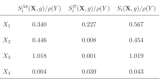
Table II: Breakdown of scaled sensitivities Si(X, g)/ρ(Y) to mean and deviation components,

for TVaR with p= 0.95.

S_iM(X, g)/ρ(Y) S_iD(X, g)/ρ(Y) Si(X, g)/ρ(Y)

X1 0.340 0.227 0.567

X2 0.446 0.008 0.454

X3 1.018 0.001 1.019

X4 0.004 0.039 0.043

used. The sensitivity toX4is not very high and reduces again as less tail-sensitive risk measures

are used. These observations are consistent with the previous discussion of Figure 1.

While the sensitivity values assigned to different inputs by the TVaR and ED measures are

different, the importance ranking produced is the same. In Example 2, it will be seen that

there are circumstances where the exclusive emphasis of TVaR on high outputs can make it

“blind” to sensitivities prevalent in less extreme scenarios. Note also that each point on the

curves u 7→ si(u;X, g) corresponds to sensitivity with respect to the VaRu measure, with the

importance ranking produced strongly dependent on the confidence levelu. Hence we would not

advise the use of a VaR measure at a single confidence level. More broadly, while a risk measure

such as ED can be used to produce a ranking between inputs, consideration of the full set of

curvesu7→si(u;X, g) in Figure 1 is helpful, as it allows the risk analyst to assess comparative

importance of inputs at different output confidence levels.

Further insight may be obtained by apportioning each sensitivity Si(X, g) to its mean and

deviation elements SM_i (X, g) and S_iD(X, g), as in (2.2). Such a decomposition for TVaR with

p = 0.95 is reported in Table II. It can be seen that the sensitivity to X1 is driven to a large

Similarly, the sensitivity to X3 is also driven by its mean due to the multiplicative effect of

inflation. On the other hand, the sensitivity to the indicatorX4 is mainly driven by variability.

In particular, focusing on the second column of the table, it is clear that the risk summaryρ(Y)

is more sensitive to the deviation element of the default indicator X4 than either X2 or X3.

4

EXTENSIONS

4.1 Sensitivity to model parameters

The model function g will generally be characterised by a number r of parameters, λ ₌

(λ1, . . . , λr), a dependence that has up to now been suppressed in the notation. If there is

uncertainty around these parameters, they can be treated as model inputs. Here we consider

the case where model parameters are known constants (such as λin Example 1). Thus we now

consider the model as a function of d+r arguments, such that Y = g(X,λ_{), where X is a}

random vector andλ _{is a vector of constants.}

A simple way of defining the sensitivity of ρ(Y) to the model parameter λk is to consider it

as a degenerate random variable with all probability mass concentrated at one point. Thus the

sensitivity to λk may be obtained as

Sd+k((X,λ), g) =λkE gd+k(X,λ)ζ(UY). (4.1)

Hence the sensitivity toλkis nothing butλkitself, multiplied by the corresponding model

func-tion gradient, averaged over scenarios of interest as specified byζ. Note thatS_dD_+k((X,λ_{), g) = 0.} The partial derivativegd+kis not directly obtainable via the local regression scheme of Section

3, since the simulated sample considered there will not supply any variability in the (d+k)th argument of g. A practical way of dealing with this issue is to randomize the parameter vector

λ_{, such that quantities g(X,Λ) are simulated, where Λ is a random vector of elements that}

randomization serves only numerical purposes and does not represent uncertainty in relation

to the value of λk. Once a local linear regression model has been estimated on that sample,

predictions of the model function and its gradients for fixedλ_{can be simply obtained from (3.2),}

by evaluating the non-parametric estimates at the points zj = (xj,λ). Although the choice of

the distribution for Λkis arbitrary, the measured sensitivity is robust to different choices. Indeed,

the volatility of Λk is only used to estimate the gradientgd+kand for sensitivity calculation the

conditioning Λk=λk applies.

4.2 Sensitivity to statistical parameter uncertainty

To study the sensitivity of the output to the uncertainty of statistical parameters, we specify

the distribution of each model input conditionally on the parameters. In particular, we assume

that Xi|Θi =θi∼F(·|θi). The distribution Gi of the random variable or vector Θi reflects the

uncertainty pertaining to the value of the parameters of the distribution ofXi.5

For evaluation of the risk summary and of sensitivities, the unconditional distribution ofXi,

given by ˆFi(x) =

R

Fi(x|θ)dGi(θ) is used. In particular, when a Monte-Carlo sample is produced,

in every state a different observation from Θi is obtained, and subsequently an observation of

Xigiven that outcome of Θiis simulated. Thus Θiis allowed to vary across simulated scenarios.

As opposed to the case of model parameters discussed in Section 4.1, we do not attempt to

“smooth out” the uncertainty in Θi, but retain it as an explicit feature of the model.

Our purpose now is to calculate the sensitivity of ρ(Y) to each of Θ1, . . . ,Θd. To do this,

we express each model input Xi as a function of Θi, representing parameter uncertainty, and

another random variable Zi, representing pure process (stochastic) uncertainty. This can be

achieved, for a conditional distribution Fi, by setting Ui = Fi(Xi|Θi) and Zi = Fi−1(Ui|θˆi),

5_{Taking a rather pragmatic view, we do not specify the provenance ofG}

i – it may be derived by a bootstrap

where ˆθi = E(Θi) is an unbiased estimate of the unknown parameter. Then we have that Zi

follows the distributionFi with parameter ˆθi and is independent of Θi. The precise statement

of this argument is given in Appendix C, Lemma 9.

As a result, we can expressXi asXi =ψ(i)(Zi,Θi),where the first and second arguments of

ψ(i) represent the contribution of process and parameter uncertainty to Xi respectively.

There-fore, following Lemma 6 in Appendix B, the sensitivities to Zi and Θi can be respectively

calculated as

E _Zigi(X)ψ(i)

1 (Zi,Θi)ζ(UY)

E _(Θi−θˆ_i)gi(X)ψ(i)

2 (Zi,Θi)ζ(UY)

. (4.2)

For parameter uncertainty we propose the use of the deviation component of sensitivity only.

This is because a marginal change in Θi may be hard to interpret in the context of parameter

uncertainty; on the other hand it is plausible to reduce the volatility of Θi via diligent data

collection, expert judgement and further analysis. While it may be possible to evaluate (and

differentiate) the functionsψ(i)analytically, when working with a Monte-Carlo sample, they can be estimated directly from the data by local linear regression.

The following example builds on Example 1. By considering the sensitivity to known model

parameters, we are able to quantify the importance of the “constants” found in any model, such

as the initial inventories of radionuclides in the Level E model(7)_{. The importance of those}

constants is assessed in the context of a global sensitivity analysis, since it still depends on

the variation of the uncertain inputs. Furthermore, we consider the uncertainty in statistical

parameters; this, though simpler, parallels the stochastic volatility model described by Saltelli

et al. (Sec. 6.2, Ref.(5)), where the variance of a diffusion process is endowed with its own

dynamics.

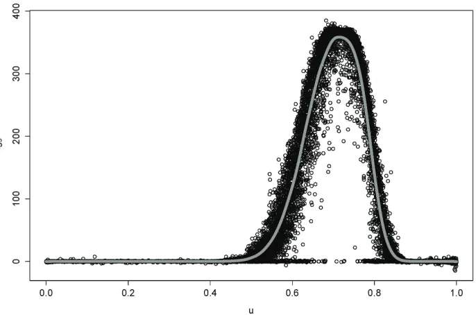
Figure 2: Sensitivity to λ in example 2. Each black circle represents an observationλgˆ5 xij

;

the grey line represents a non-parametric estimate of u7→s5(u;X, g) =λE g5(X)|UY =u .

deductible parameterλ. For this purpose we run the simulation with a randomized deductible,

uniformly distributed around the known value of λ= 380, such that Λ ∼U nif[375,385]. The

corresponding plot of the estimated sensitivity function s5(u; (X, λ), g) is given in Figure 2 and

the scaled sensitivitiesS5(u; (X, λ), g) for different risk measures are collected in the first row of

Table III.

From Figure 2 it is seen that the sensitivity to λ is positive for that range of confidence

levels of output where the reinsurance layer is used but not exhausted. Since the parameter lis

unchanged, the positive sensitivity represents the fact that for a higher deductible, reinsurance

recoveries will be less frequent. The sensitivity is zero for low confidence levels, as in those

scenarios the reinsurance layer is not used. It is also zero for high confidence levels, corresponding

to situations where the layer is exhausted and the exact loss level at which the layer was activated

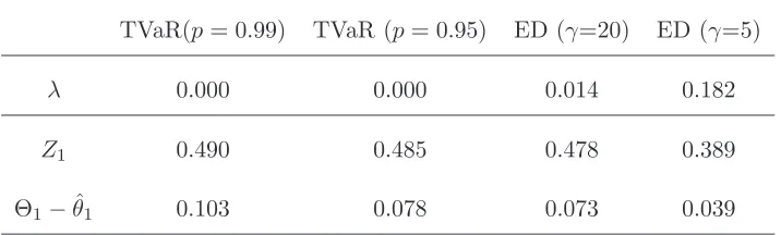
Table III: Scaled sensitivities to λ, Z1,Θ1 for a range of risk measures.

TVaR(p= 0.99) TVaR (p= 0.95) ED (γ=20) ED (γ=5)

λ 0.000 0.000 0.014 0.182

Z1 0.490 0.485 0.478 0.389

Θ1−θˆ1 0.103 0.078 0.073 0.039

sensitivities to the TVaR measures is zero, since these risk measures only consider scenarios at

the far tail of FY, where the reinsurance layer is completely used up. This shows that a risk

measure such as ED, assigning a positive weight at all confidence levels, may be preferable to

TVaR. The example also demonstrates the usefulness of plotting the sensitivity function at all

confidence levels, in order to detect local effects.

Now we consider the case of parameter uncertainty in the claims from the first line of business.

We assume that there is some uncertainty around the first parameter of the distribution ofX1.

In particular we let X1|Θ1 ∼ LogN ormal Θ1, σ21

and Θ1 ∼ N ormal(ˆθ1, σ2Θ1). After simple

manipulations involving Normal and LogNormal distributions, the decomposition ofXi becomes

X1 =ψ(1)(Θ1, Z1) = exp(Θ1−θˆ1)Z1,

whereZ1∼LogN ormal θˆ1, σ21

. The specific parameters chosen are ˆθ1= 4.99, σ1 = 0.230, σΘ1 =

0.163, such that the unconditional moments of X1 are (consistently with Example 1) E(X1) =

153, V_{(X1) = 44}2_{, while conditional moments are}E_{(X1|Θ1 = ˆθ1) =}E_{(Z1) = 151,} V_{(X1|Θ1 =}

ˆ

θ1) =V(Z1) = 352.

The sensitivities toZ1 and Θ1−θˆ1, calculated according to (4.2), are reported in the second

and third row of Table III. It is seen that, particularly for the tail-focused TVaR measures, the

4.3 Sensitivity to the dependence structure

Finally, we turn our attention to studying the sensitivity of the output risk summary to the

dependence structure. We propose an approach that is applicable for dependence structures that

display conditional independence, given some observable or latent common model inputs; the

latter appear implicitly in standard dependence models, such as the popular class of Archimedean

copulas (see Ref.(32), Sections 3.4.1 and 5.4). The idea pursued here is to express each model

input Xi as

Xi=ψ(i)(Zi,V), (4.3)

where the random variables Z1, . . . , Zd are independent and V is the vector of common model

inputs.

Henceforth, we call the elements of V thecommon factors and Z1, . . . , Zdthe idiosyncratic

factors. When the common factors are explicitly modelled and have a direct interpretation

(e.g. as natural catastrophe losses, affecting different parts of an insurance portfolio), the

representation (4.3) is essentially given. In the case that common factors are implicit in the

dependence structure, then the representation (4.3) is again possible by the following

argu-ment. For presentational simplicity, let us assume that Fi(·|v), the conditional distribution of

Xi given V = v, is invertible. Then, to obtain the idiosyncratic factor Zi, we may just set

Zi =Hi−1(Fi(Xi|V)), whereH is an arbitrary distribution (a plausible choice may be to let Hi

be the unconditional distribution of Xi). Then,Zi will be independent of V and we can write

Xi = ψ(i)(Zi,V) = F_i−1(Hi(Zi)|V). A precise statement of these facts is given in Lemma 10,

Appendix C.6

6_{By its construction,ψ}(i) _{is increasing in its first argument. A particular case of interest emerges ifV ≡V}

is 1-dimensional and ψ(i) _{is also increasing in the second argument for all i. In that case, X}

i is stochastically increasing inV and the random vectorX_isassociated; see Property 7.2.16 in Ref.(30). Thus, each element of the

The sensitivity to the dependence structure may now be studied by calculating the sensitivity

to the common and idiosyncratic factors. For simplicity consider a univariate common factor

V. Then the sensitivity of output risk summary to Zi and V can be respectively calculated as

E _(Zi−E_(Zi))gi(X)ψ(i)

1 (Zi, V)ζ(UY) (4.4)

d

X

j=1

E _{(V −}E_(V))gj(X)ψ(j)

2 (Zj, V)ζ(UY). (4.5)

We emphasize the deviation component of the sensitivities, since the prime effect of the

depen-dence ofX is on the variability of the output.

The proposed process is demonstrated via the following example, where sensitivity to the

dependence between the output loss of Example 1 and an investment position is studied. The

importance of dependence between inputs is recognised widely in sensitivity analysis, e.g.(5,7),

but, to our knowledge, the sensitivity to factors driving such dependence has not been studied

in the literature.

Example 3. To allow the focus on dependence, here we consider a simple extension to Example

1. Assume that assets are invested that produce income A, with expected value equal to that

of the total lossY. The random variableA is not independent ofY. After taking into account

such investment, the loss becomes ˜Y =Y −A. For consistency with the notation of this section,

we re-label the variables as ˜X1 ≡Y, X˜2 ≡ −A, such that

˜

Y = ˜g( ˜X1,X˜2) = ˜X1+ ˜X2.

Therefore ˜Y is now the model output, arising through simple addition of the inputs ˜X1,X˜2.

The random variable ˜X1 ≡Y has the same distribution as in Example 1, denoted here by

H1. The asset valueA=−X˜2 follows a LogN ormal(5.894,0.12) distribution. The distribution

of ˜X2 is denoted by H2. For those parameters it is E( ˜X1 + ˜X2) = 0, such that assets match

liabilities on average.

The dependence between ˜X1 and ˜X2 is modelled via a Clayton survival copula, with Kendall

rank correlation coefficient ofτ = 0.5. This is the copula of a bivariate Pareto distribution with

parameter α = 0.5(1/τ −1) = 0.5 (Section 5.4 in Ref.(32)_{). For this model, we can express}

˜

X1,X˜2 as non-decreasing functions of the bivariate Pareto random variables X1′, X2′, defined

by X₁′ =D1V′, X2′ = D2V′, where D1 and D2 follow exponential distributions with mean 1,

1/V′ _{is Gamma distributed with shape parameter equal to α = 0.5 and scale parameter 1,}

and the random variables D1, D2, V′ are independent (Section 7.2.4 in Ref.(30)). It is evident

that (X₁′, X₂′), and therefore ( ˜X1,X˜2) are independent conditional onV′. Because of the simple

multiplicative structure, there is no need to invoke the construction of Lemma 10.

Consistently with previous arguments, we let the random variables Z1 ∼H1, Z2 ∼H2 and

V ∼ U nif[0,1] be non-decreasing functions of D1, D2, V′ respectively. Thus the independent

random vector (Z1, Z2) has the same marginal distributions as ( ˜X1,X˜2). A uniform distribution

is chosen for the common factorV, since the latent variableV′ lacks a natural interpretation in

the present application.

For a simulated sample of 20000 observations, the sensitivities toZ1, Z2andV are calculated.

The gradients of the functions ψ(1), ψ(2) are once more calculated numerically by local linear

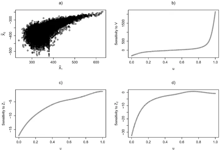
regression (we treat the gradient of ˜gas given). A pictorial summary of the resulting analysis is

provided in Figure 3. In panel a) a scatter plot between ˜X1 and ˜X2 is given showing the very

strong dependence for high output values, representing joint adverse events. In panels b), c)

and d), estimates of the functions

u7→E _{V −}E_(V)

ψ₂(1)(Z1, V) +ψ(2)2 (Z2, V)|U_Y˜ =u

;

u7→E _Z1−E_(Z1)

ψ(1)₁ (Z1, V)|U_Y˜ =u

;

u7→E _Z2−E_(Z2)

ψ(2)₁ (Z2, V)|U_Y˜ =u

;

Figure 3: Analysis of the sensitivity to the dependence structure. a) Scatter plot of ˜X1,X˜2;

b) Sensitivity to common model input V; c) Sensitivity to idiosyncratic model input Z1; d)

Sensitivity to idiosyncratic model inputZ2.

dominates those of the idiosyncratic factorsZ1 andZ2for high confidence levelsu. In particular,

at those levels the sensitivities toZ1, Z2 are approaching zero, supporting the intuitive view that

scenarios of extreme output are “driven by dependence”.

5

CONCLUSIONS

A framework for global sensitivity measurement using directional derivatives of risk measures

has been developed. We focused on the class of distortion risk measures, while our arguments

also work for moment-based risk measures, which may be preferred in some applications.

The proposed sensitivity analysis method is applicable to Monte-Carlo samples of non-linear

estimation, if an analytical expression for the gradient is unavailable or hard to work with. It

was shown through examples drawn from insurance loss modelling that informative percentile

sensitivity curves can be produced as outputs of the sensitivity analysis exercise, aiding a risk

analyst in understanding the ways in which inputs and output interact. In this both the modelled

statistical behaviour of model inputs and the non-linearity of the model function are reflected.

Finally, it was demonstrated how the sensitivity measure can be extended to cope with

structural parameters, uncertain statistical parameters and common factors driving dependence.

APPENDIX: FORMAL STATEMENTS AND PROOFS

A

PROOF OF PROPOSITION 2

The technical conditions required for Proposition 2 include differentiability of g (condition i)),

which will not always hold. However, in applications model functiongwill need to be estimated.

In such a context, for reasons of tractability a smooth model is typically used to approximateg

– this process was demonstrated in Section 3. Moreover, when the model function is continuous

and non-differentiable at only a countable number of points, the proof of Proposition 2 still

holds. Condition ii) is relatively weaker; for example any model function that can be written

asg(X) =g(1)(Xk) +g(2)(X−k), where g(1) is an invertible function andXk|X−k is continuous,

will satisfy this. Condition iii) is implied from i) and ii) plus some integrability conditions that

we do not explicitly state, as they are similar to those in(24).

First, in Lemma 3 the derivative of the percentile function with respect to a proportional

shock on Xi is worked out. The proof is a direct generalization of an argument given by

Tasche(24)in the case of linear models. A related result, under somewhat different assumptions,

is obtained by Hong(25).

a conditional density given (X2, . . . , Xd), denoted φ(·|x2, . . . , xd). Let the function g :X → R

be differentiable in the ith argument with ∂g_∂x(x)

i =gi(x) and invertible with respect to x1 for all

x2, . . . , xd. Define Y = g(x1, . . . , xd) and Yi,t = g(X1, . . . , tXi, . . . , Xd) and the corresponding

quantile function ηi,u(t) =FY−1i,t(u). If ηi,u(t) is differentiable at t= 1 for given u∈(0,1), then

η′_i,u(1) =E_{(Xigi(X)|g(X) =ηi,u(1)).}

Proof. Drop the subscript inηi,u, denote byl the inverse ofg(assumed increasing) with respect

to the first argument and let X−1= (X2, X3, . . . , Xd).

Let us show first that the density of Y is

y→fY(y) =E(φ(l(y,X−1)|X−1)l1(y,X−1)) =

=E

φ(l(y,X−1)|X−1)

g1(l(y,X−1),X−1)

.

For a given nonnegative function k, we have

E_{(k(Y)|X−1) =}E_{(k(g(X1,X−1))|X−1)}

= Z +∞

−∞

k(g(x1,X−1))φ(x1,X−1)dx1

= Z +∞

−∞

k(y)φ(l(y,X−1)|X−1)

1

g1(l(y,X−1),X−1)

dx1,

after making the change of variable g(x1,X−1) = y and observing that dx1 = dl(y,X−1) =

1

g1(l(y,X_−1),X₋₁₎. It follows that the conditional density of Y given X−1 is

y→φ(l(y,X−1)|X−1)

1

g1(l(y,X−1),X−1

.

From this we immediately deduce the unconditional density of Y.

Consider the case i= 1. Using the definition of quantile we have

so that, usingl and conditioning onX−1, this becomes

u=E

P

X1 ≤

1

tl(η(t),X−1)|X−1

=

=E

Z l(η(t),X−1)/t −∞

φ(x1|X−1)dx1 !

.

Taking derivatives with respect to t, exchanging the derivative with the expectation and

letting thent= 1, gives

0 =E _{φ(l(η(1),X−1)|X−1)}

l1(η(1),X−1)η′(1)−l(η(1),X−1) .

Solving with respect toη′(1) we get

η′(1) = E(l(η(1),X−1)φ(l(η(1),X−1)|X−1)) E_{(l1(η(1),X−1)φ(l(η(1),X−1)|X−1))}.

Now, let us compute the conditional expectation E_{(X1g1(X)|Y). For any nonnegative function}

k, we have

E_{(X1g1(X)k(Y)) =}E₍E_{(X1g1(X1,X−1)k(Y))|X−1)}

=E

Z +∞

−∞

x1g1(x1,X−1)k(g(x1,X−1))φ(x1|X−1)dx1

=E

Z +∞

−∞

l(y,X−1)k(y)φ(l(y,X−1)|X−1)dx1

= Z +∞

−∞

k(y)E(l(y,X−1)φ(l(y,X−1)|X−1))

fY(y)

fY(y)dy

=E_(k(Y)q(Y)),

with

q(y) = E(l(y,X−1)φ(l(y,X−1)|X−1))

fY(y)

= E(l(y,X−1)φ(l(y,X−1)|X−1)) E_{(l1(y,X−1)φ(l(y,X−1)|X−1))}

so we conclude that

E_{(X1g1(X1,X−1)|Y) =q(Y),}