Development of a two-temperature open source CFD model for hypersonic reacting flows

Development of a Two-Temperature Open-Source

CFD Model for Hypersonic Reacting Flows

Vincent Casseau

, Thomas J. Scanlon

and Richard E. Brown

The highly complex flow physics that characterise re-entry conditions have to be repro-duced by means of numerical simulations with both an acceptable level of accuracy and within reasonable timescales. In this respect, a new CFD solver, hyFoam, has been devel-oped within the framework of the open-source CFD platform OpenFOAM for modelling hypersonic reacting flows. hyFoam has been successfully validated for two 0-degree adia-batic heat bath test cases and the limitations of a one-temperature CFD model have been highlighted. To cope with high-temperature gas chemistry, the internal energy has been decomposed into its elementary energy modes, thus introducing the translational-rotational and the vibrational temperatures. A two-temperature CFD model is being implemented in order to attain a better agreement between CFD and DSMC results. Validation of the code for a single species has been executed while mixture-related libraries are currently being developed. The vibrational-translational relaxation time formulation has also been presented and discussed.

Nomenclature

Symbols

β temperature exponent in the Arrhenius law δ Kronecker delta

ζ degree of freedom

θv characteristic vibrational temperature κ thermal conductivity

λ bulk viscosity Λ series of coefficients µ shear viscosity ρ gas density

ρk partial density of species k σv limited collision cross-section

τ shear stress tensor

τ_V−T vibrational-translational relaxation time

˙

ω net mass production of species

A pre-exponential factor in the Arrhenius law ¯

c average molecular speed C species concentration

e energy per unit mass of species E total energy

Et,r,v energy associated with one energy mode Fi flux vectors

h enthalpy per unit mass of species h◦ chemical enthalpy

J species diffusion vector kf forward reaction rate constant

Mi molecular weight of speciesi

Mjk reduced mass of speciesj andk n number density

p pressure

q heat conduction vector

Q_V−ch vibration-chemistry coupling source term

Q_V−T vibrational-translational energy transfer Q_V−V vibrational-vibrational energy transfer R specific gas constant

s number of species in the mixture T temperature or overall temperature Ta temperature of activation

Tt,r,v molecular temperatures

u,v,w components of the velocity vector U vector of conserved quatities

v diffusion velocity vector

˙

W source vector

X species molar fraction Zr rotational collision number

∗_{PhD Researcher, Department of Mechanical and Aerospace Engineering, Student Member AIAA.} †_{Senior Lecturer, Department of Mechanical and Aerospace Engineering.}

‡_{Professor and Director of the Centre for Future Air-Space Transportation Technology (cFASTT), Department of Mechanical}

Subscripts and superscripts int internal

r rotational t translational

tr translational-rotational v vibrational

0 initial

I.

Introduction

H

vision of air-space transportation. From an engineering, environmental and societal viewpoint, consid-erable obstacles remain to be resolved to make this future a reality.1 _{One of the barriers that needs to be}

overcome concerns the thorough understanding and characterisation of the aerothermodynamic flow condi-tions experienced by the vehicle as it enters the Earth’s atmosphere.2 _{This point is of crucial importance to}

preserve the integrity of the aircraft in the searing conditions of the descent phase.

The highly complex flow physics that characterise re-entry conditions have to be reproduced by means of numerical simulations with both a good level of accuracy and within reasonable timescales. Hypersonic re-entry vehicle flow fields at intermediate altitudes - ranging from 60 to 80 km - contain a mixture of continuum and non-continuum (rarefied) regions. Navier-Stokes solutions using conventional computational fluid dynamics (CFD) are appropriate for continuum flows but fail to accurately predict non-continuum flow behaviour. Conversely, the direct simulation Monte Carlo (DSMC) particle-based methodology is the preeminent technique for rarefied flows but requires significant computational effort when solving continuum regions. The craft may also encounter a chemically reacting environment that can have a significant influence on aerodynamic performance and surface heating. Numerical models that fail to incorporate such reacting flows miss an essential part of the flow physics surrounding the vehicle.

The need for reliable numerical tools that can capture thermochemical non-equilibrium with high-fidelity has gained momentum recently, principally due to NASA’s upcoming critical missions involving the next Crew Exploration Vehicle, Orion,3 _{and complex systems to allow high-mass payload entries in the}

Mar-tian atmosphere.2 _{Among the most popular CFD codes dedicated to the study of the hypersonic regime}

are NASA’s DPLR4 _{(Data-Parallel Line Relaxation) and LAURA}5 _{(Langley Aerothermodynamic Upwind}

Relaxation Algorithm), VULCAN6_{(Viscous Upwind aLgorithm for Complex flow ANalysis), US3D}7,8

(Un-Structured 3D) of the University of Minnesota, and LeMans9,10 _{(the Michigan Aerothermal Navier-Stokes}

Solver) of the University of Michigan. They have all adopted a similar strategy to cope with thermochemical non-equilibrium where the gas mixture is no longer described by a single temperature but by at least two distinctmolecular temperatures.11 These temperatures are derived from the decomposition of the internal energy into its elementary energy modes thus distinguishing the translational-rotational temperature from its vibrational counterpart. Each of the CFD codes described above contain differences which are mainly due to the distinct representation of energy exchange between the energy modes.3

In order to address the issues described above a new CFD solver has been developed within the framework of the open-source CFD platform OpenFOAM12 _{for modelling hypersonic reacting flows. Contributions of}

competing mechanisms are considered in isolation by focusing on a 0-degree adiabatic heat bath and by validating the chemistry module independently from the two-temperature model. Lack of experimental or flight data and uncertainties in the determination of reaction rates and relaxation times force us to reflect upon any comparisons between the CFD and DSMC results, DSMC being often regarded as an experimental analogue. Hence, the DSMC solver,dsmcFoam, developed and validated13,14_{at the University of Strathclyde,}

II.

Methodology

The work that has been carried out within OpenFOAM can be split into two main sections. The first consisted of improving and validating the current chemistry module using a standard one-temperature model. This then set the basis for a two-temperature CFD arrangement. These are the two stages that are presented in the following sub-sections. Ultimately, the chemistry part and the new thermodynamic libraries will be reunited to form a two-temperature solver for simulating high-temperature reacting mixtures.

A. Chemistry solver

A suitable OpenFOAM CFD solver, rhoCentralFoam, has first been identified and assessed. This solver has been created to resolve high-speed compressible flows,17 _{making use of central-upwind interpolation}

schemes of Kurganov and Tadmor.18 _{It has produced comparable results to those given by the MISTRAL}

flow solver,19 _{for continuum hypersonic simulations over a hollow cylinder.}20 _{Basic chemistry features have}

been added to rhoCentralFoam by incorporating parts of the solver reactingFoam, an OpenFOAM solver dealing with combustion. This enables us to include chemical reactions along with their type and rates and to introduce quantities related to the species mixture, such as mass fraction or number density. The newly blended code has been given the name hyFoam. The solution process then consists of resolving a set of ordinary differential equations (ODE) and species mass fractions. Validation of the new code implementation has been carried out by initially considering the reversible reaction of hydrogen and iodine to produce hydrogen-iodide in the reaction I₂+ H₂ −−₎₋₋* 2HI. This chemical reaction occurs at constant temperature and an analytical solution of the species concentration over time can be easily derived.21 The forward and reverse rate constants at T = 700 K are also to be found in the aforementioned reference. Species concentrations plotted with respect to time for both the analytical solution andhyFoam are shown in Figure1. The results demonstrate a highly satisfactory agreement thus validating this first stage of the newhyFoam solver implementation.

0 1 2 3 4 5 6 7 8

0 5 10 15 20 25

Species concentration,

CHI

,

[mol / m

3 ]

Time, t [h]

I₂ + H₂ ↔ 2HI

C0_I

2 = C 0

H2 = 4.54 mol / m

3

analytical

hyFoam CI

2

,

CH

2

Figure 1. Species concentration versus time for a chemically reacting H₂- I₂reservoir at a constant temperature

of 700 K and an initial pressure of 0.528 atm.

B. Governing equations

1. Two-temperature model

Decomposition of the internal energy into its elementary energy modes is a consequence of the Born-Oppenheimer approximation.23 Although its validity has been debated by Giordano,24 this approach un-doubtly remains the reference as it has proved to give satisfactory results for numerous re-entry case sce-narios.25,26,27 Moreover, as Bird has indicated, when it comes to the numerical modelling of a physical phenomenon, a gain in physical realism does not necessarily translates into improved results.15

The study of the ionised flow-field is outside of the scope of this paper and as such the electron-electronic energy mode is disregarded in the following. The total energy, E, can be decomposed as the sum of the kinetic, translational, internal, and chemical energies as follows28

E = 1

2ρuiui + s X

k=1

Et,k + s X

k=1

Er,k + s X

k=1

Ev,k + s X

k=1

ρkh ◦

k (1)

where indicest, r, andv refer to translational, rotational, and vibrational energy modes, respectively. k is an index to vary between 1 and the number of species in the mixture,s. ρis the mixture density andui for ito vary between 1 and 3 denotes one of three components of the velocity vector. ρk stands for the partial density of species k and h◦_k is the standard enthalpy of formation of species k. In particular, the relation between the vibrational energy,Ev, and the vibrational energy per unit mass of speciesk,ev,k, is given by

Ev= s X

k=1

Ev,k= s X

k=1

ρkev,k (2)

The translational and rotational energy modes are fully excited below a few tens of Kelvin and the relaxation towards equilibrium of the translational and rotational temperatures, denoted by Tt and Tr, respectively, is known to be achieved within a small number of particle collision events.15 Hence, Tt and Tr are considered to be identical, called the translational-rotational temperature, and designated by Ttr. Depending on the type of particle under investigation, the internal energies per unit mass of species may be written as atoma         

et,a = 3/2×RaTtr er,a = 0

ev,a = 0

(3) molecule m

        

et,m = 3/2×RmTtr er,m = RmTtr

ev,m =

Rmθv,m

expθv,m Tv,m

−1

(4)

whereRis the specific gas constant, equal to the ratio of the universal gas constant divided by the molecular weight of the particle, and θv is the characteristic vibrational temperature of the particle of interest. A simple harmonic oscillator is employed for the vibrational mode.15

Coupling between the translational-rotational and vibrational energy modes, denoted by Qk,V−T, is

then quantified using the Landau-Teller equation.29 _{This equation prescribes the}

translational/rotational-vibrational (V-T) energy exchange rate and thus the time rate of change in translational/rotational-vibrational energy as follows

Qk,V−T =ρk

∂ev,k(Tv,k) ∂t =ρk

ev,k(Ttr)−ev,k(Tv,k) τk,V−T

(5)

whereτk,V−T is the molar averaged V-T relaxation time.

Millikan and White30 _{proposed a semi-empirical correlation to estimate the V-T relaxation time for a}

large variety of species. The formula is valid for temperatures within the range [300; 8,000] K. In the worst case scenario divergence from the experimental measurements is observed up to a factor of 5. For a mixture, this yields

τk,V−T =τ M W k =   s X j=1

Xj/τjk,V−T 



−1

whereX is the species molar fraction and the interspecies relaxation times,τjk,V−T, can be written as

τjk,V−T =

1 pexp

h

Ajk

T_tr−1/3−0.015M_jk1/4−18.42i withpin atm (7) CoefficientAjk and the reduced mass of speciesj andk,Mjk, are given by

Ajk= 1.16×10−3 p

Mjkθ 4/3

v,k (8)

Mjk=

MjMk

Mj+Mk

(9)

whereMk is the molecular weight of speciesk in g/mol.

Park added a correction factor to the Millikan-White formula31 _{to take into account the inaccurate}

estimation of the collision cross-section at high temperatures. The V-T relaxation time is now defined by

τk,V−T =τ M W

k +τ

P

k (10)

where the collision-limited relaxation time,τP

k, is a function of the average molecular speed, ¯ck, the limited collision cross-section,σv, and the number density as follows

τ_kP = 1 ¯ ckσvnk

(11)

with

¯ ck=

r

8RkTtr

π (12)

and σv= 10−21

_50,000

Ttr 2

(13)

Vibrational-vibrational coupling, QV−V, and chemistry-vibration coupling,QV−ch, are beyond the scope

of this paper and will be implemented and investigated in future studies.

Finally, the overall temperature, T, is reconstructed considering a formula involving molecular tempera-tures and their respective degrees of freedom. This may be written as

T =3Tt+ ¯ζintTint 3 + ¯ζint

(14)

An analogous expression can be found in Bird’s book15 _{to determine the overall temperature from any}

DSMC computations. The subscript intrefers to the internal energy modes which are in the present case the rotational and vibrational modes. ζ is the number of degrees of freedom in relation to one specific energy mode. Both translational and rotational energy modes are supposed to be fully excited, therefore, three degrees of freedom are allocated to the translational mode and ζt = 3. Neglecting the degree of freedom of rotation along the nuclear axis for diatomic molecules, two degrees of freedom are associated with the rotational energy mode if the particle is a molecule. Different values taken by ζ can be derived from equipartition theory, with

er= 1

2ζrR Ttr (15) and ev =

1

2ζvR Tv (16)

where ¯ζint is the mass-weighted average ofζr andζv.

2. Non-equilibrium Navier-Stokes-Fourier equations

The Navier-Stokes-Fourier (NSF) equations are solved to compute transient compressible reacting flows. These are presented below in flux-divergence form for the s species transport and reaction equations, the momentum equations, the vibrational energy equation, and the total energy equation. It states

∂U ∂t +

∂Fi ∂xi

=W˙ (17)

where the vector of conserved quantities,U, writes

U= (ρ1, ρ2, · · ·, ρs, ρu, ρv, ρw, Ev, E) T

u,v, and ware the three components of the velocity vector. The flux vectors,Fi, are given by

Fi =                       

ρ1ui+J1, i ρ2ui+J2, i

.. . ρsui+Js, i ρuiu+δi1p+τi1

ρuiv+δi2p+τi2

ρuiw+δi3p+τi3

Evui+qv,i+ s X

k=1

Ev,kvk,i

(E+p)ui+ 3 X

j=1

τijuj+qtr,i+qv,i+ s X

k=1

hkJk,i                        (19)

where indexirefers to one of the three dimensions of space andδ is the Kronecker delta. hk stands for the enthalpy per unit mass of speciesk. τ is the shear stress tensor and Stokes’ hypothesis for the bulk viscosity is assumed to hold. Thus

τij =−µ _∂u

i ∂xj

+∂uj ∂xi

−λ∂uk ∂xk

δij with λ=− 2

3µ (20)

whereµis the shear viscosity and λis the bulk viscosity.

Components of the heat conduction vector,q, are assumed to follow Fourier’s heat law

qtr,i=−κtr ∂Ttr

∂xi

qv,i=−κv ∂Tv ∂xi

(21)

where the thermal conductivityκis decomposed into translational-rotational and vibrational contributions. Please refer to Ref. 28for further detail.

Jk, i are the components of the species diffusion vector for species k defined as the product of the partial densityρk and the corresponding component of the diffusion velocity vector,vk,i. Their implementation in the OpenFOAM framework is planned in due course. Therefore, it can be considered in the following that diffusion velocities are equal to zero.

The source term vector,W˙, is given below

˙

W = ω˙1, ω˙2, · · · , ω˙s, 0, 0, 0, s X

k=1

Qk,V−T +Qk,V−V +Qk,V−ch

, 0

!T

(22)

where ˙ωk is the net mass production of speciesk.

III.

Results

A. One-temperature chemistry solver validation at high temperatures

A 0-degree adiabatic heat bath considering relaxation towards thermochemical equilibrium provides a good benchmark case to check how well the newhyFoam CFD code performs in relation to high-temperature gas chemistry. The test case is composed of a single cubic cell of length 1×10−5_{m and initial pressure of 0.063}

atm. Five different initial temperatures have been considered to cover a range of temperatures during the molecular dissociation, these beingT0_{={5, 7.5, 10, 15, 20} ×10}3_{K. The time-step for CFD computations}

has been set at 2×10−9_s.

The chemical reaction considered is the irreversible molecule-molecule dissociation of oxygen

O₂+ O₂−k−−−f(T→) 2O + O₂

The forward rate constant,kf, is assumed to follow the Arrhenius law, and is thus expressed by

kf(T) =A×Tβexp

−Ta

T

whereAis a pre-exponential factor,β is the temperature exponent, andTa is the temperature of activation derived from the activation energy. The units ofA andTa are given inm3/mol/sand Kelvin, respectively. Three sets of forward rate constants are employed : rates from Quantum Kinetic (QK) theory,13_{rates from}

the Dunn and Kang (DK) experiments,32,33_{and Park’s rates for the use of a two-temperature model (P2T).}31

A single temperature has been employed to represent all of the internal modes and the rate coefficients are shown in Table1.

Table 1. Parameters for the evalution ofkf

Reaction rate Arrhenius law constants

A β Ta

QK 3.21×1019 _{-1.0 59,370.6}

DK 3.24×1019 -1.0 59,883.0 P2T 2.0×1021 -1.5 59,500.0

In the DSMC calculations, an ensemble average of three statistically-independent solutions has been carried out. The time-step for DSMC computations has been set at 1.52×10−9 _{s as prescribed in Ref. 13.}

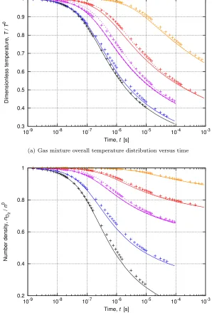
The comparisons betweenhyFoamanddsmcFoam are shown in figures2(a)and2(b). Results using DK rates are not displayed for reasons of clarity. P1T refers to P2T reaction rates when using a single-temperature model. Firstly, considering the QK rates for an initial temperature of 10,000 K, the hyFoam predictions are seen to be in excellent agreement with those provided by Boyd’s analytical code.13 hyFoam has thus been validated for a single, irreversible chemical reaction of dissociation involving O₂. However, it is evident that none of the reaction rates presented in Table 1 demonstrate a satisfactory agreement between CFD and DSMC results. For each initial temperature considered, the rate of change in temperature and species concentration is overpredicted using the CFD one-temperature model. This benchmark case illustrates the limitations of a one-temperature model for the study of dissociating mixtures. According to Bird,15 _”the

quantum treatment of vibration permits a physically realistic treatment of dissociation (p.52).” Therefore, it is essential to quantify the vibrational energy mode, i.e., split the internal energy into its separate energy modes, and to model the energy exchange between these modes. It is this two-temperature formulation that is discussed for single-species gases in the two subsequent paragraphs.

B. Vibrational-Translational relaxation of a single-species gas

The single-temperature OpenFOAM CFD solverhyFoam serves as the foundation of the newly coded solver hy2Foamthat incorporates the two-temperature model. The 0-degree adiabatic heat bath will again provide a first benchmark case for the validation of the implementation of the two-temperature model. Emphasis is made on vibrational-translational (V-T) relaxation. For this purpose, the same single cubic cell filled with O₂ is now set-up with different initial translational and vibrational temperatures. The translational temperature is set to 20,000 K while the vibrational temperature is lowered to 300 K. To further simplify the problem and solely investigate V-T energy transfers, chemical reactions of dissociation are disabled. Thus, the gas is composed of a single species.

dsmcFoam intrinsically has three temperatures : translational, rotational, and vibrational. However, in the event of a rotational collision number, Zr, set to unity, the rotational energy mode will always be in a state of thermal equilibrium and Tr will equal Tt to form Ttr. Tuning the value of Zr allows us to draw a direct comparison between the dsmcFoam and hy2Foam CFD results. Other CFD and DSMC settings remain unchanged.

Due to the inherent uncertainties arising from the experimental determination of the vibrational-trans-lational relaxation time, τ_V−T, it is considered unlikely that the Millikan-White correlations with (MWP)

0.3 0.4 0.5 0.6 0.7 0.8 0.9 1

10-9 10-8 10-7 10-6 10-5 10-4 10-3

Dimensionless temperature,

T

/

T

0

Time, t _[s]

(a) Gas mixture overall temperature distribution versus time

0.2 0.4 0.6 0.8 1

10-9 10-8 10-7 10-6 10-5 10-4 10-3

Number density,

nO

2

/

n

0

Time, t _[s]

(b) O₂ molecule concentration versus time

Figure 2. Dissociation of an O₂ reservoir from a given initial temperature and a pressure of 0.063 atm. The

crosses are the ensemble averages resulting from DSMC computations. The solid and dashed lines display

the results usinghyFoam CFD solver along with QK and P1T rates, respectively. The violet dashed-dotted

line is the distribution resulting from the use of the analytical code of Boyd. Initial temperatures T0 ₌

{5,7.5, 10, 15, 20} ×103 _{K are associated with colors yellow, red, violet, dark blue, and black, respectively.}

This results in vibrational relaxation to equilibrium at an excessive pace. Adding Park’s correction for high temperature mixtures does contribute to significantly increasing the V-T relaxation time but it does not translate into a better concordance with DSMC data for this set of initial conditions. A significant departure from the DSMC data is observed for t no greater than 3×10−7 _{s so that a slower thermal relaxation is}

also evident for quantities such as the molecular temperatures and pressure as shown in Figure 4. These discrepancies are easily understood by the fact that temperatures are outside of the temperature range suitable for the MW correlation and by the very strong degree of thermal non-equilibrium that this case scenario presents.

10-6

10-9 10-8 10-7 10-6 10-5

V-T relaxation time,

τ V-T

[s]

Time, t [s]

4 x 10-7

2 x 10-6

Figure 3. V-T relaxation time parameter versus simulation time for an O₂ reservoir from an initial

translational-rotational temperature of 20, 000 K, vibrational temperature of 300 K, and a pressure of 0.063

atm. The crosses are ensemble averages resulting from the use of DSMC data to recoverτ_V−T. The solid line

represents the curve-fitted profile. The dashed line and dashed-dotted line display the results using MW and MWP correlations, respectively.

0 5 10 15 20

10-9 10-8 10-7 10-6 10-5

Temperature,

Ttr

,

[K x 10

3]

Time, t [s]

Tv

,

T

(a) Translational (black), vibrational (red), and overall (blue) temperatures distributions versus time

4.4 4.8 5.2 5.6 6 6.4

10-9 10-8 10-7 10-6 10-5

Pressure,

p

[kPa]

Time, t [s]

(b) Pressure distribution versus time

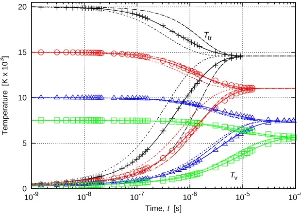
Figure 4. V-T relaxation of an O₂ reservoir from an initial translational-rotational temperature of 20, 000 K,

vibrational temperature of 300 K, and a pressure of 0.063 atm. The crosses are ensemble averages resulting

from DSMC computations. Any solid lines representhy2Foam results using DSMC’sτ_V−T curve-fitted profile.

Any dashed lines and dashed-dotted lines display the results using MW and MWP correlations, respectively.

Other case scenarios have been tested by varying the initial translational-rotational temperature for O₂ (Figure 5(a)) or changing the species to be N2 or NO (Figure5(b)). The initial number density was held

constant and equal to n0_{= 2.282×10}22_m−3_{. Conclusions similar to the previous paragraph can be drawn}

regarding the use of MW correlation and DSMC results to recoverτ_V−T. As for the MWP correlation, the thermal relaxation becomes faster forT0

trno greater than 15,000 K and the specific case of the N2molecule.

More generally MWP is to be prefered to MW for each of these case scenarios.

0 5 10 15 20

10-9 10-8 10-7 10-6 10-5 10-4

Temperature [K x 10

3 ]

Time, t [s]

T

tr

T_v

(a) Molecular temperatures distributions versus time for differentT0 tr

0 5 10 15 20

10-9 10-8 10-7 10-6 10-5

Temperature [K x 10

3 ]

Time, t [s]

O₂

T_tr

T

v N₂

NO

(b) Molecular temperatures distributions versus time for different molecules

Figure 5. V-T relaxation of a heat bath considering several initial translational-rotational temperatures and each of the three molecules composing a five-species air mixture. The symbols are ensemble averages resulting

from DSMC computations. Any solid lines representhy2Foam results using DSMC’sτ_V−T curve-fitted profile.

Any dashed lines and dashed-dotted lines display the results using MW and MWP correlations, respectively.

C. Discussion on the V-T relaxation time

In DSMC computations, the rotational collision number was set to unity to enable a direct comparison between the DSMC and CFD results. Thus, the translational and rotational energy pools were considered to be in thermal equilibrium after a single particle collision event. While this restriction has shown to be very useful to validate the implementation of hy2Foam, a typical value of 5 is usually adopted.15 _{In this}

latter case, the V-T relaxation time will differ from the case Zr = 1 due to rotational-translational and rotational-vibrational energy transfers.

Since no current correlation model can satisfactorily predict case scenarios that depart significantly from weak non-equilibrium conditions, it is thought that the DSMC method could mitigate this gap. Indeed, the determination of the V-T relaxation time from DSMC computations seems to be promising. It has yielded to a very satisfactory agreement for a given set of initial conditions. The question is whether a generalisation to any degree of thermal non-equilibrium is possible.

A preliminary formulation is proposed in Equation 24for a single-species gas. It takes the form of the Millikan-White correlation, corrected by Park, and introduces a series of coefficients Λ to tune accordingly. The vibrational temperature now enters into the calculation of the V-T relaxation time and aims at modelling cases with various degrees of non-equilibrium.

p×τi,V−T =exp "

θ4_v,i/3

r

Mi 2 Λa T

Λb tr + Λc

Mi 2

1/4

+ Λd

Tv,i θv,i

Λe!

+ Λf #

+ Λg ¯ ciσvni

(24)

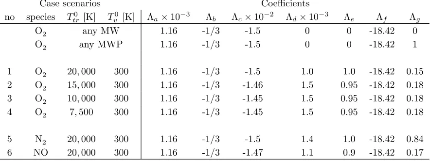
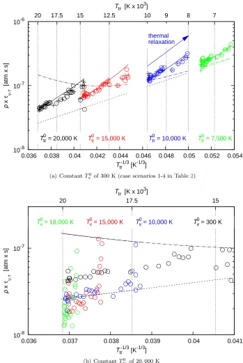
Following Equation24, Table2shows values of the various parameters used to produce the results shown in Figures 3, 4, and 5. Case scenarios 1-4 are reported in Figure 6(a). Kim and Boyd34 _{have performed a}

master equation analysis for N + N₂considering an adiabatic heat bath in strong and weak non-equilibrium conditions. It can be observed that the different profiles of p×τ_V−T versus T_tr−1/3 exhibit a similar trend to those presented in the aforementioned paper. The slope of DSMC best fit (solid line) strongly diverges from both MW and MWP correlations for the greatestT0

tr considered. This slope does not appear to alter significantly as T0

tr decreases. As observed in Table 2, the values of the coefficients Λd and Λe that are responsible for these non-linear profiles appear to be constant for values of T_tr0 no greater than 15,000 K while recalling again thatT_v0 is fixed here to 300 K. Finally,τ_V−T is not appreciably affected by the change

inZrfor the case scenarios that have been investigated.

Table 2. CoefficientsΛfor the evaluation ofτi,V−T in the caseZr= 1

Case scenarios Coefficients

no species T0

tr [K] Tv0[K] Λa×10−3 Λb Λc×10−2 Λd×10−3 Λe Λf Λg

O₂ any MW 1.16 -1/3 -1.5 0 0 -18.42 0

O₂ any MWP 1.16 -1/3 -1.5 0 0 -18.42 1

1 O₂ 20,000 300 1.16 -1/3 -1.5 1.0 1.0 -18.42 0.15

2 O₂ 15,000 300 1.16 -1/3 -1.46 1.5 0.95 -18.42 0.18 3 O₂ 10,000 300 1.16 -1/3 -1.45 1.5 0.95 -18.42 0.18

4 O₂ 7,500 300 1.16 -1/3 -1.45 1.5 0.95 -18.42 0.18

5 N₂ 20,000 300 1.16 -1/3 -1.5 1.4 1.0 -18.42 0.84

6 NO 20,000 300 1.16 -1/3 -1.47 1.1 0.9 -18.42 0.17

In Figure6(b), the influence ofT0

v is highlighted forTtr0 fixed at 20,000 K. It is interesting to note that while MWP is normally employed in high-temperature conditions, MW performs better as T0

v approaches T0

10-8

10-7

10-6

0.036 0.038 0.04 0.042 0.044 0.046 0.048 0.05 0.052 0.054

20 17.5 15 12.5 10 9 8 7

p

x

τ V-T

[atm x s]

T-1/3

tr [K-1/3]

T

tr [K x 10

3

]

thermal relaxation

T0

tr = 20,000 K T0tr = 15,000 K T0tr = 10,000 K T0tr = 7,500 K

(a) ConstantTv0 of 300 K (case scenarios 1-4 in Table2)

10-8

10-7

0.036 0.037 0.038 0.039 0.04 0.041

20 17.5 15

p

x

τ V-T

[atm x s]

T-1/3

tr [K-1/3]

T

tr [K x 10

3

]

T0

v = 18,000 K T0v = 15,000 K T0v = 10,000 K T0v = 300 K

(b) ConstantT0

trof 20,000 K

Figure 6. V-T relaxation time versus T_tr−1/3 for an O₂ adiabatic heat bath with a constant initial number

density of 2.282×1022m−3. The crosses and circles are the ensemble averages resulting from the use of DSMC

data to recover τ_V−T withZr= 1 andZr= 5, respectively. The solid line represents the curve-fitted profile.

The dashed line and dashed-dotted line display the results using MW and MWP correlations, respectively.

It is obvious that a greater diversity of DSMC simulations should be run in order to ascertain noticeable patterns in the evolution of the Λ coefficients. Future work will therefore consist of enlarging the DSMC data set and running a least-squares algorithm to obtain a best-fit. It should be further pointed out that onlyheating case scenarios (T0

IV.

Conclusion

A new open-source CFD solver, hyFoam, has been implemented into the OpenFOAM framework for the prediction of hypersonic reacting flows. The solver has first been validated for a 0-D adiabatic heat bath considering the reversible reaction of hydrogen and iodine I₂+ H₂ −−₎₋₋* 2HI. This work has then been extended to high-temperature conditions with the study of the dissociation of oxygen for several initial temperatures. In comparison with a previously published analytical code, hyFoam is shown to perform equally well. Considering the dissociation reaction of oxygen, the CFD and DSMC results were in satisfactory agreement considering the limitations in the use of a single-temperature CFD model. Efforts have been undertaken to implement the translational/rotational-vibrational energy exchange rate in a two-temperature configuration, to produce a new solver called hy2Foam. hy2Foam has been validated for a 0-D adiabatic heat bath consisting of single-species gases initially set in a state of thermal non-equilibrium.

Future work will consider the generalisation of the two-temperature model to multi-species mixtures and case scenarios with a spatial dimension. A wider range of chemical reactions will be assessed including molecule-molecule and molecule-atom dissociation reactions in a 5-species air mixture composed of O₂, O, N₂, N, and NO.13 _{Further studies will also be carried out in order to assess how the DSMC simulations}

could potentially provide a corrected formulation to the current state-of-the-art CFD V-T relaxation time semi-empirical correlations. This study is the premise to a future open-source hybrid CFD-DSMC solver. In this respect, the work carried out on improving the capabilities of the CFD solver is also important in order to achieve a satisfactory compatibility between the two distinct numerical approaches.

References

1_{Brown, R. E., “The future of air travel: Dinner in Sydney, London in time for ’The X-Factor’ ?” The Washington Post,} Oct. 2014.

2_{Salas, M. D., “A Review of Hypersonics Aerodynamics, Aerothermodynamics and Plasmadynamics Activities within} NASA’s Fundamental Aeronautics Program,” Aiaa 2007-4264, 2007.

3_{Feldick, A. M., Modest, M. F., Levin, D. A., Gnoffo, P., and Johnston, C. O., “Examination of Coupled Continuum Fluid} Dynamics and Radiation in Hypersonic Simulations,”AIAA Aerospace Sciences Meeting, 2009.

4_{Candler, G. V., Write, M. J., and McDonald, J. D., “Data-Parallel Lower-Upper Relaxation Method for Reacting Flows,”} AIAA Journal, Vol. 32, No. 12, 1994, pp. 2380–2386.

5_{Cheatwood, F. M. and Gnoffo, P. A., “User’s Manual for the Langley Aerothermodynamic Upwind Algorithm (LAURA),”} Tech. rep., 1996.

6_{“VULCAN-CFD official website,”http://vulcan-cfd.larc.nasa.gov/, Accessed: 22 May 2015.}

7_{Nompelis, I., Drayna, T. W., and Candler, G. V., “Development of a Hybrid Unstructued Implicit Solver for the Simulation} of Reacting Flows Over Complex Geometries,” Aiaa paper 2004-2227, 2004.

8_{Nompelis, I., Drayna, T. W., and Candler, G. V., “A Parallel Unstructured Implicit Solver for Hypersonic Reacting Flow} Simulation,” Aiaa paper 2005-4867, 2005.

9_{Scalabrin, L. C. and Boyd, I. D., “Development of an Unstructured Navier-Stokes Solver For Hypersonic Nonequilibrium} Aerothermodynamics,” Aiaa paper 2005-5203, June 2005.

10_{Scalabrin, L. C. and Boyd, I. D., “Numerical Simulation of Weakly Ionized Hypersonic Flow for Reentry Configurations,”} Aiaa paper 2006-3773, June 2006.

11_{Park, C., “On Convergence of Computation of Chemically Reacting Flows,”Progress in Astronautics and Aeronautics,} Vol. 103, 1986, pp. 478–513.

12_{“OpenFOAM official website,”http://www.openfoam.com/, Accessed: 22 May 2015.}

13_{Scanlon, T. J. et al., “Open souce Direct Simulation Monte Carlo (DSMC) chemistry modelling for hypersonic flows,”} AIAA Journal, Vol. 53, No. 6, 2015, pp. 1670–1680.

14_{Cassineli Palharini, R.,Atmospheric Reentry Modelling Using an Open-Source DSMC Code, Ph.D. thesis, University of} Strathclyde, Glasgow, 2014.

15_{Bird, G. A.,The DSMC Method, Sydney, 2nd ed., 2013, ISBN : 9781492112907.}

16_{Borgnakke, C. and Larsen, P. S., “Statistical collision model for simulating polyatomic gas with restrited energy exchange,”} Rarefied Gas Dynamics, Vol. 1, 1974, Paper A7, DFVLR Press, Porz-Wahn, Germany.

17_{Greenshields, C. J., Weller, H. G., Gasparini, L., and Reese, J. M., “Implementation of semi-discrete, non-staggered} central schemes in a collocated, polyhedral, finite volume framework, for high-speed viscous flows,”International Journal For Numerical Methods In Fluids, Vol. 63, No. 1, 2010, pp. 1–21.

18_{Kurganov, A., Noelle, S., and Petrova, G., “Semi-discrete central-upwind schemes for hypersonic conservation laws and} Hamilton-Jacobi equations,”SIAM J. Sci. Comput., Vol. 23, No. 3, 2001, pp. 707–740.

19_{Vos, J. B., Rizzi, A., Darracq, D., and Hirschel, E. H., “Navier-Stokes solvers in European aircraft design,”Progress in} Aerospace Sciences, Vol. 38, 2002, pp. 601–697.

21_{Williams, F. A.,Combustion Theory, Addison-Wesley, Redwood City, CA, 2nd ed., 1985.}

22_{Park, C., “Assessment of a Two-Temperature Kinetic Model for Dissociating and Weakly Ionizing Nitrogen,”Journal of} Thermophysics and Heat Transfer, Vol. 2, No. 1, 1988, pp. 8–16.

23_{Born, R. and Oppenheimer, M., “Zur Quantentheorie der Molek¨ule,”Annalen der Physik, Vol. 84, 1941, pp. 457–484.} 24_{Giordano, D., “Impact of the Born-Oppenheimer approximation on aerothermodynamics,” Journal of Thermophysics} and Heat Transfer, Vol. 21, No. 3, 2007, pp. 647–657.

25_{Park, C., Howe, J. T., Jaffe, R. L., and Candler, G. V., “Review of Chemical-Kinetic Problems of Future NASA Missions,} II: Mars Entries,”Journal of Thermophysics and Heat Transfer, Vol. 8, No. 1, 1994, pp. 9–23.

26_{Olynick, D., Taylor, J. C., and Hassan, H. A., “Comparisons Between Monte Carlo Methods and Navier-Stokes Equations} for Re-Entry Flows,”Journal of Thermophysics and Heat Transfer, Vol. 8, No. 2, 1994, pp. 251–258.

27_{Hash, D. et al., “FIRE II Calculations for Hypersonic Nonequilibrium Aerothermodynamics Code Verification: DPLR,} LAURA, US3D, and LeMANS,” Aiaa paper 2007-605, 2007.

28_{Candler, G. V. and Nompelis, I., “Computational Fluid Dynamics for Atmospheric Entry,” Rto-en-avt-162, 2009.} 29_{Laudau, L. and Teller, E., “Theory of sound dispersion,”Physikalische Zeitschrift der Sowjetunion, Vol. 10, 1937.} 30_{Millikan, R. C. and White, D. R., “Systematics of Vibrational Relaxation,”The Journal of Chemical Physics, Vol. 39,} No. 12, 1963, pp. 3209–3213.

31_{Park, C.,Nonequilibrium Hypersonic Aerothermodynamics, Wiley International, New York, 1990.}

32_{Dunn, M. G. and Kang, S. W., “Theoretical and Experimental Studies of Reentry Plasmas,” Nasa cr–2232, April 1973.} 33_{Bussing, T. and Eberhardt, S., “Chemistry Associated with Hypersonic Vehicles,” Aiaa paper 87-1292, 1987.}