Addendum to "A coarse space for heterogeneous Helmholtz problems based on the Dirichlet-to-Neumann operator"' [J. Comput. Appl. Math. 271 (2014) 83–99]

Corrigendum to “A coarse space for heterogeneous

Helmholtz problems based on the Dirichlet-to-Neumann

operator” [J. Comput. Appl. Math. 271 (2014) 83–99]

Lea Conena,∗, Victorita Doleanb, Rolf Krausea, Fr´ed´eric Natafc

a_{Universit`a della Svizzera italiana, Institute of Computational Science, Via G. Buffi 13,}

6900 Lugano, Switzerland

b_{University of Strathclyde, Dept. of Mathematics and Statistics, 26 Richmond Street,}

Glasgow G1 1XH, Scotland, UK

c_{Universit´e Pierre et Marie Curie, Laboratoire J.L. Lions, Tour 15-25 Bureau 319, 4 place}

Jussieu, 75005 Paris, France

Abstract

This communication gives a corrigendum to the paper “A coarse space for het-erogeneous Helmholtz problems based on the Dirichlet-to-Neumann operator” [J. Comput. Appl. Math. 271 (2014) 83–99].

Keywords: Helmholtz equation, domain decomposition, coarse space, Dirichlet-to-Neumann operator

The preconditioner

PBNN=QM−1P+ZE−1Y† (1) from [1, Equation (7)] might be singular for general non-singular matrices A,

M andE=YTAZ, and full ranked matricesZ andY. Consider

A=





2 5 2

0 6 0

0 1 4



, Z =Y = 



0 1 1



, M−1= 



1 1 0

1 0 0

0 0 1



.

The matricesA, M, and E are clearly non-singular, but 15 −4 7T

is an eigenvector of PBA with eigenvalue 0. This is in contradiction to a result of Erlangga and Nabben [2], on which our work was based. Their consequently wrong theorem reads

Theorem 0.1 ([2, Theorem 2.9]). Let Z andY be full ranked. LetM be non-singular. Then PBNNA is non-singular. In addition, any zero eigenvalue of

M−1_P

DA is shifted to one inPBNNA.

∗_{Corresponding author. Phone number: +41 (0)58 666 4975}

Email addresses: [email protected](Lea Conen),[email protected]

0 50 100 150 0 50 100 150 nloc Num b er of iterations

(a) Number of iterations

Crit. 4.3 2 extra modes negative

0 50 100 150

0 200 400 600 nloc Dimension of coarse space

(b) Dimension of the coarse space

Figure 5: Comparison of different criteria of how many DtN modes to choose.

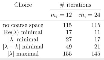
Choice # iterations

mi = 12 mi= 24

no coarse space 115 115

Re(λ) minimal 17 11

|λ|minimal 27 17

|λ−k|minimal 49 21

|λ| maximal 155 145

Table 1: Iteration numbers for different choices of DtN eigenfunctions.

The solutions of the preconditioned of the original system might hence dif-fer and the GMRES solver employed in [1] is not adapted to solve systems with singularities. For that reason, in this corrigendum the results of [1] are reproduced using a non-singular preconditioner. Numbering and notation are identitical to the original paper. The new results use the provably non-singular preconditioner [3]

Pnew =I−Z Z†M−1AZ −1

Z†M−1A+Z Z†M−1AZ−1Z† (2) and solve the preconditioned problemM−1_AP

new =M−1b. The coarse matrix is nowZ†_M−1_{AZ instead ofZ}†_{AZin Equation (1). Its sparsity structure hence} changes; it has blocks not only for neighboring subdomains but also for neighbors of neighbors, which constitutes a drawback for parallel implemetation.

We make a few observations, refraining however from giving a detailed in-terpretation of the new results to save space. The eigenvalue distribution in Figure 7a is more favorable than the one forPBNNA. This is also reflected in the iteration counts for small coarse size, see e.g. Figure 6 or the last line of Table 14 for PW 10−2

L k kL # iterations coarse space dimension

1 30 30 20 224

5 6 30 20 224

10 3 30 19 224

Table 2: Dependence on the sizeLof the domain Ω = [0, L]2_.

0 5 10 15

0 20 40 60 80

Number of modesmi

Num b er of iterations 1-level DtN

Figure 6: Number of iterations in dependence ofmi.

M-1_{A M}−1_AP new

−1−0.5 0 0.5 1 −1

0 1

(a)mi= 2

−1−0.5 0 0.5 1 −1

0 1

(b)mi= 16

Figure 7: 100 largest eigenvalues for I−M−1_AandI− M−1_{APnewin the complex plane.}

nloc k 1-lev DtN PW(10−2) PW(10−1)

20 18.5 80 16 (144) − (352) 9 (293)

40 29.3 116 19 (224) − (467) 13 (382)

80 46.5 156 30 (299) − (577) 16 (505)

160 73.8 217 40 (508) − (609) 25 (597)

Table 3: Number of iterations (dimension of coarse space).

k3_h2_{= 1 k}3_h2₌2π

10 k

3_h2_{= 0.1}

20 40 60 80

10 20 30 40 50 k n um b er of iterations

20 40 60 80

200 400 k coarse space dimension

mi from DtN coarse space mi from PW coarse space

nloc k mi DtN PW(10−2) PW(10−1) mi DtN PW(10−2) PW(10−1)

10 11.6 4 15 17 (100) 17 (100) 12 8 7 (288) 7 (244)

20 18.5 6 19 19 (150) 19 (146) 15 9 − (355) 9 (305)

40 29.3 9 23 22 (225) 22 (225) 17 13 − (409) 13 (373)

80 46.5 12 35 30 (296) 29 (292) 24 19 − (556) 16 (496)

160 73.8 21 42 − (521) 31 (513) 25 39 − (609) 25 (597)

Table 4: Comparison of number of iterations with identical coarse space size for DtN and PW.

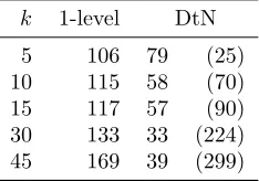
k 1-level DtN

5 106 79 (25)

10 115 58 (70)

15 117 57 (90)

30 133 33 (224)

45 169 39 (299)

Table 5: Dependence on wave number for fixed mesh width.

we additionally give results for PW 10−1

. In total, the results do not change substantially and the conclusions drawn in [1] remain valid.

References

[1] L. Conen, V. Dolean, R. Krause, F. Nataf, A coarse space for heteroge-neous Helmholtz problems based on the Dirichlet-to-Neumann operator, J. Comput. Appl. Math. 271 (2014) 83 – 99.

[2] Y. A. Erlangga, R. Nabben, Deflation and balancing preconditioners for Krylov subspace methods applied to nonsymmetric matrices, SIAM J. Ma-trix Anal. Appl. 30 (2008) 684–699.

[3] P. Hav´e, R. Masson, F. Nataf, M. Szydlarski, H. Xiang, T. Zhao, Algebraic

nloc= 20,L= 2 nloc= 80,L= 2 nloc= 80,L= 8

k 1-level DtN 1-level DtN 1-level DtN

1 73 51 (25) 94 73 (25) 66 46 (25)

5 64 40 (25) 96 70 (25) 55 34 (25)

10 68 24 (74) 106 47 (74) 66 24 (74)

20 84 22 (139) 107 34 (144) 86 21 (139)

Number of subdomains

nloc k 5×5 5×10 5×20 5×40

10 11.6 16 (80) 18 (180) 21 (380) 24 (780)

20 18.5 16 (144) 18 (314) 19 (654) 21 (1334)

40 29.3 20 (224) 20 (484) 22 (1004) 24 (2044) 80 46.5 31 (299) 37 (644) 45 (1334)

Table 7: Dependence on number of subdomains, DtN coarse space.

DtN PW(10−2) PW(10−1)

# subdomains # it. size # it. size # it. size

2×2 24 (68) − (96) 18 (88)

4×4 31 (200) − (368) 15 (320)

8×8 40 (416) − (1116) 14 (924)

16×16 60 (960) − (3256) 12 (2686)

32×32 48 (2944) ? (9208) ? (?)

Table 8: Second scaling test: Vary the number of subdomains.

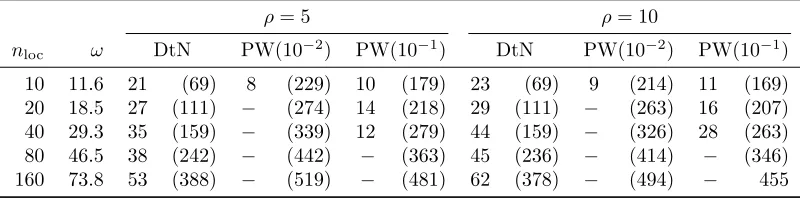
ρ= 5 ρ= 10

nloc ω DtN PW(10−2) PW(10−1) DtN PW(10−2) PW(10−1)

10 11.6 21 (69) 8 (229) 10 (179) 23 (69) 9 (214) 11 (169)

20 18.5 27 (111) − (274) 14 (218) 29 (111) − (263) 16 (207)

40 29.3 35 (159) − (339) 12 (279) 44 (159) − (326) 28 (263)

80 46.5 38 (242) − (442) − (363) 45 (236) − (414) − (346)

160 73.8 53 (388) − (519) − (481) 62 (378) − (494) − 455

Table 9: Number of iterations (coarse space dimension) for heterogeneous open cavity problem.

ρ 1-level DtN PW(10−2) PW(10−1)

100 156 31 (299) − (577) 16 (505)

101 154 45 (236) − (414) − (346)

102 173 59 (236) − (388) − (320)

103 177 64 (236) − (379) − (315)

nloc ω mi DtN PW(10−2) PW(10−1)

10 11.6 3 21 22 (75) 22 (75)

20 18.5 5 23 25 (123) 25 (123)

40 29.3 7 38 40 (171) 41 (163)

80 46.5 10 42 − (237) 45 (223)

160 73.8 16 59 − (358) 63 (346)

Table 11: Fixed coarse space size for heterogeneous open cavity problem.

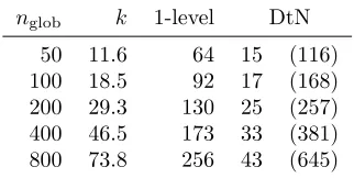
nglob k 1-level DtN

50 11.6 64 15 (116)

100 18.5 92 17 (168)

200 29.3 130 25 (257)

400 46.5 173 33 (381)

800 73.8 256 43 (645)

Table 12: Decomposition with Metis.

5×5 subdomains 10×10 subdomains

k nglob DtN PW(10−2) PW(10−1) DtN PW(10−2) PW(10−1)

18.5 100 15 (144) 8 (355) 9 (293) 17 (364) 23 (1152) 8 (872)

29.3 200 18 (224) − (466) 13 (379) 22 (460) − (1288) 11 (1132)

46.5 400 27 (315) − (577) 16 (511) 35 (660) − (1712) 15 (1380)

73.8 800 33 (514) − (609) 25 (597) 57 (956) − (2346) 18 (1928)

Table 13: Number of iterations (coarse space dimension) for Problem 2.

15 subdomains 60 subdomains

ω n DtN PW(10−2) PW(10−1) DtN PW(10−2) PW(10−1)

90 150×250 14 (267) 12 (346) 12 (323) 21 (541) 10 (1038) 12 (877)

180 300×500 15 (514) 24 (375) 24 (373) 22 (1074) 15 (1426) 15 (1333)

360 600×1000 18 (968) 50 (375) 50 (375) 26 (2113) 42 (1500) 42 (1500)