An exact dynamic stiffness element using a higher order shear deformation theory for free vibration analysis of composite plate assemblies

(1)

City, University of London Institutional Repository

Citation

:

Fazzolari, F. A., Boscolo, M. and Banerjee, J. R. (2013). An exact dynamic

stiffness element using a higher order shear deformation theory for free vibration analysis of

composite plate assemblies. Composite Structures, 96, pp. 262-278. doi:

10.1016/j.compstruct.2012.08.033

This is the accepted version of the paper.

This version of the publication may differ from the final published

version.

Permanent repository link:

http://openaccess.city.ac.uk/14986/

Link to published version

:

http://dx.doi.org/10.1016/j.compstruct.2012.08.033

Copyright and reuse:

City Research Online aims to make research

outputs of City, University of London available to a wider audience.

Copyright and Moral Rights remain with the author(s) and/or copyright

holders. URLs from City Research Online may be freely distributed and

linked to.

City Research Online: http://openaccess.city.ac.uk/ [email protected]

(2)

An Exact Dynamic Stiffness Element Using a Higher Order

Shear Deformation Theory for Free Vibration Analysis of

Composite Plate Assemblies

F. A. Fazzolari1,_∗_{, M. Boscolo}2_{, J. R. Banerjee}3

City University London, Northampton Square, London, EC1V 0HB, United Kingdom

Abstract

An exact dynamic stiffness method based on higher order shear deformation theory is developed for the

first time using symbolic computation in order to carry out free vibration analysis of composite plate

assemblies. Hamilton’s principle is applied to derive the governing differential equations of motion and

natural boundary conditions. Then by imposing the geometric boundary conditions in algebraic form the

dynamic stiffness matrix is developed. The Wittrick-Williams algorithm is used as solution technique to

compute the natural frequencies and mode shapes for a range of laminated composite plates and stepped

panels. The effects of significant parameters such as thickness ratio, orthotropy ratio, step ratio, number

of layers, lay-up and stacking sequence and boundary conditions on the natural frequencies and mode

shapes are critically examined and discussed. The accuracy of the method is demonstrated by comparing

results with those available in the literature.

Keywords: Dynamic Stiffness Method, Composite Plates, Free Vibration, Stepped Panels,

Wittrick-Williams algorithm.

1. Introduction

During the last three decades thin-walled composite structures have played very important roles in

aerospace, automotive, marine and civil engineering design, amongst many others. The use of advanced

composite materials allows structures to be much stiffer and stronger and yet much lighter. When these

materials are combined with cutting-edges manufacturing technologies, they provide design engineers a

competitive edge over conventional design with metallic construction. For this reason, research in the

static and dynamic behavior of composite structures has continued to grow. In particular, free vibration

analysis of assemblies of composite plates has received wide attention over the years. The research is

further stimulated by the fact that many practical structural components can be modelled adequately

as thin or thick metallic or composite plates. One method of analysis, other than the conventional finite

element method (FEM) for this type of structures is that of the dynamic stiffness method (DSM) (see

∗_{Corresponding author: Tel:+44(0)2070400224, Fax:+44(0)2070408566}

Email address: [email protected](F. A. Fazzolari)

1

PhD Candidate, School of Engineering and Mathematical Sciences

2

Researcher Fellow, School of Engineering and Mathematical Sciences

3

(3)

[1]). Application of this method involves developing the dynamic stiffness (DS) matrix for each individual

element in the structure and then assembling them into a global DS matrix for subsequent free vibration

analysis. This method is, in many ways, analogous to the conventional finite element method (see [2]).

The main difference between the two methods is that the FEM discretizes a structural element based on

assumed shape functions to derive the mass and stiffness matrices separately, whereas the DSM uses a

single element matrix containing both mass and stiffness proprieties, which are derived from the exact

frequency-dependent shape functions obtained from the solution of the governing differential equations

of the element in free vibration. The assembly procedure for the two methods is essentially the same,

but the solution techniques are different in that the FEM generally leads to a linear eingenvalue problem

in sharp contrast to the non-linear (transcendental) eigen-solution encountered in the DSM, which is

generally solved by applying the well-established algorithm of Wittrick and Williams [3]. For structures

consisting of beam elements there is no restriction on the application of the DSM and there are some well

known software based on the method to analyze plane or space frames [4]. Another important difference

between the FEM and the DSM is that, the number of natural frequencies that can be computed using the

FEM is restricted to the number of chosen degrees of freedom of the structure and the accuracy of results

diminishes with higher order modes. This can be a serious limitation in modal analysis. By contrast,

the DSM has no such limitation and any number of natural frequencies can be computed to any desired

accuracy using the DS matrix without the need to increase the number of elements to achieve higher

accuracy. Moreover, when fast iterative matrix solvers are used, the DSM will be much more efficient

than the FEM. With regard to plate elements the DSM gives exact results because the equations of motion

are solved in L`evy-type closed form to obtain the element properties and no other approximation is made

en route during the analysis. Wittrick and Williams [5] are known to be the first who attempted the

extension of DSM to plate elements. Their pioneering formulation is interesting and relies on extensive

use of complex algebra. In 1972, Williams [6] presented two computer programs, GASVIP and VIPAL

to compute the natural frequencies, based on DSM. Essentially GASVIP was used to set up the overall

stiffness matrix for the structure, and VIPAL demonstrated the use of substructuring. A couple of

years later, Wittrick and Williams reported the computer code VIPASA [5] for free vibration analysis

of prismatic plate assemblies, which was a significant development at the time. VIPASA code allowed

free vibration analysis of isotropic or anisotropic plates and had many additional features. The complex

stiffnesses described in [7] were incorporated, as well as allowances for eccentric connections between

the component plates were accounted for, but more importantly, the code used a powerful algorithm

as solution technique, developed by Wittrick and Williams [3] to compute natural frequencies of plated

structures. The algorithm is robust and it ensures that no natural frequencies of the structure are missed.

(A brief discussion of the Wittrick-Williams algorithm is presented in section (2.5)). In 1983, Williams

and Anderson [8] showed modifications to the eigenvalue algorithm described in [3]. They made use of

Lagrangian multipliers to apply point constraints at any location of plate edges. Each sinusoidal mode of

the freely vibrating plate in the longitudinal direction was included within the dynamic stiffness matrix.

These modifications formed the basis for the enhanced computer code VICON (VIpasa with CONstraints)

(4)

of VICON was based on classical plate theory (CPT), and particularly for composite plates, attention

was focused on symmetric laminates. A later version of the code included plates on Winkler foundations

[10]. Next, a major enhancement of the program took place in the early nineties when the optimum

design features were added and the new program VICONOPT (VICON with OPTimization) [11, 12] was

born. Anderson and Kennedy [13] incorporated the effect of the shear deformation into VICONOPT

few years later using a numerical approach. The general purpose application of VICONOPT was further

enhanced by them [13] to allow for analysis of angle-ply laminates. An interesting historical review of

the DSM procedure for plates can be found in [14]. It should be noted that DSM has been extensively

researched by Banerjee [1, 15, 16, 17, 18, 19], amongst others for modal analysis of structures idealized

by beam elements based on Euler-Bernoulli, Timoshenko and associated coupled beam theories. The

extension of the DSM to plate elements is no-doubt difficult, but indeed, essential to model complex

structures. Following the earlier research on DS theories of isotropic and composite plates, Boscolo and

Banerjee advanced the state of the art on these topics by including the effects of shear deformation and

rotatory inertia and thereby providing a detailed modal analysis procedure through the application of

symbolic computation and Matlab [20, 21, 22, 23]. They used the first order shear deformation theory

(FSDT) for which the introduction of a user specified shear corrector factor was necessary. The current

paper is partly motivated by these earlier developments and the most important contribution made by

the authors here is the inclusion of higher order shear deformation theory (HSDT), for the first time,

when developing the DS matrix for laminated composite plates. This useful extension is of considerable

theoretical and computational complexity as will be shown later. The research is particularly relevant

when analysing thick composite plates for their free vibration characteristics. It should be recognised

that Reddy and co-authors [24, 25, 26] have used HSDT in a different context in free vibration analysis

of composite plates without resorting to the development of the DSM. From a historical prospective

HSDT, can be traced back to third order plate bending theory originally proposed by Vlasov [27] in

the late fifties. His theory was substantiated and extended to laminated composite plates many years

later by Reddy [24] using a variational approach. This is sometimes referred to as Vlasov-Reddy theory

(VRT). Further improvements of this theory can be found in the work of Jemielita [28, 29]. During the

last two decades, a variable kinematics 2D model approach with hierarchical capabilities, particularly

for laminated composite beams, plates and shells, has been proposed by Carrera et al. for mechanical

[30, 31, 32, 33, 34] and multifield [35, 36, 37] problems. Inclusion of HSDT in the DSM framework will

enable free vibration analysis of plates with moderate to high thickness to width ratio, in an accurate

and computationally efficient manner. One of the great advantages of using HSDT as opposed to FSDT

is that the former accounts for the effects of the shear deformation in a judicious manner without using

a fictitious (and often controversial) shear correction or shape factor that is prevalent in the latter.

The usefulness of HSDT becomes apparent when analysing composite structures, particularly of thicker

dimensions, because fiber reinforced composites have generally very low shear modulii. Both the in-plane

and out-of-plane free vibration analyses are considered in this paper. Extensive results which include

validation and assessment of the effects of significant parameters such as the thickness to width (or

(5)

have been computed and discussed. The paper finished with some concluding remarks.

2. Theoretical formulation

2.1. Displacement field and governing differential equations

In the derivation that follows, the hypotheses of straightness and normality of a transverse normal after

deformation are assumed to be no longer valid for the displacement field which is now considered to be

a cubic function in the thickness coordinate; and hence the use of higher order shear deformation theory

(HSDT). This is in sharp contrast to earlier formulations based on CPT and FSDT. For a composite

plate, the kinematics of deformation of a transverse normal using both first order and higher order shear

deformation are schematically shown in Fig. 1. The laminate is assumed to be composed ofNllayers so

that the theory is sufficiently general. The integerk is used as a superscript denoting the layer number

where the numbering starts from the bottom. After imposing the transverse shear stress homogeneous

conditions [38, 39] at the top/bottom surface of the plate, the displacements field is given below in the

usual form:

u(x, y, z, t) = u0(x, y, t) +z φx(x, y, t)−z3 4 3h2

φx+

∂w0 ∂x

v(x, y, z, t) = v0(x, y, t) +z φy(x, y, t)−z3 4 3h2

φy+

∂w0 ∂y

w(x, y, z, t) = w0(x, y, t)

(1)

whereu,v,ware general displacements within the plate in the x, y, and z directions, respectively, whereas

u0,v0,w0are the corresponding displacements of the reference surface (mid-plane Ω). Hamilton principle

is now applied. The variational statement is:

Nl

X

k=1

Z t2

t1

δ_Lk_dt_{= 0} ₍₂₎

where_Lk _{is the Lagrangian for the kth layer of the composite plate. The first variation can be expressed}

as:

δLk₌_δTk

−δUk ₍₃₎

where δUk _{is the virtual strain energy,}_δTk _{is the virtual kinetic energy, and assume the following form:}

δUk ₌Z Ωk

Z

zk

δεkTσkdΩk_dz

δTk ₌Z Ωk

Z

zk ρk_δ

ηTη¨

dΩk_dz

(4)

the stresses (σ), the strains (ε) and the displacements (η) vectors are expressed as follows:

σ=n σxx σyy σxy σxz σyz

oT

ε=n εxx εyy γxy γxz γyz

oT

η=n u v w

oT

(6)

ρk _{denotes mass density while an over dot denotes differentiation with respect to time. The subscript}_T

signifies an array transposition andδthe variational operator. Constitutive and geometrical relationships

(deformation) are respectively defined as:

σk_{= ˜}_Ck_εk_, _ε₌

Dη (6)

where ˜Ck is the plane stress constitutive matrix and D is the differential matrix (see Appendix A for

details). Substituting Eq. (6) into the Eq. (4) and imposing the condition in Eq. (2), the equations of

motion are obtained after extensive algebraic manipulation as:

δu0: A11u0,xx+A12v0,yx+A16(u0,yx+v0,xx) +B11φx,xx+B12φy,yx+B16(φx,yx+φy,xx) +E11c2φx,xx

+E11c2w0,xxx+E12c2φy,yx+E12c2w0,yyx+E16c2φx,yx+E16c2φy,xx+ 2E16c2w0,xyx+A16u0,xy

+A26v0,yy+A66(u0,yy+v0,xy) +B16φx,xy+B26φy,yy+B66(φx,yy+φy,xy) +E12c2 (φx,xy+w0,xxy)

+E26c2 (φy,yy+w0,yyy) +E66c2(φx,yy+φy,xy+ 2w0,xyy) =I0u¨0+I1φ¨x+I3c2φ¨x+I3c2w¨0,x

δv0: A16u0,xx+A26v0,yx+A66(u0,yx+v0,xx) +B16φx,xx+B26φy,yx+B66(φx,yx+φy,xx) +E16c2φx,xx

+E16c2w0,xxx+E26c2φy,yx+E26c2w0,yyx+E66c2φx,yx+E66c2φy,xx+ 2E66c2w0,xyx+A12u0,xy

+A22v0,yy+A26(u0,yy+v0,xy) +B12φx,xy+B22φy,yy+B26(φx,yy+φy,xy) +E12c2 (φx,xy+w0,xxy)

+E22c2 (φy,yy+w0,yyy) +E26c2(φx,yy+φy,xy+ 2w0,xyy) =I0v¨0+I1φ¨y+I3c2φ¨y+I3c2w¨0,y

δw0: A44(φy,y+w0,yy) +A45(φx,y+w0,xy) +D44c1(φy,y+w0,yy) +D45c1(φx,y+w0,xy)

+A45(φy,x+w0,xy) +A55(φx,x+w0,xx) +D45c1(φy,x+w0,xy) +D55c1(φx,x+w0,xx)

+D44c1(φy,y+w0,yy) +D45c1(φx,y+w0,xy) +F44c 2

1(φy,y+w0,yy) +F45c 2

1(φx,y+w0,xy)

+D45c1(φy,x+w0,xy) +D55c1(φx,x+w0,xx) +F45c 2

1(φy,x+w0,xy) +F55c 2

1(φx,x+w0,xx)

−E11c2u0,xxx−E12c2v0,xxy−E16c2(u0,xxy+v0,xxx)−F11c2φx,xxx−F12c2φy,xxy

−F16c2(φx,xxy+φy,xxx)−H11c 2

2(φx,xxx+w0,xxxx)−H12c 2

2(φx,xxy+w0,xxyy)

−H16c 2

2(φx,xxy+φy,xxx+ 2w0,xxxy)−2E16c2u0,xxy−2E26c2v0,xyy−2E66c2(u0,xyy+v0,xxy)

−2F16c2φx,xxy−2F26c2φy,xyy−2F66c2(φx,xyy+φy,xxy)−2H16c 2

2(φx,xxy+w0,xxxy)

−2H26c 2

2(φy,xyy+w0,xyyy)−2H66c 2

2(φx,xyy+φy,xxy+ 2w0,xxyy)−E12c2u0,xyy−E22c2v0,yyy

−E26c2(u0,yyy+v0,xyy)−F12c2φx,xyy−F22c2φy,yyy−F26c2(φx,yyy+φy,xyy)

−H12c 2

2(φx,xyy+w0,xxyy)−H22c 2

2(φy,yyy+w0,yyyy)−2H26c 2

2(φx,yyy+φy,xyy+ 2w0,xyyy)

=I0w¨0−I6c 2

2( ¨w0,xx+ ¨w0,yy)−I3c 2

2(¨u0,x+ ¨u0,y)−(I4+I6) c 2 2

¨

φx,x+ ¨φy,y

(7)

δφx: B11u0,xx+B12v0,yx+B16(u0,yx+v0,xx) +D11φx,xx+D12φy,xy+D16(φx,yx+φy,xx)

+F11c2(φx,xx+w0,xxx) +F12c2(φy,yx+w0,yyx) +F16c2(φx,yx+φy,xx+ 2w0,xyx)

+B16u0,xy+B26v0,yy+B66(u0,yy+v0,xy) +D16φx,xy+D26φy,yy+D66 (φx,yy+φy,xy)

+F16c2(φx,xy+w0,xxy) +F26c2(φy,yy+w0,yyy) +F66c2(φx,yy+φy,xy+ 2w0,xyy)

+E11c2u0,xx+E12c2v0,yx+E16c2(u0,yx+v0,xx) +F11c2φx,xx+F12c2φy,xy+F16c2(φx,yx+φy,xx)

+H11c 2

2(φx,xx+w0,xxx) +H12c 2

2(φy,yx+w0,yyx) +H16c 2

2(φx,yx+φy,xx+ 2w0,xyx)

+E16c2u0,xy+E26c2v0,yy+E66c2(u0,yy+v0,xy) +F16c2φx,xy+F26c2φy,yy+F66c2(φx,yy+φy,xy)

+H16c 2

2(φx,xy+w0,xxy) +H26c 2

2(φy,yy+w0,yyy) +H66c 2

2(φx,yy+φy,xy+ 2w0,xyy)

−A45(φy+ 2w0,y)−A55(φx+ 2w0,x)−2D45c1(φy+ 2w0,y)−2D55c1(φx+ 2w0,x)

−F45c 2

1(φy+ 2w0,y)−F55c 2

1(φx+ 2w0,x) = (I1+ c2I3) ¨u0+ I2+ 2 c2I4+ c 2 2I6

_¨

φx+ I4+ c 2 2I6

¨

w0,x

δφy: B16u0,xx+B26v0,yx+B66 (u0,yx+v0,xx) +D16φx,xx+D26φy,xy+D66(φx,yx+φy,xx)

+F16c2 (φx,xx+w0,xxx) +F26c2(φy,yx+w0,yyx) +F66c2(φx,yx+φy,xx+ 2w0,xyx)

+B12u0,xy+B22v0,yy+B26(u0,yy+v0,xy) +D12φx,xy+D22φy,yy+D26(φx,yy+φy,xy)

+F12c2 (φx,xy+w0,xxy) +F22c2(φy,yy+w0,yyy) +F26c2(φx,yy+φy,xy+ 2w0,xyy)

+E16c2u0,xx+E26c2v0,yx+E66c2(u0,yx+v0,xx) +F16c2φx,xx+F26c2φy,xy+F66c2(φx,yx+φy,xx)

+H16c 2

2(φx,xx+w0,xxx) +H26c 2

2(φy,yx+w0,yyx) +H66c 2

2(φx,yx+φy,xx+ 2w0,xyx)

+E12c2u0,xy+E22c2v0,yy+E26c2(u0,yy+v0,xy) +F12c2φx,xy+F22c2φy,yy+F26c2(φx,yy+φy,xy)

+H12c 2

2(φx,xy+w0,xxy) +H22c 2

2(φy,yy+w0,yyy) +H26c 2

2(φx,yy+φy,xy+ 2w0,xyy)

−A44(φy+ 2w0,y)−A45(φx+ 2w0,x)−2D44c1(φy+ 2w0,y)−2D45c1(φx+ 2w0,x)

−F44c 2

1(φy+ 2w0,y)−F45c 2

1(φx+ 2w0,x) = (I1+ c2I3) ¨v0+ I2+ 2 c2I4+ c 2

2I6φ¨y+ I4+ c 2

2I6w¨0,y

(7)

The natural boundary conditions are:

δu0: Nxx=A11u0,x+B11φx,x+E11c2φx,x+E11c2w0,xx+A12v0,y+B12φy,y+E12c2φy,y+E12c2w0,yy

+A16u0,y+A16v0,x+B16φx,y+B16φy,x+E16c2φx,y+E16c2φy,x+ 2E16c2w0,xy

δv0: Nxy=A16u0,x+B16φx,x+E16c2φx,x+E16c2w0,xx+A26v0,y+B26φy,y+E26c2φy,y+E26c2w0,yy

(8)

δw0 : Qx=H11c 2

2φx,xx+H11c 2

2w0,xxx+E11c2u0,xx+F11c2φx,xx+E12c2v0,yx+F12c2φy,yx

+H12c 2

2φy,yx+H12c 2

2w0,yyx+ 2E16c2u0,xy+ 2F16c2φx,xy+ 2H16c 2

2φx,xy+E16c2u0,yx

+E16c2v0,xx+F16c2φx,yx+H16c 2

2φx,yx+H16c 2

2φy,xx+ 2H16c 2

2w0,xxy+ 2E26c2v0,yy

+ 2F26c2φy,yy+ 2H26c 2

2w0,yyy+ 4H66c 2

2w0,xyy+ 2H26c 2

2φx,yy+ 2H26c 2

2φy,xy+ 2E66c2u0,yy

+ 2E66c2v0,xy+ 2F66c2φx,yy+ 2F66c2φy,xy−2D45c1φy−2D45c1w0,y−F45c 2 1φy

−F45c 2

1w0,y−A55φx−A55w0,x−D55c1φx−2 c1w0,x−F55c 2

1φx−F55c 2 1w0,x

δφx: Mxx=D11φx,x+H11c 2

2φx,x+H11c 2

2w0,xx+B11u0,x+E11c2u0,x+ 2F11c2φx,x+F11c2w0,xx

+F11c2w0,xx+B12v0,y+D12φy,y+F12c2φy,y+F12c2w0,yy+E12c2v0,y+F12c2φy,y+H12c 2 2φy,y

+H12c 2

2w0,yy+B16u0,y+B16v0,x+D16φx,y+D16φy,x+F16c2φx,y+F16c2φy,x+ 2F16c2w0,xy

+E16c2u0,y+E16c2v0,x+F16c2φx,y+F16c2φy,x+H16c 2

2φx,y+H16c 2

2φy,x+ 2H16c 2 2w0,xy

δφy: Mxy=D16φx,x+H16c 2

2φx,x+H16c 2

2w0,xx+B16u0,x+E16c2u0,x+ 2F16c2φx,x+F16c2w0,xx

+F16c2w0,xx+B26v0,y+D12φy,y+F26c2φy,y+F26c2w0,yy+E26c2v0,y+F26c2φy,y+H26c 2 2φy,y

+H26c 2

2w0,yy+B66u0,y+B66v0,x+D66φx,y+D66φy,x+F66c2φx,y+F66c2φy,x+ 2F66c2w0,xy

+E66c2u0,y+E66c2v0,x+F66c2φx,y+F66c2φy,x+H66c 2

2φx,y+H66c 2

2φy,x+ 2H66c 2 2w0,xy

δw0,x: Pxx=H11c 2

2φx,x+H11c 2

2w0,xx+E11c2u0,x+F11c2φx,x+E12c2v0,y+F12c2φy,y+H12c 2 2φy,y

+H12c 2

2w0,yy+E16c2u0,y+E16c2v0,x+F16c2φx,y+F16c2φy,x+H16c 2

2φx,y+H16c 2 2φy,x

+ 2H16c 2 2w0,xy

(8)

where the suffix after the comma denotes the partial derivative with respect to that variable, and

(Aij, Bij, Dij, Eij, Fij, Hij) = Nl X k=1 Z zk ˜

Cijk 1 z, z 2

, z3, z4, z6

dz

(I0, I1, I2, I3, I4, I6) = Nl

X

k=1

Z

zk

ρk 1z, z2, z3, z4, z6

dz

(9)

are laminate stiffnesses and inertia terms, respectively withiandj varying form 1 to 6.

2.2. Dynamic stiffness formulation

Once the equations of motion and the natural boundary conditions, i.e., Eqs. (7) and (8) are obtained,

the classical method to carry out exact free vibration analysis of a plate consists of (i) solving the system

of differential equations in Navier or L`evy type closed form in an exact manner, (ii) applying particular

boundary conditions on the edges and finally (iii) obtaining the frequency equation by eliminating the

integration constants [40, 41, 42, 43]. This method, although extremely useful for analysing an individual

plate, it lacks generality and cannot be easily applied to complex structures for which researchers usually

resort to approximate methods such as the FEM. In this respect, the dynamic stiffness method (DSM),

(9)

when it is applied to complex structures. The dynamic stiffness matrix of a structural element used in the

DSM has many other advantages. It can be offset and/or rotated and assembled in a global DS matrix

in the same way as the FEM. This global DS matrix contains implicitly all the exact natural frequencies

of the structure which can be computed by using the well established algorithm of Wittrick and Williams

[3].

A general procedure to develop the dynamic stiffness matrix of a structural element can be summarized

as follows:

(i) Seek a closed form analytical solution of the governing differential equations of motion of the

structural element undergoing free vibration.

(ii) Apply a number of general boundary conditions in algebraic forms that are equal to twice the

number of integration constants; these are usually nodal displacements and forces.

(iii) Eliminate the constants by relating the amplitudes of the harmonically varying nodal forces to those

of the corresponding displacements which essentially generates the frequency-dependent dynamic

stiffness matrix, providing the force-displacement relationship between nodes.

Referring to the equations of motions given by Eqs. (7), an exact solution can be sought in L`evy’s form

for symmetric, cross ply laminates. For such laminates B=E = 0,and ˜Ck

16= ˜C26k = ˜C45k = 0 and the

out-of-plane displacements are uncoupled from the in-plane ones.

2.3. L`evy-type closed form exact solution and DS formulation

The solution of Eqs.(7) is sought as:

u0

(x, y, t) =

∞

X

m=1

Um(x) eiωtsin(α y), v 0

(x, y, t) =

∞

X

m=1

Vm(x) eiωtcos(α y),

w0

(x, y, t) =

∞

X

m=1

Wm(x) eiωtsin(α y), φx(x, y, t) = ∞

X

m=1

Φxm(x) e

iωt_sin(_{α y}₎_,

φy(x, y, t) = ∞

X

m=1

Φym(x) e iωt

cos(α y)

(10)

whereωis the unknown circular frequency,α= m π

L andm= 1,2, . . . ,∞. This is the called L`evy’s so-lution which assumes that two the opposite sides of the plate are simply supported (S-S), i.e. w=φx= 0 at y= 0 andy=L. Substituting Eq. (10) into Eqs. (7) a set of five ordinary differential equations that are uncoupled between in-plane and out-of-plane deformations, is obtained which can be written in two different matrix forms as follows:





Lp11 Lp12

Lp21 Lp22

    Um Vm   =   0 0  ,     

Lo11 Lo12 Lo13

Lo21 Lo22 Lo23

Lo31 Lo32 Lo33

          Wm Φx Φy      =      0 0 0      (11)

(10)

case,_Lpij (i, j= 1,2) are given by:

Lp11 = (A66α

2

−I0ω2)−A11Dx2

Lp12 = (A12+A66)αDx

Lp21 = (A12+A66)αDx

Lp22 = (−A22α

2₊_I

0ω2) +A66D2x

(12)

For the out-of-plane case,Loij (i, j= 1,2,3) are given by:

Lo11 = −α

2₍_A

44+ 2c2D44+c22F44+α2c21H22) + (I0+α2c21I6)ω2+ (A55+ 2c1D55+c21F55

+ 2α2c21H12+ 4α2c21H66−c21I6ω2)Dx2+ (−c 2

1H11)Dx4

Lo12 =A55+ 2c1D55+α

2_c

1F12+c21F55+ 2α2c1F66+α2c21H12+ 2α2c21H66−c1I4ω2−c21I6ω2)Dx

+ (−c1F11−c21H11)D3x

Lo13=−α(A44+c2(2D44+c2F44) +α

2_c

1(F22+c1H22)−c1(I4+c1I6)ω2) + (α c1F12+ 2α c1F66

+α c2

1H12+ 2α c21H66)D2x

Lo21= (−A55−c2(2D55+c2F55)−α

2

c1(F12+ 2F66+c1H12+ 2c1H66) +c1(I4+c1I6)ω2)Dx

+c1(F11+c1H11)D3x

Lo22= (−A55−c2(2D55+c2F55)−α

2

(D66+ 2c1F66+c21H66) + (I2+ 2c1I4+c21I6)ω2) + (D11

+ 2c1F11+c21H11)D2x

Lo23= (−α D12−α D66−2α c1F12−2α c1F66−α c

2

1H12−α c21H66)Dx

Lo31=−α(A44+c2(2D44+c2F44) +α

2

c1(F22+c1H22)−c1(I4+c1I6)ω2) +α c1(F12+ 2F66

(11)

Lo32 =α(D12+D66+c1(2F12+ 2F66+c1(H12+H66)))Dx

Lo33 = (−A44−c2(2D44+c2F44)−α

2₍_D

22+c1(2F22+c1H22)) + (I2+c1(2I4+c1I6))ω2)

+ (D66+c1(2F66+c1H66))D2x

(13)

whereDx= _dxd,c1=−₃4_h2 andc2=−_h42 andAij,Bij,Cij,Dij,Eij,Fij,Hij have already been defined

in Eq. (9). Expanding the determinant of the matrices in Eq. (11) the following differential equations

for the in-plane and out-of-plane cases are respectively obtained as follows:

b1Dx4+b2Dx2+b3Ξ = 0, a1D8x+a2Dx6+a3D4x+a4Dx2+a5Ψ = 0 (14)

where

Ξ =Um, Vm, Ψ =Wm,Φym,Φxm (15)

Using a trial solution eλ _{in Eq. (14) yields the following auxiliary equations for the two cases:}

b1λ4p+b2λ2p+b3 = 0, a1λ8o+a2λ6o+a3λ4o+a4λ2o+a5 = 0 (16)

Substitutingµp=λ2p andµo=λ2o, the fourth and eighth order polynomials of Eqs. (16) become

b1µ2p+b2µp+b3= 0, a1µ4o+a2µ3o+a3µ2o+a4µo+a5= 0 (17)

The two roots for the in-plane case i.e. the quadratic equation of the left are give by:

µp1=− b2+

p

b2

2−4b1b3

2b1

µp2=− b2−

p

b2

2−4b1b3

2b1

(18)

whereas the four roots for the out of plane case, i.e. the quartic equation on the right by:

µo1=−s1−

1 2

r

−s5+s2− s8

4√s9 − s6

3a1s7 −

1 2

√_s 9

µo2=−s1+

1 2

r

−s5+s2− s8

4√s9 − s6

3a1s7 −

1 2

√_s 9

µo3=−s1−

1 2

r

−s5+s2+ s8

4√s9 − s6

3a1s7

+1 2

√_s 9

µo4=−s1+

1 2

r

−s5+s2+ s8

4√s9 − s6

3a1s7

+1 2 √_s 9 (19) where

s1= a1

4a2

, s2=−

4a3

3a2 1

+ a

2 2

2a2 1

, s3= 2a3−9a2a3a4−72a22a5+ 27a22a5+ 27a1a24,

s4=a23−3a2a4+ 12a1a5, s5=

1

a1

_s

3+√s3−4s4

32

13

, s6=

3

√

4s4, s7=

3

√

32s5a1,

s8=

_a

2 a1

3 ₄_a

2a3 a2

1 −

8a4 a1

, s9=s5+ s2

2 +

s6

3s7a1

(12)

The explicit form of the coefficients aj (j = 1,2,3,4,5) and bj (j = 1,2,3) can be found in Appendix

B. Note that when computing µpj (j = 1,2) and µoj (j = 1,2,3,4), some roots may turn out to be

complex, but the amplitude of the displacementsUm(x), Vm(x), Wm(x),Φxm(x),Φym(x) will always

be real, whilst the associated coefficients can be complex. As complex roots occur in conjugate pairs, the

associated coefficients will also occur in conjugate pairs. The solution for out-of-plane and in-plane free

vibration can thus be written as:

Wm(x) =A1 e+µo1x+A2 e−µo1x+A3 e+µo2x+A4 e−µo2x

+A5e+µo3x+A6e−µo3x+A7e+µo4x+A8e−µo4x

Φxm(x) =B1e

+µo1x₊_B

2e−µo1x+B3e+µo2x+B4e−µo2x

+B5 e+µo3x+B6 e−µo3x+B7 e+µo4x+B8 e−µo4x

Φym(x) =C1 e

+µo1x₊_C

2 e−µo1x+C3e+µo2x+C4 e−µo2x

+C5 e+µo3x+C6e−µo3x+C7 e+µo4x+C8 e−µo4x

Um(x) =D1e+µp1x+D2 e−µp1x+D3 e+µp2x+D4e−µp2x

Vm(x) =E1 e+µp1x+E2 e−µp1x+E3 e+µp2x+E4 e−µp2x

(21)

where A1−A8, B1−B8,C1−C8,D1−D4, E1−E4 are integration constants. For both in-plane and

out-of-plane cases, the constants are not all independent. Thus a set of four independent constants, for

the in-plane case, and a set of eight independent constants, for the out-of-plane case, can be chosen and

then related to the others. ConstantsE1−E4 for in-plane case, and B1−B8 for out-of-plane case are

respectively chosen here to be independent. By substituting Eqs. (21) into (11) the following relationships

can be obtained for the in-plane case:

D1=β1E1, D2=−β1E2

D3=β2E3, D4=−β2E4

(22)

Likewise, for the out-of-plane case

A1=δ1B1, A2=−δ1B2, C1=γ1B1, C2=−γ1B2

A3=δ2B3, A4=−δ2B4, C3=γ2B3, C4=−γ2B4

A5=δ3B5, A6=−δ3B6, C5=γ3B5, C6=−γ3B6

A7=δ4B7, A8=−δ4B8, C7=γ4B7, C8=−γ4B8

(13)

where

βj= I0ω

2

−A66α 2

+A11µ 2 pj

(A12+A66)αµpj

δi=−(−α 2

(D12+D66+c1(2D12+ 2D66+c1(H12+H66))) 2

µ2

oi+ (−A55−c2(2D55+c2D55)

−α2(D66+c1(2D66+c1H66)) + (I2+c1(2I4+c1I6))ω 2

+ (D11+c1(2D11+c1H11))µ 2 oi) (A44

+c2(2D44+c2D44) +α 2

(D22+ 2c1D22+c 2

1H22)−(I2+ 2c1I4+c 2 1I6)ω

2

−(D66+ 2c1D66c 2 1H66)µ

2 oi))/

(−µoi(A44+c2(2D44+c2D44) +α 2

(D22+ 2c1D22+c 2

1H22)−(I2+ 2c1I4+c 2 1I6)ω

2

−(D66+ 2c1D66+c 2 1H66)µ

2

oi)(A55+ 2c2D55+c 2

2D55+c1(α 2

(D12+ 2D66+c1H12+ 2c1H66)−(I4

+c1I6)ω 2

−(D11+c1H11)µ 2 oi)) +α

2

(D12+D66+ c1(2D12+ 2D66+c1(H12+H66)))µoi(A44+ 2c2D44

+c2

2D44+c1(α 2

(D22+c1H22)−(I4+c1I6)ω 2

−(D12+ 2D66+c1H12+ 2c1H66)µ 2 oi)))

γi=−

1

(α(D12+D66+c1(2F12+ 2F66+c1(H12+H66)))µoi)

(A55+ 2c2D55+α 2

D66+c 2 2F55

+ 2α2c1F66+α 2

c21H66−I2ω 2

−2c1I4ω 2

−c21I6ω 2

−D11µ 2

oi−2c1F11µ 2 oi−c

2 1H11µ

2 oi−(α

2

(D12

+D66+c1(2F12+ 2F66+c1(H12+H66))) 2

µ3

oi(−A55−c2(2D55+c2F55) +c1(−α 2

(F12+ 2F66

+c1(H12+ 2H66)) + (I4+c1I6)ω 2

+ (F11+c1H11)µ 2

oi)))/(−µoi(A44+c2(2D44+c2F44) +α 2

(D22

+c1(2F22+c1H22))−(I2+c1(2I4+c1I6))ω 2

−(D66+c1(2F66+c1H66))µ 2

oi) (A55+ 2c2D55+c 2 2F55

+c1(α 2

(F12+ 2F66+c1(H12+ 2H66))−(I4+c1I6)ω 2

−(F11+c1H11)µ 2 oi)) +α

2

(D12+D66+c1(2F12

+ 2F66+c1(H12+H66)))µoi(A44+ 2c2D44+c 2

2F44+c1(α 2

(F22+c1H22)−(I4+c1I6)ω 2

−(F12

+ 2F66+c1(H12+ 2H66))µ 2

oi)))−(µoi(A55+c2(2D55+c2F55) +α 2

(D66+c1(2F66+c1H66))−(I2

+c1(2I4+c1I6))ω 2

−(D11+c1(2F11+c1H11))µ 2

oi) (A44+c2(2D44+c2F44) +α 2

(D22+c1(2F22

+c1H22))−(I2+c1(2I4+c1I6))ω 2

−(D66+c1(2F66+c1H66))µ 2

oi)(−A55−c2(2D55+c2F55)

+c1(−α 2

(F12+ 2F66+c1(H12+ 2H66)) + (I4+c1I6)ω 2

+ (F11+c1H11)µ 2

oi)))/(−µoi(A44+c2(2D44

+c2F44) +α 2

(D22+c1(2F22+c1H22))−(I2+c1(2I4+c1I6))ω 2

−(D66+c1(2F66+c1H66))µ 2 oi) (A55

+ 2c2D55+c 2

2F55+c1(α 2

(F12+ 2F66+c1(H12+ 2H66))−(I4+c1I6)ω 2

−(F11+c1H11)µ 2 oi))

+α2(D12+D66+c1(2F12+ 2F66+c1(H12+H66)))µoi(A44+ 2c2D44+c 2

2F44+c1(α 2

(F22+c1H22)

−(I4+c1I6)ω 2

(F12+ 2F66+c1(H12+ 2H66))µ 2 oi))))

(24)

with j = 1,2 and i= 1,2,3,4. The procedure leading to Eqs. (22), (23) and (24) must be undertaken

with sufficient care, because if wrong set of constants are chosen from Eq. (21) to obtain the relationship

connecting other sets of constant, numerical instability can occur. When Eqs. (22) and (23) are

substi-tuted into Eqs. (21) a solution in terms of only eight integration constants for the out-of-plane case and

(14)

Wm(x) =B1δ1e+µo1x−B2δ1e−µo1x+B3δ2e+µo2x−B4δ2e−µo2x

+B5δ3e+µo3x−B6δ3e−µo3x+B7δ4e+µo4x−B8δ4e−µo4x

Φxm(x) =B1 e

+µo1x₊_B

2 e−µo1x+B3 e+µo2x+B4 e−µo2x

+B5 e+µo3x+B6 e−µo3x+B7 e+µo4x+B8 e−µo4x

Φym(x) =B1γ1e

+µo1x₋_B

2γ1e−µo1x+B3γ2e+µo2x−B4γ2e−µo2x

+B5γ3e+µo3x−B6γ3e−µo3x+B7γ4e+µo4x−B8γ4e−µo4x

Um(x) =E1β1e+µp1x−E2β1e−µp1x+E3β2e+µp2x−E4β2e−µp2x

Vm(x) =E1e+µp1x+E2e−µp1x+E3e+µp2x+E4e−µp2x

(25)

The expressions for forces and moments can also be found in the same way by substituting Eqs. (25)

into Eqs. (8). In this way

Nxx(x, y) =

eµp1x₍_E

1+E2e−2µp1x) (−A12α+A11µp1β1)+

eµp2x₍_E

3+E4e−2µp2x) (−A12α+A11µp1β2)

sin (αy) =Nxxsin (α y)

Nxy(x, y) =

eµp1x₍_E

1−E2e−2µp1x) (A66(µp1+α β1))+

eµp2x₍_E

3−E4e−2µp2x) (A66(µp2+α β2))

cos (α y) =_Nxy cos (α y)

Qx(x, y) =

eµo1x₍_B

1+B2e−2µo1x)(A55+A55δ1µo1+ 2c2(D55+D55δ1µo1) +c22(F55+δ1F55µo1)

+c1(α γ1(F12+ 2F66 +c1H12+ 2c1H66)µo1−µ2o1(F11+c1H11+c1δ1H11µo1) +α2(2F66

+ 2c1H66+c1δ1H12µo1+ 4c1δ1H66µo1)))+

eµo2x₍_B

+ 2c1H66+c1δ2H12µo2+ 4c1δ1H66µo2)))+

eµo3x₍_B

+ 2c1H66+c1δ3H12µo3+ 4c1δ3H66µo3)))+

eµo4x₍_B

+ 2c1H66+c1δ4H12µo4+ 4c1δ4H66µo4)))

(15)

Mxx(x, y) =

eµo1x₍_B

1+B2e−2µo1x)(α2c1δ1(F12+c1H12) +α γ1(D12+c1(2F12+c1H12))−µo1(D11

+c1(2F11+c1H11+δ1F11µo1+c1δ1H11µo1)))+

eµo2x₍_B

+c1(2F11+c1H11+δ2F11µo2+c1δ2H11µo2)))+

eµo3x₍_B

+c1(2F11+c1H11+δ3F11µo3+c1δ3H11µo3)))+

eµo4x₍_B

+c1(2F11+c1H11+δ4F11µo4+c1δ4H11µo4)))

sin (α y) =_Mxxsin (α y)

Mxy(x, y) =

eµo1x₍_B

1+B2e−2µo1x)(γ1(D66+c1(2F66+c1H66))µo1+α(D66+c1(2F66+c1H66

+ 2δ1F66µo1+ 2c1δ1H66µo1)))+

eµo2x₍_B

+ 2δ2F66µo1+ 2c1δ2H66µo2)))+

eµo3x₍_B

+ 2δ3F66µo3+ 2c1δ3H66µo2)))+

eµo4x₍_B

+ 2δ4F66µo1+ 2c1δ4H66µo4)))

cos (α y) =_Mxy cos (α y)

Pxx(x, y) =

eµo1x₍

−B1+B2e−2µo1x) (α2c1δ1H12+α γ1(F12+c1H12)−µo1(F11+c1H11(1 +δ1µo1)))+

eµo2x₍

eµo3x₍

eµo4x₍

−B1+B2e−2µo4x) (α2c1δ4H12+α γ4(F12+c1H12)−µo4(F11+c1H11(1 +δ4µo4)))

sin (α y) =Pxx sin (α y)

(26)

At this point, zero boundary conditions are generally imposed to eliminate the constants in the classical

method in order to establish the frequency equation for a single plate element. By contrast, the

develop-ment of the dynamic stiffness matrix entails imposition of general boundary conditions in algebraic form.

Thus in order to develop the two dynamic stiffness matrices for in-plane and out-of-plane cases (which

(16)

In-plane case:

x= 0 : Um=Um1, V =Vm1

x=b : Um=Um2, V =Vm2

x= 0 : _Nxx=−Nxx1,Nxy=−Nxy1

x=b : _Nxx= Nxx2,Nxy= Nxy2

(27)

Out-of-plane case:

x= 0 : Wm=Wm1,Φxm = Φx1,Φym = Φy1, Wm,x =Wm1,x

x=b : Wm=Wm2,Φxm = Φx2,Φym= Φy2, Wm,x =Wm2,x

x= 0 : _Qx=−Qx1,Mxx=−Mxx1, Mxy =−Mxy1,Pxx=−Pxx1

x=b : Qx= Qx2,Pxx= Pxx2,Mxy= Mxy2,Pxx= Pxx2

(28)

By substituting Eqs. (27), (28) into Eq.(25), the following matrix relationship is obtained:

     U1 V1 U2 V2      =     

β1 −β1 β2 −β2

1 1 1 1

β1eb µp1 −β1e−b µp1 β2eb µp2 −β2e−b µp2

eb µp1 _e−b µp1 _eb µp2 _e−b µp2           E1 E2 E3 E4      (29) and         W1 Φx1 Φy1

W1, x W2 Φx2 Φy2

W2, x

        =        

δ1 −δ1 δ2 −δ2 δ3 −δ3 δ4 −δ4

1 1 1 1 1 1 1 1

γ1 −γ1 γ2 −γ2 γ3 −γ3 γ4 −γ4

f1 −f1 f2 −f2 f3 −f3 f4 −f4

δ1 eb µo1 −δ1 e−b µo1 δ2 eb µo2 −δ2 e−b µo2 δ3 eb µo3 −δ3 e−b µo3 δ4 eb µo4 −δ4 e−b µo4 eb µo1 −e−b µo1 eb µo2 −e−b µo2 eb µo3 −e−b µo3 eb µo4 −e−b µo4

γ1 eb µo1 −γ1 e−b µo1 γ2 eb µo2 −γ2 e−b µo2 γ3 eb µo3 −γ3 e−b µo3 γ4 eb µo4 −γ4 e−b µo4

f1 eb µo1 −f1 e−b µo1 f2 eb µo2 −f2 e−b µo2 f3 eb µo3 −f3 e−b µo3 f4 eb µo4 −f4 e−b µo4                 B1 B2 B3 B4 B5 B6 B7 B8         (30) where

fi=δiµoi, with i= 1,2,3,4

Equations (29) and (30) can be written as

δp=ApCp, δo=AoCo (31)

By applying the same procedure for forces and moments, i.e. substituting Eqs. (27), (28) into Eq. (26)

the following matrix relationship is obtained:

    

Nxx1

Nxy1

Nxx2

Nxy2      =     

t1 t1 t2 t2

−g1 g1 −g2 g2

−eb µp1_t₁ ₋_e−b µp1_t₁ ₋_eb µp2_t₂ ₋_e−b µp2_t₂ eb µp1_g

1 −e−b µp1g1 eb µp2g2 −e−b µp2g2

(17)

where

ti = A12α−A11µpiβi, gi= A66(µpi+α βi) with i= 1,2 (33)

and         Q_x 1

Mxx1

M_xy

1

Pxx1

Q_x

2

Mxx2

M_xy

2

Mxx2

        =        

Q₁ Q₁ Q₂ Q₂ Q₃ Q₃ Q₄ Q₄

T₁ −T₁ T₂ −T₂ T₃ −T₃ T₄ −T₄

−I₁ −I₁ −I₂ −I₂ −I₃ −I₃ −I₄ −I₄

L₁ −L₁ L₂ −L₂ L₃ −L₃ Y_L −L₄

Q_{1 e}b µo1 −Q_{1 e}−b µo1 Q_{2 e}b µo2 −Q_{2 e}−b µo2 Q_{3 e}b µo3 −Q_{3 e}−b µo3 Q_{4 e}b µo4 −Q_{4 e}−b µo4

−T_{1 e}b µo1 T_{1 e}−b µo1 −T_{2 e}b µo2 T_{2 e}−b µo2 −T_{3 e}b µo3 T_{3 e}−b µo3 −T_{4 e}b µo4 T_{4 e}−b µo4

I_1eb µo1 I_1e−b µo1 I_{2 e}b µo2 I_{2 e}−b µo2 I_{3 e}b µo3 I_{3 e}−b µo3 I_4eb µo4 I_4e−b µo4

−L_1eb µo1 L_{1 e}−b µo1 −L_{2 e}b µo2 L_{2 e}−b µo2 −L_{3 e}b µo3 L_{3 e}−b µo3 −L_4eb µo4 L_{4 e}−b µo4

                B1 B2 B3 B4 B5 B6 B7 B8         (34) where

Qi=−A55(1 +δiµo1)−2c2(D55+D55δiµoi)−c22(F55+δiF55µoi)−c1(αγi(F12+ 2F66+c1H12

+ 2c1H66)µoi−µ2oi(F11+c1H11+c1δiH11µoi) +α2(2F66+ 2c1H66+c1δiH12µoi+ 4c1δiH66µoi))

Ti=α2c1δi(F12+c1H12) +αγi(D12+c1(2F12+c1H12))−µoi(D11+c1(2F11+c1H11

+δiF11µoi+c1δiH11µoi))

Ii=γ1(D66+c1(2F66+c1H66))µoi−α(D66+c1(2F66+c1H66+ 2δiF66µoi+ 2c1δiH66µoi))

Li=c1(α2c1δiH12+αγi(F12+c1H12)−µoi(F11+c1H11(1 +δiµoi))) with i= 1,2,3,4

(35)

Equations (32) and (34) can be written as

Fp=RpCp; Fo=RoCo (36)

By eliminating the constants vectorsCpandCothe two dynamic stiffness matrices for the in-plane and

out-of-plane cases are respectively formulated as follows:

Kp=RpA−p1; Ko=RoA−o1 (37)

i.e.

Kp =

    

snn snl fnn fnl

sll −fnl fll

snn −snl

Sym stl

    

, Ko =

              

sqq sqm sqt sqh fqq fqm fqt fqh

smm smt smh −fqm fmm fmt fmh

stt sth fqt −fmt ftt fth

shh −fqh fmh −fth fhh

Sym

sqq −sqm sqt −sqh

smm −smt smh

stt −sth

(18)

Finally the in-plane DS matrix Kp and the out-of-plane DS matrix Ko are combined together, to give

the complete dynamic stiffness matrix as:

F =K δ (39)

or more explicitly

                       

Nxx1

Nxy1

Qx1

Mxx1

Mxy1

Pxx1

Nxx2

Nxy2

Qx2

Mxx2

Mxy2

Pxx2                         =                        

snn snl 0 0 0 0 fnn fnl 0 0 0 0

sll 0 0 0 0 −fnl fll 0 0 0 0

sqq sqm sqt sqh 0 0 fqq fqm fqt fqh

smm smt smh 0 0 −fqm fmm fmt fmh

stt sth 0 0 fqt −fmt ftt fth

shh 0 0 −fqh fmh −fth fhh

snn −snl 0 0 0 0

sll 0 0 0 0

Sym

sqq −sqm sqt −sqh

smm −smt smh

stt −sth

shh                                                 U1 V1 W1

Φx1 Φy1

W1_,x

U2

V2

W2

Φx2 Φy2

W2_,x

                        (40)

The above dynamic stiffness matrix will now be used in conjunction with the Wittrick-Williams algorithm

[3] to analyze assemblies of composite plates to investigate their free vibration characteristics based on

HSDT. Explicit expressions for each element of the DS matrix were obtained via symbolic computation,

but they are far too extensive and voluminous to report. The correctness of these expressions was further

checked by implementing them in a Matlab program and then carrying out a wide rage of numerical

simulations.

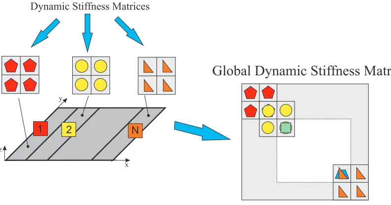
2.4. Assembly procedure, boundary conditions and similarities with FEM

Once the DS matrix of a laminate element has been developed, it can be rotated and/or offset if

required and thus can be assembled to form the global DS matrix of the final structure. The assembly

procedure is schematically shown in Fig. 2 which is similar to that of FEM. Although like the FEM, a

mesh is required in the DSM, it should be noted that the latter is mesh independent in the sense that

additional elements are required only when there is a change in the geometry of the structure. A single

DS laminate element is enough to compute any number of its natural frequencies to any desired accuracy,

which, of course, is impossible in the FEM. However, for the type of structures under consideration DS

plate elements do not have point nodes, but have line nodes instead. In this particular case, no change in

geometry along the longitudinal direction is admitted. This is in addition to the assumed simple support

boundary conditions on two opposite sides, inherent in DSM for plate elements at present. The other

two sides of the plate can have any boundary conditions. The application of the boundary conditions

of the global dynamic stiffness matrix involves the use of the so-called penalty method. This consists

of adding a large stiffness to the appropriate leading diagonal term which corresponds to the degree of

freedom of the node that needs to be suppressed. It is thus possible to apply free (F), simple support (S)

and clamped (C) boundary conditions on the structure by penalizing the appropriate degrees of freedom.

(19)

clamped boundary condition U, V, W, Φy, Φx, W, x will have to be penalized. Of course for the

free-edge boundary condition no penalty will be applied. Because of the similarities between DSM and FEM,

DS elements can be implemented in FEM codes and thus the accuracy of results can be enhanced very

considerably.

2.5. Application of the Wittrick-Williams Algorithm

In order to compute the natural frequencies of a structure by using the DSM, an efficient way to solve

the eigenvalue-problem is to apply the Wittrick-Williams algorithm [3] which has featured in literally

hundreds of papers. For the sake of completeness the procedure is briefly summarized as follows.

First the global dynamic stiffness matrix of the final structureK∗ _{is computed for an arbitrarily chosen}

trial frequency ω∗_{. Next, by applying the usual form of Gauss elimination the global stiffness matrix, is}

transformed into its upper triangularK∗△ _{form. The number of negative terms on the leading diagonal}

of K∗△ _{is now defined as the sign count}_s₍_K∗_{) which forms the fundamental basis of the algorithm. In}

its simplest form, the algorithm states that j, the number of natural frequencies (ω) of a structures that

lie below an arbitrarily chosen trial frequency (ω∗_{) is given by:}

j=j0+s(K∗) (41)

where j0 is the number of natural frequencies of all single elements within the structure which are still

lower than the trial frequency (ω∗_{) when their nodes are fully clamped. It is necessary to account for this}

clamped-clamped frequencies because exact free vibration analysis using DSM allows an infinity number

of natural frequencies to be accounted for when all the nodes of the structures are fully clamped, i.e.

in the overall formulation K δ = 0, these natural frequencies correspond to δ = 0 modes. Thus j0 is

an integral part of the algorithm and not really a peripheral issue. However, unless exceptionally high

frequencies are needed,j0is usually zero and the dominant term of the algorithm is the sign-counts(K∗),

of Eq. (41). One way of avoiding the computation ofj0 is to split the structure into sufficient number of

elements so that the clamped-clamped natural frequencies of an individual element in the structure are

never exceeded. Once s(K∗_{) and}_j₀_{of Eq. (41) are known, any suitable method, for example, bi-section}

technique, can be devised to bracket any natural frequency within any desired accuracy. The mode shapes

are routinely computed by using standard eigenvector recovery procedure in which the global dynamic

stiffness matrix is computed at the natural frequency and the force vector is set to zero whilst deleting

one row of the DS matrix and giving one of the nodal displacement component an arbitrarily chosen

value and then determining the rest of the displacements in terms of the chosen one.

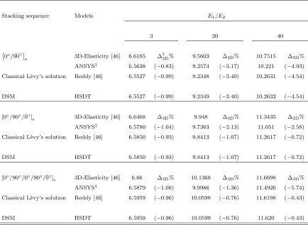
3. Results ans Discussion

The first set of results was obtained to validate the dynamic stiffness theory using HSDT presented

in this paper. For the fundamental natural frequency, Table 1 shows representative results in

non-dimensional form for a cross-ply composite square plate simply supported on all edges using the present

theory along side the published results from literature. Of particular significance, is the inclusion of

(20)

results obtained by the present theory. Note that the ANSYS results were obtained by using SHELL181

element. Results in Table 1 cover a broad range of laminate lay-ups and stacking sequences. It is evident

that the DS theory using HSDT predicts natural frequencies of composite plate in an accurate manner.

The maximum error incurred when compared to 3D elasticity solution is 4.54% for an artificially large

value of the orthotropic ratio E1/E2 = 40. For realistic orthotropic ratios, the error is expected to be

much less. (Note that for carbon-epoxy and glass-epoxy composite structures the ratioE1/E2 is around

10.) The next set of results was obtained to examine the effects of the thickness to length ratio and

the orthotropic ratio on the first four natural frequencies of the square plate, simply supported on all

edges, but with stacking sequence [0◦_/₉₀◦_/₀◦_/₉₀◦_/¯₀◦_]

s. The results using the current DSM based on

HSDT are shown in Table 2 together with the ones obtained by using the DSM program (based on

FSDT) developed by Boscolo and Banerjee [22, 23]. Some interesting observations can be made from

these results. Clearly, the difference in natural frequencies when using the more accurate HSDT and

as opposed to relatively less accurate FSDT, increases when the plate becomes progressively thicker, as

expected. One of the anomalies in using FSDT arises from the difficulty to select the shear corrector

factor (χ), which is generally introduced on an ad-hoc basis in an attempt to account for the correct

shear stress distribution which in reality is not uniform through the cross section. Strictly speaking, the

FSDT can never achieve zero shear stress distribution at the free boundaries. Thus there is an element

of uncertainty in choosing the shear corrector factor and different authors have used different values (see

Mindlin [44] , Reissner [45]). The problem of choosing the shear corrector factor is even more troublesome

for composites. However, this factor is taken to be 5/6 (see [45]) in the FSDT results shown in Table 2.

By contrast the HSDT results based on refined displacement field do not rely on such fictitious (and quite

often arbitrarily chosen) shear correction factor because the HSDT intrinsically account for the parabolic

shear stresses distribution. To confirm the predictable accuracy of the current method, 3D elasticity

solution has been used for comparison purposes. Both the influence of the thickness-to-length ratio and

the orthotropic ratio on results are also shown in Table 2. The next set of results are focused on the

effect of boundary conditions. For two representative values of thickness ratio (b/h), the results in Table

3 show the effects of the boundary conditions on the first four natural frequencies of the above plate.

It should be noted that FSDT results are also included in the table. Clearly, when the plate is simply

supported on to opposite sides and clamped on the other two sides, the natural frequencies assume higher

values as expected. For this case, the maximum error encountered is in the third natural frequency when

using FSDT instead of the more accurate HSDT. The absolute values of these errors are around 7.5%

and 4.2% when the thickness ratios are 5 and 10 respectively, as can be seen in Table 3. It also evident

from the results that on occasions, the FSDT results are lower than the HSDT ones. The reason for this

can be attributed to the fact that the choice of the shear correction factor (which is non-existent and

unnecessary in HSDT), influences the FSDT results in some unpredictable way. Such discrepancies are

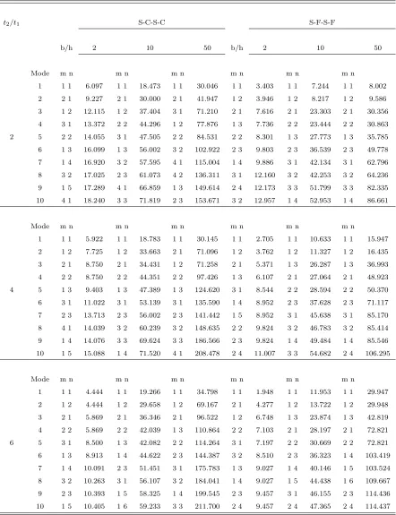
not uncommon and can be found in the literature. In order to demonstrate the applicability of the theory

to an assembly of composite plates, a stepped panel which is schematically shown in Fig. 3 has also been

analysed. As in previous cases, the results were obtained in non-dimensional form and with particular

(21)

representative from a practical standpoint. The results where obtained for different boundary condition,

and for a wide range of thickness ratios between the stiffened plate and parent plate (t2/t1) ranging from

2 to 6. The first ten natural frequencies using the present theory with S-C-S-C and S-F-S-F boundary

conditions, are shown in Table 4 for different values ofb/h. The results shown are exact and cannot be

found in the existing literature, neither can they be obtained in an exact sense using other methods. The

following comments about these results are relevant. Understandably, the natural frequencies are higher

for S-C-S-C boundary conditions compared to S-F-S-F ones, as expected, but more importantly, for thick

plates, e.g. b/h= 2, increasingt2/t1, decreases all the natural frequencies significantly. By contrast, for

relatively thin plates with b/h= 10 the natural frequencies increase with increasing t2/t1 ratio for this

particular problem. The reason for this can be attributed to the fact that for higherb/h ratio the effect

of mass of the stiffened plate appears to be more pronounced than its stiffness, yielding lower natural

frequencies as a consequence. The final set of results was obtained to demonstrate the mode shapes of the

composite plate and the stepped panel using HSDT based DSM. In Figs. 4 to 6, a direct comparison of

the first, fifth and ninth modes between the simple cross-ply laminated composite plate and the stepped

panel has been made for the boundary conditions S-C-S-C, when the step ratio t2/t1 = 2, whilst the

overall dimensions for the two configurations are kept the same. These figures reveal some interesting

features. For the fundamental mode, see Fig. 4, there is hardly any difference in the natural frequency

and mode shape between the simple plate and stepped panel. This is in sharp contrast to the fifth and

ninth modes shown in Figs. 5 and 6 respectively, where some differences in the natural frequencies and

mode shapes are prevalent. It is clear from these two figures that significant alteration in the mode

shapes is possible when required as a result of using stepped panel. The corresponding results for

S-F-S-F boundary condition are shown in Figs. 7, 8 and 9. Figure 7 shows that the fundamental natural

frequency changes significantly, but the mode shape follows more or less the same pattern. The sixth and

ninth modes shown in Figs. 8 and 9, fortuitously reveal the same picture as the fundamental one shown

in Fig. 7. It is interesting to note that for S-C-S-C and S-F-S-F boundary conditions, results and trends

are markedly different. These observations are important when solving frequency attenuation problems

to avoid certain undesirable natural frequencies and mode shapes of complex composite structures.

4. Concluding Remarks

An exact dynamic stiffness theory for composite plate elements using higher order shear deformation

theory is developed for the first time in this paper using Hamiltonian mechanics and symbolic algebra.

The theory is implemented in a computer program to carry out free vibration analysis of composite

structures modelled as plate assemblies. The proposed theory is a significant refinement over recently

developed dynamic stiffness method using classical and first order shear deformation plate theories. The

developed DSM model is particularly useful when analyzing thick composite plates with moderate to high

orthotropic ratios for which the FEM may become unreliable, particularly at high frequencies. A detailed

parametric study has been carried out by varying significant plate parameters and boundary conditions.

The results have been critically examined and the theory has been assessed using existing theories and

(22)

been analyzed for its dynamic behavior. Based on the computed results the following comments can be

made:

• The proposed exact dynamic stiffness composite plate element based on HSDT is shown to be more accurate in terms of results and computational efficiency when compared with FEM in free vibration

analysis of composite plate assemblies.

• The theory provides a significant refinement over FSDT element, particularly when thick plates with high orthotropic ratios are analyzed.

• The boundary conditions do not seem to affect the error incurred using FSDT as opposed to more accurate HSDT.

• The dynamic behavior of stepped composite plates are very different from those of simple com-posite plates depending on the boundary conditions, but significant alteration in mode shapes is possible

by using stepped panels. This could be useful in solving frequency attenuation problems.

References

[1] J. R. Banerjee, Dynamic stiffness formulation for structural elements: A general approach,

Comput-ers & Structures 63 (1) (1997) 101–103.

[2] O. C. Zienkiewicz, The Finite Element Method in Engineering Science, 1st Edition, McGraw Hill,

London, England, 1971.

[3] W. H. Wittrick, F. W. Williams, A general algorithm for computing natural frequencies of elastic

structures, Quarterly Journal of Mechanics and Applied Mathematics 24 (3) (1970) 263–284.

[4] M. S. Anderson, F. W. Williams, J. R. Banerjee, B. J. During, C. L. Herstrom, D. Kennedy, D. B.

Warnaar, User manual for BUNVIS-RG: An exact buckling and vibration program for lattice

struc-tures with repetitive geometry and substructuring option, NASA Technical Memorandum 87669,

1986.

[5] W. H. Wittrick, F. W. Williams, Buckling and vibration of anisotropic or isotropic plate assemblies

under combined loadings, International Journal of Mechanical Sciences 16 (4) (1974) 209–239.

[6] F. W. Williams, Computation of natural frequencies and initial buckling stresses of prismatic plate

assemblies, Journal of Sound and Vibration 21 (1972) 87–106.

[7] R. Plank, W. H. Wittrick, Buckling under combined loadings of thin flat-walled structures by a

complex finite-strip method, International Journal of Numerical Methods in Engineering 8 (1974)

(23)

[8] F. W. Williams, M. S. Anderson, Incorporation of Lagrange multipliers into an algorithm for finding

exact natural frequencies or critical buckling loads, International Journal of Mechanical Sciences

25 (8) (1983) 579–584.

[9] M. S. Anderson, F. W. Williams, C. J. Wright, Buckling and vibration of any prismatic assembly

of shear and compression loaded anisotropic plates with an arbitrary supporting structures,

Inter-national Journal of Mechanical Sciences 25 (8) (1983) 585–596.

[10] D. Kennedy, F. W. Williams, Vibration and buckling of anisotropic plate assemblies with winkler

foundations, Journal of Sound and Vibration 138 (3) (1990) 501–510.

[11] F. W. Williams, D. Kennedy, M. S. Anderson, Analysis features of VICONOPT, an exact

buck-ling and vibration program for prismatic assemblies of anisotropic plates, Proceeding of the 31st

AIAA/ASME/ASCE/AHS/ASC Structures, Structural Dynamics and Materials Conference, Long

Beach, California AIAA Paper 90-0970 (1990) 920–990.

[12] R. Butler, F. W. Williams, Optimum design features of viconopt, an exact buckling and

vibration program for prismatic assemblies of anisotropic plates, Proceeding of the 31st

AIAA/ASME/ASCE/AHS/ASC Structures, Structural Dynamics and Materials Conference, Long

Beach, California AIAA Paper 90-1068 (1990) 1289–1299.

[13] M. S. Anderson, D. Kennedy, Inclusion of transverse shear deformation in the exact

buckling and vibration analysis of composite plate assemblies, Proceeding of the 32nd

AIAA/ASME/ASCE/AHS/ASC Structures, Structural Dynamics and Materials Conference,

Dal-las, Texas, April 13-15 1992 AIAA Paper 92-2287.

[14] D. M. McGowan, Development of curve-plate elements for the exact buckling analysis of

compos-ite plate assemblies including transverse-shear effects, NASA/TM-1999-209512, Langley Research

Center, Hampton, Virginia, USA, 1999.

[15] J. R. Banerjee, Free vibration analysis of a twisted beam using the dynamic stiffness method,

Inter-national Journal of Solids and Structures 38 (38-39) (2001) 6703–6722.

[16] J. R. Banerjee, Free vibration of sandwich beams using the dynamic stiffness method, Computers

and Structures 81 (18-19) (2003) 1915–1922.

[17] J. R. Banerjee, Development of an exact dynamic stiffness matrix for free vibration analysis of a

twisted timoshenko beam, Journal of Sound and Vibration 270 (1-2) (2004) 379–401.

[18] J. R. Banerjee, H. Su, D. R. Jackson, Free vibration of rotating tapered beams using the dynamic

stiffness method, Journal of Sound and Vibration 298 (4-5) (2006) 1034–1054.

[19] J. R. Banerjee, C. W. Cheung, R. Morishima, M. Perera, J. Njuguna, Free vibration of a

three-layered sandwich beam using the dynamic stiffness method and experiment, International Journal

(24)

[20] M. Boscolo, J. R. Banerjee, Dynamic stiffness elements and their applications for plates using first

order shear deformation theory, Computers & Structures 89 (2011) 395–410.

[21] M. Boscolo, J. R. Banerjee, Dynamic stiffness method for exact in-plane free vibration analysis of

plates and plate assemblies, Journal of Sound and Vibrations 330 (12) (2011) 2928–2936.

[22] M. Boscolo, J. R. Banerjee, Dynamic stiffness formulation for composite Mindlin plates for exact

modal analysis of structures. part I: Theory, Computers & Structures 96-97 (2012) 61–73.

[23] M. Boscolo, J. R. Banerjee, Dynamic stiffness formulation for composite Mindlin plates for exact

modal analysis of structures. part II: Results and applications, Computers & Structures 96-97 (2012)

74–83.

[24] J. Reddy, A simple higher order theory for laminated plates., Journal of Applied Mechanics 51 (1984)

745–752.

[25] J. Reddy, D. Phan, Stability and vibration of isotropic , orthotropic and laminate plates according

to a higher-order shear deformation theory., Journal of Sound and Vibration 98 (2) (1985) 157–170.

[26] J. Reddy, T. Kuppusamy, Natural vibration of laminated anisotropic plates., Journal of Sound and

Vibration 94 (1) (1984) 63–69.

[27] B. Vlasov, On the equations of bending of plates, Dokla Ak Nauk Azerbeijanskoi SSR [in Russian]

3 (1957) 955–959.

[28] Jemielita, Technical theory of plates with moderate thickness., Rozprawy Inz [in Polish] 23 (1975)

483–499.

[29] Jemielita, On kinematical assumptions of refined theories of plates., Journal of Applied Mechanics

57 (1990) 1088–1091.

[30] E. Carrera, F. A. Fazzolari, L. Demasi, Vibration analysis of anisotropic simply supported plates

by using variable kinematic and Rayleigh-Ritz method, Journal of Vibration and Acoustics 133 (6)

(2011) 061017–1/061017–16.

[31] F. A. Fazzolari, E. Carrera, Advanced variable kinematics Ritz and Galerkin formulation for accurate

buckling and vibration analysis of laminated composite plates, Composite Structures 94 (1) (2011)

50–67.

[32] F. A. Fazzolari, E. Carrera, Thermo-mechanical buckling analysis of anisotropic multilayered

com-posite and sandwich plates by using refined variable-kinematics theories, Submitted for publication,

2012.

[33] E. Carrera, M. Petrolo, On the effectiveness of higher-order terms in refined beam theories, Journal

of Applied Mechanics 78 (2011) 021013–1021013–17.

(25)

[35] F. A. Fazzolari, Fully coupled thermo-mechanical effect in free vibration analysis of anisotropic

multilayered plates by combining hierarchical plates models and a trigonometric Ritz formulation,

Mechanics of Nano, Micro and Macro Composite Structures, Politecnico di Torino 18-20 June, 2012.

[36] E. Carrera, M. Boscolo, Classical and mixed finite elements for static and dynamic analysis of

piezoelectric plates, International journal for numerical methods in engineering 70 (2007) 1135–1181.

[37] E. Carrera, M. Boscolo, A. Robaldo, Hierarchic multilayered plate elements for coupled multifield

problems of piezoelectric adaptive structures: Formulation and numerical assessment, Archives of

computational methods in engineering 14 (2007) 383–430.

[38] E. Carrera, On the use of transverse shear stress homogeneous and non-homogeneous conditions in

third-order orthotropic plate theory, Composite Structures 77 (2007) 341–352.

[39] J. N. Reddy, Mechanics of Laminated Composite Plates and Shells. Theory and Analysis, 2nd

Edi-tion, CRC Press, 2004.

[40] Y. F. Xing, B. Liu, Exact solutions for the free in-plane vibrations of rectangular plates, International

Journal of Mechanical Sciences 51 (3) (2009) 246–255.

[41] C. I. Park, Frequency equation for the in-plane vibration of a clamped circular plate, Journal of

Sound and Vibration 313 (1-2) (2008) 325–333.

[42] D. Gorman, Exact solutions for the free in-plane vibration of rectangular plates with two opposite

edges simply supported, Journal of Sound and Vibration 294 (1-2) (2006) 131–161.

[43] Y. F. Xing, B. Liu, New exact solutions for free vibrations of thin orthotropic rectangular plates,

Composite Structures 89 (4) (2009) 567–574.

[44] R. D. Mindlin, Influence of rotary inertia and shear on flexural motions of isotropic elastic plates.,

Journal of Applied Mechanics 18 (10) (1951) 1031–1036.

[45] E. Reissner, On the theory of bending of elastic plates, Journal of Mathematical Physics 23 (4)

(1944) 184–191.

[46] T. Kant, K. Swaminathan, Free vibration of isotropic, orthotropic, and multilayer plates based on

(26)

[image:26.595.82.516.150.467.2]

Tables

Table 1: Dimensionless fundamental natural frequency parameter ˆω = ω b h

q _ρ

E2, for a cross-ply square composite plate simply supported at all edges witha/h= 5,E1/E2= open,G12/E2=G13/E2= 0.6,G23/E2= 0.5,ν12=ν13= 0.25.

Stacking sequence Models E1/E2

3 20 40

0◦_/₉₀_¯◦

s 3D-Elasticity [46] 6.6185 ∆ †

3D% 9.5603 ∆3D% 10.7515 ∆3D%

ANSYS‡ ₆_.₅₆₃₈ ₍₋₀_.₈₃₎ ₉_.₂₅₇₄ ₍₋₃_.₁₇₎ ₁₀_.₂₂₁ ₍₋₄_.₉₃₎

Classical L`evy’s solution Reddy [46] 6.5527 (−0.99) 9.2348 (−3.40) 10.2631 (−4.54) DSM HSDT 6.5527 (−0.99) 9.2349 (−3.40) 10.2632 (−4.54) [0◦_/₉₀◦_/_¯₀◦_]

s 3D-Elasticity [46] 6.6468 ∆3D% 9.948 ∆3D% 11.3435 ∆3D%

ANSYS‡ ₆_.₅₇₈₀ ₍₋₁_.₀₄₎ ₉_.₇₃₆₃ ₍₋₂_.₁₃₎ ₁₁_.₀₅₁ ₍₋₂_.₅₈₎

Classical L`evy’s solution Reddy [46] 6.5850 (−0.93) 9.8413 (−1.07) 11.2617 (−0.72) DSM HSDT 6.5850 (−0.93) 9.8413 (−1.07) 11.2617 (−0.72) [0◦_/₉₀◦_/₀◦_/₉₀◦_/_¯₀◦_]

s 3D-Elasticity [46] 6.66 ∆3D% 10.1368 ∆3D% 11.6698 ∆3D%

ANSYS‡ ₆_.₅₈₇₉ ₍₋₁_.₀₈₎ ₉_.₉₉₈₆ ₍₋₁_.₃₆₎ ₁₁_.₄₉₂₆ ₍₋₅_.₇₄₎