High-mass Starless Clumps in the Inner Galactic Plane: The Sample and Dust Properties
Jinghua Yuan (袁敬华)1,10,
Yuefang Wu(吴月芳)2, Simon P. Ellingsen3, Neal J. Evans II4,5, Christian Henkel6,7,
Ke Wang(王科)8, Hong-Li Liu(刘洪礼)1, Tie Liu(刘铁)5, Jin-Zeng Li(李金增)1, and Annie Zavagno9
1
National Astronomical Observatories, Chinese Academy of Sciences, 20A Datun Road, Chaoyang District, Beijing 100012, China;[email protected]
2
Department of Astronomy, Peking University, 100871 Beijing, China 3
School of Physical Sciences, University of Tasmania, Hobart, Tasmania, Australia
4Department of Astronomy, The University of Texas at Austin, 2515 Speedway, Stop C1400, Austin, TX 78712-1205, USA 5
Korea Astronomy and Space Science Institute 776, Daedeokdae-ro, Yuseong-gu, Daejeon 34055, Korea 6
Max-Planck-Institut für Radioastronomie, Auf dem Hügel 69, D-53121 Bonn, Germany 7
Astron. Dept., King Abdulaziz University, P.O. Box 80203, Jeddah 21589, Saudi Arabia 8
European Southern Observatory, Karl-Schwarzschild-Str. 2, D-85748 Garching bei München, Germany 9
Aix Marseille Universit, CNRS, LAM(Laboratoire d’Astrophysique de Marseille)UMR 7326, F-13388, Marseille, France
Received 2016 December 23; revised 2017 March 30; accepted 2017 May 5; published 2017 July 20
Abstract
We report a sample of 463 high-mass starless clump (HMSC) candidates within - < <60 l 60 and b
1 1
- < < . This sample has been singled out from 10,861 ATLASGAL clumps. None of these sources are associated with any known star-forming activities collected in SIMBAD and young stellar objects identified using color-based criteria. We also make sure that the HMSC candidates have neither point sources at 24 and 70μmnor strong extended emission at 24μm. Most of the identified HMSCs are infrared dark, and some are even dark at 70μm. Their distribution shows crowding in Galactic spiral arms and toward the Galactic center and some well-known star-forming complexes. Many HMSCs are associated with large-scalefilaments. Some basic parameters were attained from column density and dust temperature maps constructed viafitting far-infrared and submillimeter continuum data to modified blackbodies. The HMSC candidates have sizes, masses, and densities similar to clumps associated with Class II methanol masers and HIIregions, suggesting that they will evolve into star-forming clumps. More than 90% of the HMSC candidates have densities above some proposed thresholds for forming high-mass stars. With dust temperatures and luminosity-to-high-mass ratios significantly lower than that for star-forming sources, the HMSC candidates are externally heated and genuinely at very early stages of high-mass star formation. Twenty sources with equivalent radiireq<0.15pc and mass surface densitiesS > 0.08g cm−2could be possible
high-mass starless cores. Further investigations toward these HMSCs would undoubtedly shed light on comprehensively understanding the birth of high-mass stars.
Key words:infrared: ISM– ISM: clouds–stars: formation– stars: massive– submillimeter: ISM Supporting material:figure sets, machine-readable tables
1. Introduction
High-mass stars, through mechanical and radiative input, play crucial roles in the structural formation and evolution in galaxies. They are also the primary contributor of chemical enrichment in space. However, the forming process of high-mass stars still remains a mystery (Tan et al.2014).
The turbulent core and competitive accretion models have been proposed as alternative scenarios for the formation of massive stars(Bonnell et al.2001; McKee & Tan2003). In the turbulent core model, thefinal stellar mass is pre-assembled in the collapsing core, so this model requires the existence of high-mass starless cores. In contrast, the competitive accretion model predicts that high-mass stars begin as clusters of small cores with masses peaked around the Jeans mass of the clump and there is no connection between the mass of its birth core and the final stellar mass. Discriminating between these two models requires identification of the youngest high-mass star formation regions to enable investigation of the initial conditions.
Starless clumps are the objects that fragment into dense starless cores (r<0.15 pc), which subsequently contract to form individual or bound systems of protostars (Tan et al. 2014). Despite many searches, there are only a few candidate high-mass starless cores known to date (e.g., Wang et al. 2011, 2014; Tan et al. 2013; Cyganowski et al. 2014; Kong et al. 2017). Recently, one of the most promising candidates, G028.37+00.07(C1), was removed from the list because ALMA and NOEMA observations reveal protostellar outflows driven by the core(Feng et al.2016; Tan et al.2016). Although a high-resolution, deep spectral imaging survey is the ultimate way to verify the starless nature, such a survey must start from a systematic sample. More candidate cores embedded within high-mass starless clumps (HMSCs) are essentially required so that some statistical understanding can be achieved. How dense clumps fragment is another key question that must be answered to understand high-mass star formation, especially in the competitive accretion scenario. Although fragments with super-Jeans masses have been revealed in some infrared dark clouds (IRDCs) with ongoing star-forming activity (e.g., Wang et al. 2011, 2014; Beuther et al.2013,2015; Zhang et al.2015), whether the HMSCs can fragment into Jeans-mass cores is still a key open question. Therefore, identification and investigations of HMSCs are
© 2017. The American Astronomical Society. All rights reserved.
10
FITS images for the far-IR to submillimeter data, H2column density, and
essential to understanding the formation of high-mass stars and clusters.
Recent Galactic plane surveys of dust continuum emission have revealed numerous dense structures at a wide range of evolutionary stages, including the starless phases. The APEX Telescope Large Area Survey of the Galaxy (ATLASGAL; Schuller et al. 2009), the Bolocam Galactic Plane Survey (BGPS; Aguirre et al. 2011; Dunham et al. 2011), and the Herschel Infrared Galactic Plane Survey (Hi-GAL; Molinari et al. 2010) have revealed extended dust emission at far-Infrared (IR)to submillimeter, while surveys at near- to mid-IR, such as the Galactic Legacy Infrared Mid-Plane Survey Extraordinaire survey (GLIMPSE; Benjamin et al. 2003; Churchwell et al. 2009)and the Galactic Plane Survey using the MIPS(MIPGSGAL), reveal emissions from warm/hot dust and young stars. The combination of these surveys provides us an unprecedented opportunity to identify a large sample of candidate starless clumps.
Recently, Tackenberg et al. (2012), Traficante et al. (2015), and Svoboda et al. (2016)have identified 210, 667, and 2223 starless clump candidates in the longitude ranges10 < <l 20,
l
15 < <55, and10 < <l 65, respectively. These
endea-vors have revealed some properties of early stages of star formation. However, these samples use criteria that do not allow them to reliably discriminate between low-mass and high-mass clumps and in some cases may have misidentified star-forming objects(see Section3.2). Also, the covered longitude ranges are limited.
In this work, we identify a sample of HMSCs with better coverage of Galactic longitude (- < <60 l 60) based on multiwavelength data from the GLIMPSE, MIPSGAL, Hi-GAL, and ATLASGAL surveys. The data used in this work are described in Section 2. The identification procedure is described in Section 3. In Section 4, we outline distance estimation and spatial distributions. Based on continuum data from 160 to 870μm, some dust parameters are derived in Section 5. More in-depth discussions and a summary of the findings are given in Sections6and 7.
2. Data
This work is based on data from several Galactic plane surveys covering wavelengths from mid-IR to submillimeter. The sample of dense clumps from the ATLASGAL survey11 (Schuller et al.2009)provides the basis for our investigation. The ATLASGAL survey mapped 420 square degrees of the Galactic plane between - < < + ,80 l 60 using the LABOCA camera on the APEX telescope at 870μmwith a 19 2 angular resolution. The astrometry of the data set and the derived source positions have been assumed to be the same as the pointing accuracy of the telescope, which is ~ 2 –3
(Contreras et al.2013). The absoluteflux density uncertainty is estimated to be better than 15% (Schuller et al. 2009). Structures larger than 2 5 have been filtered out during the reduction of the raw data because the emission from the atmosphere mimics that from extended astronomical objects. Thefinal maps, gridded into3 ´ 3 tiles with a pixel size of 6″, are available from the project site.12The average noise in
the maps was determined from the∣ ∣b < 1 portions of the maps to be about 70 mJy beam−1. On the basis of these maps, two source catalogs have been produced using the Gaussclump (Csengeri et al. 2014) and SExtractor (Contreras et al. 2013; Urquhart et al. 2014a) algorithms. The Gaussclump source catalog with 10,861 sources has been optimized for small-scale embedded structures (i.e., nearby cores and distant clumps), with background emission from molecular clouds removed (Csengeri et al.2014). On the other hand, the 10,163 compact sources extracted using the SExtractor algorithm are represen-tatives of larger-scale clump or cloud structures. In this work, we have used the Gaussclump source catalog of Csengeri et al. (2014)as the parent sample to identify starless clumps.
Point-source catalogs from GLIMPSE and MIPSGAL surveys have been used to identify possible young stellar object(YSO)candidates associated with ATLASGAL clumps. Using the IRAC instrument on board the Spitzer Space Telescope(Werner et al.2004), the GLIMPSE project surveyed the inner 130 of the Galactic plane at 3.6, 4.5, 5.8, and 8.0μmwith 5s sensitivities of 0.2, 0.2, 0.4, and 0.4 mJy, respectively. In addition to the images, the GLIMPSE survey performed point-source photometry, which, in combination with the Two Micron All Sky Survey point-source catalog (Skrutskie et al. 2006), provides photometric data of point sources in seven infrared bands. The MIPSGAL survey used the Multiband Infrared Photometer on Spitzer (Carey et al.2009)to map an area comparable to GLIMPSE at longer infrared wavelengths. Version 3.0 of the MIPSGAL data includes mosaics from only the 24μmband, with a sky coverage of ∣ ∣b < 1 for - < <68 l 69 and ∣ ∣b < 3 for
l
8 9
- < < . The angular resolution and 5s sensitivity at 24μmare 6″and 1.7 mJy, respectively. The images and point-source catalogs of both GLIMPSE and MIPSGAL are available at the InfraRed Science Archive(IRSA).13
Far-IR data from the Hi-GAL survey have been used to further constrain the starless clump candidates and investigate their dust properties. Hi-GAL is a key project of theHerschel Space Observatory, which mapped the entire Galactic plane with nominal∣ ∣b 1 (following the Galactic warp). The Hi-GAL data were taken in fast scan mode (60″ s−1) using the PACS (70 and 160μm) and SPIRE (250, 350, and 500μm) instruments in the parallel mode. The maps have been reduced with the ROMAGAL pipeline (Traficante et al. 2011), an enhanced version of the standardHerschelpipeline specifically designed for Hi-GAL. The effective angular resolutions are
10. 2 ,13. 5 ,18. 1 ,24. 9 , and36. 4 at 70, 160, 250, 350, and 500μm, respectively.
3. The High-mass Starless Clumps Catalog
3.1. Source Identification
We have combined information from the GLIMPSE, MIPSGAL, Hi-GAL, and ATLASGAL surveys to identify starless clumps. Reliable identification requires the combina-tion of data from all four surveys, and so only ATLASGAL clumps in the inner Galactic plane(∣ ∣l <60and∣ ∣b < 1 )that meet this criterion have been considered. To identify candidate HMSCs, we have applied the procedure outlined in Figure1to the ATLASGAL sources in the region of interest.
11
The ATLASGAL project is a collaboration between the Max-Planck-Gesellschaft, the European Southern Observatory(ESO), and the Universidad de Chile. It includes projects E-181.C-0885, E-078.F-9040(A), M-079.C-9501
(A), and M-081.C-9501(A)plus Chilean data. 12
As we mainly aim tofind the birth sites of high-mass stars, a threshold for the peak intensity at 870μmis essential to identify high-mass clumps. Here, we followed Tackenberg et al.(2012) and select only objects with peak intensities higher than 0.5 Jy beam−1. Assuming a dust opacity ofk870=1.65cm2g−1
and a dust temperature of 15 K, this threshold corresponds to a column density of2.2´1022cm−2. Although smaller than the theoretical threshold value proposed by Krumholz & McKee (2008), which is about 1 g cm−2or 2.15´1023cm−2, we consider this to be a reasonable value considering the beam dilution that will occur owing to the intermediate angular resolution of theAPEXobservations. The effects of distance and telescope resolution on measurements of peak column density have been studied by Vasyunina et al.(2009)under an assumed r-1 density distribution. The peak column density at a spatial resolution of 0.01 pc can be diluted by a factor of tens at∼3 kpc if it is observed using a single-dish telescope with an angular resolution of 11″–24″(Vasyunina et al.2009). Even assuming a crude correction factor of 10, clumps with peak intensities higher than 0.5 Jy beam−1 likely contain unresolved subregions with column densities higher than2.15´1023cm−2
.
These first two criteria reduce the number of ATLASGAL sources under consideration by more than a factor of 2, with 5279 clumps remaining under consideration. For these clumps we have used the SIMBAD database to search for a wide range of associated star-formation-related phenomena. We queried the SIMBAD database for star-formation-associated objects within a circle defined by the major axis of the Gaussian ellipse given in Csengeri et al.(2014). If an object belonging to any of the 18 categories listed in Table1was found within this region, we consider the ATLASGAL source a likely star-forming
region and exclude it from our sample. This query to SIMBAD also successfully removes clumps associated with star-forming phenomena investigated in some large surveys, such as the 6.7 GHz methanol masers (Breen et al. 2013), the red MSX sources (Lumsden et al. 2013), and HIIregions (Urquhart et al.2013).
We then further identify possible star-forming regions using data from the GLIMPSE point-source catalog and applying the color criteria given in Gutermuth et al.(2009). Any GLIMPSE source with colors that fulfill the criteria below is considered as a YSO candidate, and if any such sources lie within the region of the ATLASGAL clump, it was excluded from our starless clump sample:
3.6 - 4.5 >0.7 and 4.5 - 5.8 >0.7 or
[ ] [ ] [ ] [ ]
3.6 4.5 0.15 and,
3.6 5.8 0.35 and,
4.5 8.0 0.5 and,
3.6 5.8 0.14
0.04
4.5 8.0 0.5 0.5.
1 2 3 2 3 s s s s s
- - >
- - >
- - >
- + ´ - - - + ⎧ ⎨ ⎪ ⎪⎪ ⎩ ⎪ ⎪ ⎪ [ ] [ ] [ ] [ ] [ ] [ ] [ ] [ ] (([ ] [ ] ) )
Here s1=s([3.6]–[4.5]), s2=s([3.6]–[5.8]), and s3=s
4.5 8.0
([ ]–[ ])are combined errors, added in quadrature. In a recent study, Gallaway et al. (2013) show that 17% of methanol masers from the Methanol Multi-Beam(MMB)survey are not associated with emission seen in GLIMPSE, indicating that some very young high-mass stars may be too cold to be detectable in IRAC bands but show weak 24μmemission. Thus, any clump that is associated with a 24μmpoint source probably hosts star-forming activity and should be omitted. By querying the VizieR Service,14 we seized and excluded clumps that are possibly associated with 24μmpoint sources provided in Gutermuth & Heyer (2015). Furthermore, some very faint point sources at 24μmcould have been missed from the catalog of Gutermuth & Heyer(2015), due to bright extended emission contamination. In order to obtain a reliable sample of HMSCs, we also have ignored clumps associated with 24μmextended structures brighter than 103MJy sr−1. This threshold corresponds to about 2.0 mag within an aperture of6. 35 , close to the 90% differential completeness limit(∼1.98 mag)of 24μmpoint sources in bright and structured regions(Gutermuth & Heyer2015).
[image:3.612.48.290.53.359.2]A total of 1215 ATLASGAL compact sources remain after applying these exclusion criteria. These clumps were then subjected to afinal visual inspection to identify(and exclude) any that have very faint 24μmpoint emission missed from the
Figure 1. Flowchart describing the identification procedure of high-mass starless clumps from ATLASGAL compact sources.
Table 1
Star-forming Indicators in SIMBAD
Object Type Object Type
Radio source Young stellar object
Centimetric radio source Young stellar object candidate HII(ionized)region Pre-main-sequence star
Infrared source Pre-main-sequence star candidate
Far-IR source(l30μm) T Tau-type star Near-IR source(l<10μm) T Tau star candidate Herbig–Haro object Herbig Ae/Be star
Outflow Possible Herbig Ae/Be star
Outflow candidate Maser
14
[image:3.612.319.569.74.187.2]Gutermuth & Heyer (2015) catalog, any that are saturated at 24μm, and any that are associated with 70μmpoint-like sources (Molinari et al.2016b).
In the procedures of removing star-forming clumps, some star-forming activities could be in the foreground, leading to underestimating the number of starless clumps. However, the main goal of this work is to identify a more reliable sample of HMSCs, not a complete catalog. The resulting sample contains 463 HMSC candidates, which are listed in Table 2. We find that most of the HMSC candidates are associated with IRDCs; about 49%(229/463)are even dark at 70μm(see Figure2and column (11) of Table 2). Further inspection using far-IR continuum data supports the dense and cold nature of these sources (see Sections5 and6).
3.2. Comparison with Reported Starless Clump Catalogs
There are three previous papers that have searched for starless clumps. Tackenberg et al.(2012)reported a sample of 210 starless clumps in the10 < <l 20 range. Star-forming clumps were ruled out via identifying YSOs from the GLIMPSE catalog based on IR colors and visual analysis of 24μmimages (Tackenberg et al. 2012). Loose criteria for filtering out star-forming clumps led to a greater than 50% misidentification in the Tackenberg et al. (2012) catalog (Svoboda et al. 2016). Among the 210 starless clumps of Tackenberg et al. (2012), only 107 have counterparts in the ATLASGAL GaussClump Catalog(Csengeri et al.2014), and more than 70% (75/107) are possible star-forming clumps if diagnosed using the criteria applied in this work.
In the 15 < <l 55 and ∣ ∣b < 1 area, Traficante et al. (2015) identified 667 starless clumps in IRDCs based on
Hi-GAL data. The Hyper algorithm was used for clump extraction, and counterparts at 70μmwere used for protostellar identification. Spatial cross-matching shows that 175 starless clumps from Traficante et al. (2015)have counterparts in the ATLASGAL catalog, and only 20(~11%)are associated with HMSC candidates identified in this work. The remaining 89% (155/175) possibly can only form low-mass stars or already host star-forming activity. Traficante et al. (2015) suggested that about 26% of their starless clumps have the potential to form high-mass stars. This suggests that about 50% of starless clumps reported in Traficante et al. (2015) may already have started forming stars.
Another catalog of starless clumps has been compiled by Svoboda et al. (2016) based on Bolocam survey data. Star-forming indicators including mid- to far-IR YSOs, masers, and ultracompact HIIregions were considered to rule out clumps with current star formation. Among the 2223 starless clumps in
l
10 < <65from Svoboda et al.(2016), 179 have counter-parts in the ATLASGAL catalog, and 35(20%)are associated with HMSC candidates identified in this work. As noted in Svoboda et al.(2016), about 10% of their starless clumps have the potential to form high-mass stars.
In brief, we may have singled out the by far largest sample of relatively reliable HMSC candidates distributed throughout the whole inner Galactic plane.
4. Distances and Spatial Distribution
4.1. Distance Estimation
[image:4.612.46.569.74.307.2]The distance to a source is a fundamental parameter that is essential to determine its mass and luminosity. The distance to
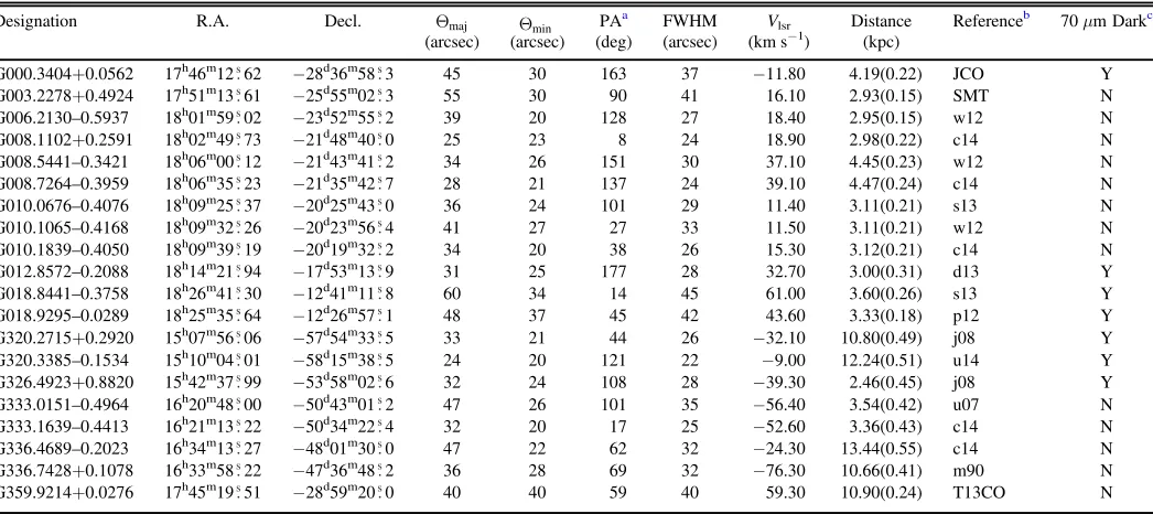
Table 2
Basic Parameters of HMSC Candidates
Designation R.A. Decl. Qmaj Qmin PA
a
FWHM Vlsr Distance Reference
b
70μmDarkc
(arcsec) (arcsec) (deg) (arcsec) (km s−1) (kpc)
G000.3404+0.0562 17h46m12 62 −28d36m58 3 45 30 163 37 −11.80 4.19(0.22) JCO Y
G003.2278+0.4924 17h51m13 61 −25d55m02 3 55 30 90 41 16.10 2.93(0.15) SMT N
G006.2130–0.5937 18h01m59 02 −23d52m55 2 39 20 128 27 18.40 2.95(0.15) w12 N
G008.1102+0.2591 18h02m49 73 −21d48m40 0 25 23 8 24 18.90 2.98(0.22) c14 N
G008.5441–0.3421 18h06m00 12 −21d43m41 2 34 26 151 30 37.10 4.45(0.23) w12 N
G008.7264–0.3959 18h06m35 23 −21d35m42 7 28 21 137 24 39.10 4.47(0.24) c14 N
G010.0676–0.4076 18h09m25 37 −20d25m43 0 36 24 101 29 11.40 3.11(0.21) s13 N
G010.1065–0.4168 18h09m32 26 −20d23m56 4 41 27 27 33 11.50 3.11(0.21) w12 N
G010.1839–0.4050 18h09m39 19 −20d19m32 2 34 20 38 26 15.30 3.12(0.21) c14 N
G012.8572–0.2088 18h14m21 94 −17d53m13 9 31 25 177 28 32.70 3.00(0.31) d13 Y
G018.8441–0.3758 18h26m41 30 −12d41m11 8 60 34 14 45 61.00 3.60(0.26) s13 Y
G018.9295–0.0289 18h25m35 64 −12d26m57 1 48 37 45 42 43.60 3.33(0.18) p12 Y
G320.2715+0.2920 15h07m56 06 −57d54m33 5 33 21 44 26 −32.10 10.80(0.49) j08 Y
G320.3385–0.1534 15h10m04 01 −58d15m38 5 24 20 121 22 −9.00 12.24(0.51) u14 Y
G326.4923+0.8820 15h42m37 99 −53d58m02 6 32 24 108 28 −39.30 2.46(0.45) j08 Y
G333.0151–0.4964 16h20m48 00 −50d43m01 2 47 26 101 35 −56.40 3.54(0.42) u07 N
G333.1639–0.4413 16h21m13 22 −50d34m22 4 32 20 17 25 −52.60 3.36(0.43) c14 N
G336.4689–0.2023 16h34m13 27 −48d01m30 0 47 22 62 32 −24.30 13.44(0.55) c14 N
G336.7428+0.1078 16h33m58 22 −47d36m48 2 36 28 69 32 −76.30 10.66(0.41) m90 N
G359.9214+0.0276 17h45m19 51 −28d59m20 0 40 40 59 40 59.30 10.90(0.24) T13CO N
Notes.
a
Position angle corrected in the FK5 system with respect to the north direction. b
References for systemic velocity.c14: Csengeri et al.2014; d11: Dunham et al.2011; d13: Dempsey et al.2013; j08: Jackson et al.2008; p12: Purcell et al.2012; s13: Shirley et al.2013; u07: Urquhart et al.2007; u14: Urquhart et al.2014b; w12: Wienen et al.2012; m90: MALT90; JCO: CO from the JCMT archive; T13CO:
13COfrom the ThrUMMS survey; SMT: single-point observations using SMT.
c
“Y”indicates that the clump is associated with the extinction feature at 70μm.
the HMSC candidates is not known for most sources, and to address this, we have collected the systemic velocities from the literature for 294 clumps. For a further 20, 63, and 58 sources, velocity measurements have been obtained based on data collected from the MALT90 survey (Jackson et al.2013), the ThrUMMS survey(Barnes et al.2015), and the JCMT archive. Velocities for the remaining 28 sources were determined via single-point observations of 13CO(2 -1) or C18O(2 -1)
using the Submillimeter Telescope(SMT)of the Arizona Radio Observatory. For all of the HMSCs, distance estimates were obtained using a parallax-based distance estimator.15 Lever-aging results of trigonometric parallaxes from the BeSSeL(Bar and Spiral Structure Legacy Survey) and VERA (Japanese VLBI Exploration of Radio Astrometry)projects, the distance estimator can reasonably resolve kinematic distance ambigu-ities based on the Bayesian approach (Reid et al. 2016). The distances calculated using the FORTRAN version of the estimator are given in column(9)of Table2. The 463 HMSCs have distances ranging from 0.3 to 18.3 kpcwith a mean of 7.1 kpcand a median of 6.0 kpc.
The equivalent radius(req)of the ATLASGAL clumps was estimated by multiplying the distance by the deconvolved
equivalent angular radius eq maj min HPBW
2
q = Q Q -q , where
19. 2 HPBW
q = is the ATLASGAL beam. The major and minor
half-intensity axes (Qmaj and Qmaj) were obtained from Csengeri et al.(2014). The resultant equivalent radii are given in column(2)of Table3. The HMSC candidates have a median equivalent radius of 0.65 pc, consistent with that of clumps identified in some IRDCs(∼0.6 pc; Traficante et al.2015)and that of BGPS clumps(∼0.64 pc; Svoboda et al.2016).
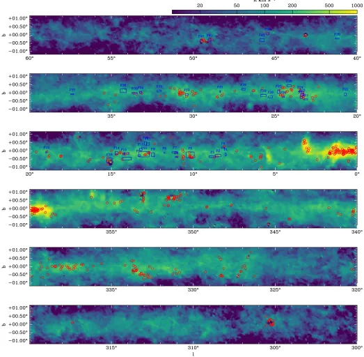
4.2. Spatial Distribution
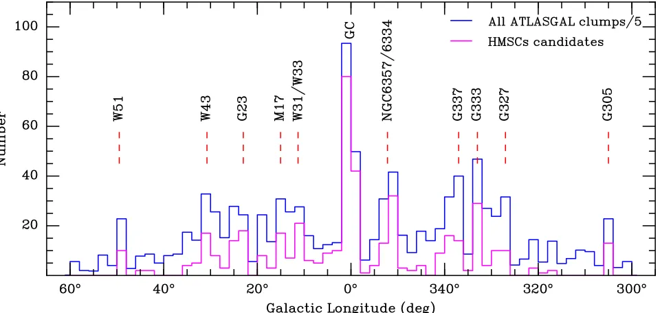
The distributions of the identified HMSC candidates in the inner Galactic plane and as a function of Galactic longitude are shown in Figures 3 and 4, respectively. The distribution of HMSCs in Galactic longitude is very similar to that of the full sample of ATLASGAL clumps. A prominent overdensity can be observed toward the Galactic center region. In addition, there are several well-known star-forming complexes (i.e., W51, W43, G23, M17, W31/W33, NGC 6334/6357, G337, G333, G327, and G305) standing out with significant peaks. Many of the HMSCs are associated with large-scale filaments identified by Wang et al. (2016). In the longitude range 7.5 < <l 60
[image:5.612.46.573.55.380.2]covered by both Wang et al.(2016)and this study, there are 145 HMSCs, 39 of which are located on large-scalefilaments. This implies that about 27% (39/145) of future high-mass star formation would take place in large-scale(>10pc)filamentary structures in the Galactic plane.
Figure 2.Morphology of two example HMSCs in different wavelength bands.(a)Three-color images with emission at 8.0, 4.5, and 3.6μmrendered in red, green, and blue, respectively.(b),(c),(d)show dust continuum emission at 24, 70, and 250μm, respectively. In panel(d), emission at 870μmis presented in red contours with levels of 0.3, 0.4, 0.5, 0.7, 0.9, 1.3, 1.8, 2.5, 4, 7 Jy beam−1. The white plus sign gives the peak position of 870μm, and the white ellipse delineates the source size based on the major and minor half-intensity axes provided in the ATLASGAL catalog.
(The completefigure set(463 images)is available.)
15
To determine the locations of these HMSCs in our Galaxy, we have plotted the sources on a top-down schematic of the Milky Way(see Figure5). Most targets are located in spiral arms in the inner Galaxy with galactocentric distances Rgal<8.34 kpc.
Most sources in the general direction of W51 (l~49) are located in the Carina–Sagittarius arm, with an average distance of about 6 kpc, consistent with that of the W51 complex(Sato et al.2010). Sources toward W43(l~31)and G23(l~23)
mostly reside in the Scutum–Centaurus arm, and some in the near 3 kpc arm. The overdensities atl=10 17– are associated with the W31 and W33 complexes and the well-known star-forming region M17. The sources in this Galactic longitude range are mostly located in the Scutum–Centaurus arm, with some in the Perseus and Norma arms with distances larger than 10 kpc. The peak at l=352 originates from two groups of sources, with the near group associated with the relatively nearby complex of NGC 6334/6357(Russeil et al.2010)located in the Carina–Sagittarius arm and the far group located in the Galactic bar. The peaks toward G327, G333, and G337 are mostly located in the Scutum–Centaurus arm, and some in the Perseus, Norma, and near 3 kpc arms. The sources in the Crux–Scutum arm at this direction have an average distance of about 3.5 kpc, consistent with that of the G333.2–0.4 giant molecular cloud (Simpson et al.2012). Sources atl=305are mostly located at the tangent point of the Crux–Scutum arm.
5. Dust Properties
For all 463 HMSC candidates, there are image data at six far-IR to submillimeter bands covering wavelengths from 70 to 870μmcollected by the Hi-GAL and ATLASGAL surveys, enabling us to obtain some physical parameters. As these sources effectively do not emit at 70μm, we only take emission at 160, 250, 350, 500, and 870μminto account to obtain physical parameters.
5.1. Convolution to a Common Resolution and Foreground/ Background Filtering
In order to be able to estimate physical properties from multiwavelength observations with different angular resolu-tions, we first convolved the images to a common angular resolution of36. 4 , which is essentially the poorest resolution of any of the wavelengths. Theconvolutionpackage ofAstropy (Astropy Collaboration et al.2013)was used with a Gaussian kernel of 36. 4 - q2l, whereqlis the HPBW beam size for a
given Hi-GAL or ATLASGAL band. Then the convolved data from the different bands were regridded to be aligned pixel by pixel with a common pixel size of11. 5 .
[image:6.612.44.568.74.307.2]As our targets are in the Galactic plane, foreground/ back-ground removal is essential to reduce the uncertainties in some of the derived parameters. For the ATLASGAL images, any uniform astronomical signal on spatial scales larger than 2. 5¢ has been filtered out together with atmospheric emission during the data reduction(Schuller et al.2009). Thefiltering of Hi-GAL images was performed using the CUPID-findback algorithm of the Starlink suite.16 The algorithm constructs the background iteratively from the original image. At first, a filtered form of the input data is produced by replacing every input pixel by the minimum of the input values within a rectangular box centered on the pixel. Thisfiltered data are then filtered again, using afilter that replaces every pixel value by the maximum value in a box centered on the pixel. Then each pixel in these filtered data is replaced by the mean value in a box centered on the pixel. The same box size is used for the first three steps. The final background estimate is obtained via some corrections and iterations through comparison with the initial input data. For further details on the algorithm please see the online document for findback.17As a key parameter, thefiltering box was chosen to be
Table 3
Physical Parameters of HMSC Candidates
Designation req Tdust NH2 nH2 Smass Mcl Lcl Lcl Mcl
(pc) (K) (1022cm−2) (104cm−3) (g cm−2) (M) (L) (L
e/Me)
G000.3404+0.0562 0.64 17.08 18.44 3.26 0.40 2.44e+03 4.83e+03 1.98
G003.2278+0.4924 0.51 14.37 3.14 0.61 0.06 2.34e+02 1.88e+02 0.80
G006.2130–0.5937 0.29 15.75 3.49 2.36 0.13 1.67e+02 2.44e+02 1.46
G008.1102+0.2591 0.21 18.41 2.72 5.13 0.21 1.33e+02 4.76e+02 3.58
G008.5441–0.3421 0.49 12.32 4.23 1.25 0.12 4.27e+02 1.41e+02 0.33
G008.7264–0.3959 0.32 12.52 6.88 7.86 0.49 7.54e+02 2.48e+02 0.33
G010.0676–0.4076 0.34 18.78 2.04 1.13 0.07 1.24e+02 5.48e+02 4.43
G010.1065–0.4168 0.41 18.38 2.71 0.82 0.06 1.64e+02 6.05e+02 3.69
G010.1839–0.4050 0.27 22.43 1.77 1.55 0.08 8.55e+01 1.20e+03 13.98
G012.8572–0.2088 0.29 17.35 5.31 3.65 0.21 2.67e+02 6.60e+02 2.47
G018.8441–0.3758 0.71 14.30 4.38 0.58 0.08 6.09e+02 5.12e+02 0.84
G018.9295–0.0289 0.61 18.18 3.22 0.52 0.06 3.36e+02 1.40e+03 4.16
G320.2715+0.2920 0.94 12.15 2.87 0.74 0.13 1.81e+03 5.19e+02 0.29
G320.3385–0.1534 0.63 16.00 4.16 4.82 0.58 3.43e+03 5.52e+03 1.61
G326.4923+0.8820 0.24 13.88 8.22 7.26 0.33 2.85e+02 1.76e+02 0.62
G333.0151–0.4964 0.50 17.60 5.45 1.60 0.16 5.86e+02 1.37e+03 2.34
G333.1639–0.4413 0.27 18.91 6.84 7.31 0.38 4.10e+02 1.69e+03 4.13
G336.4689–0.2023 1.68 14.19 2.25 0.21 0.07 2.85e+03 2.20e+03 0.77
G336.7428+0.1078 1.31 22.16 1.54 0.16 0.04 1.02e+03 1.42e+04 13.86
G359.9214+0.0276 1.85 18.56 6.24 0.32 0.11 5.88e+03 2.09e+04 3.56
(This table is available in its entirety in machine-readable form.)
16
http://starlink.eao.hawaii.edu/starlink/WelcomePage
17
2. 5¢ for consistency with the ATLASGAL data. One drawback of the findback algorithm is that the background can be over-estimated when processing high signal-to-noise data, especially when there are strong emission features significantly smaller than the box size. To mitigate issues with overestimation of the background level, we set the parameter NEWALG to TRUE and iteratively ranfindback. The background image resulting from the previous run was used as the input data for the next iteration. After careful examination of a number of test sources, we found that the resulting background images became stable after five iterations. The background images afterfive iterative runs offindbackwere
subtracted from the post-convolution data for all Hi-GAL bands to remove large-scale structures.
5.2. Spectral Energy Distribution Fitting
We have used the smoothed and background-removed far-IR to submillimeter image data to obtain intensity as a function of wavelength for each pixel and applied a modified blackbody model to these data:
[image:7.612.44.567.56.568.2]where the Planck functionB Tn( )is modified by optical depth
m N R . 2
H2 H H2 gd
tn=m kn ( )
Here mH2=2.8 is the mean molecular weight adopted from
Kauffmann et al.(2008),mHis the mass of a hydrogen atom, NH2is the H2column density, andRgd =100is the gas-to-dust
ratio. The dust opacitykn can be expressed as a power law in
frequency,
3.33
600 GHz cm g , 3
2 1
kn= n
b -⎜ ⎟
⎛
[image:8.612.69.549.52.280.2]⎝ ⎞⎠ ( )
[image:8.612.50.291.316.551.2]Figure 4.Histograms of Galactic longitudes of the HMSC candidates and all ATLASGAL clumps. Note that the number of sources in each bin for the full ATLASGAL catalog has been scaled down by a factor offive.
Figure 5.Spatial distribution of the identified HMSCs projected onto a top-down schematic of the Milky Way (artist’s concept, R. Hurt: NASA/ JPL-Caltech/SSC). The spiral arms are indicated using numbers from 1 to 6, referring to the Outer, Perseus, Local, Carina–Sagittarius, Scutum–Centaurus, and Norma arms.(Codes and FITS files for making this plot are available fromhttps://github.com/yuanjinghua/Top_Down_Miky_Way.)
Figure 6.Column density(a)and dust temperature maps(b)of two exemplary HMSC candidates. The contours are the same as the ones in Figure2(d).
[image:8.612.321.565.324.622.2]where k 600 GHz =3.33 cm g2 1
n( ) - is the dust opacity for
coagulated grains with thin ice mantles (from column (5) of Table 1 in Ossenkopf & Henning 1994; often referred to as
OH5), but scaled down by a factor of 1.5 as suggested in Kauffmann et al. (2010). The scaled OH5 dust opacities are consistent with the values used in other high-mass star formation studies (e.g., Kauffmann et al. 2008; Elia et al. 2010, 2013; Kauffmann & Pillai2010; Veneziani et al.2013; Traficante et al. 2015). The dust emissivity index has beenfixed to beb=2.0, in agreement with the standard value for cold dust emission (Hildebrand 1983). The free parameters in this model are the dust temperature and the column density.
The fitting was performed using the Levenberg–Marquardt algorithm provided in the python package lmfit18 (Newville et al. 2016). Only pixels with positive intensities in the four longest-wavelength Hi-GAL bands and the ATLASGAL band were modeled, and the inverses of the rms errors in the images were used as weights in the fit. We found that pixels with 60μmintensities <60 MJy sr−1 (about 3s) cannot be well fitted. For these pixels, only the data at wavelengths greater than or equal to 250μmwere used.
The resultant column density and dust temperature maps are presented in Figure6. Most HMSC candidates show coincidence between density maximum and temperature minimum, as is seen in the sources presented in Figure 6. This is in line with the absence of detectable star-forming activity.
5.3. Physical Parameters
The beam-averaged column densities and dust temperatures at the peak positions were extracted from the relevant maps and are listed in Table3.
We integrated the column densities in the scaled ellipses at a resolution of 36. 4 to estimate the clump mass using the relationship
Mclump=mH2m dH 2Wpix
å
NH2. ( )4Heredis the source distance andWpixis the solid angle of one pixel. The major and minor axes of the scaled ellipses were
obtained via 36.4 19. 2 36. 4
maj
atl
maj2 2 2
[image:9.612.40.568.70.664.2]Q = Q - + and Q36.4min=
Table 4
Statistics of Some Parameters for Clumps at Different Stages
Statistic Distance req Tdust NH2 nH2 Smass Mcl Lcl Lcl Mcl
(kpc) (pc) (K) (1022cm−2) (104cm−3) (g cm−2) (M) (L) (Le/Me) Starless Clumps
Min 0.3 0.05 10.23 0.45 0.08 0.02 7.8e+00 8.6e+00 0.09
Max 18.3 3.57 24.96 64.07 236.42 2.14 6.1e+04 1.4e+05 22.12
Median 6.0 0.65 16.17 4.37 1.17 0.15 1.0e+03 1.3e+03 1.60
Mean 7.1 0.90 16.22 5.90 3.48 0.22 3.4e+03 6.8e+03 2.54
Clumps Associated with Methanol Masers
Min 0.7 0.07 11.88 0.71 0.05 0.03 6.3e+00 3.5e+01 0.21
Max 22.0 3.05 47.09 342.80 237.24 31.34 2.9e+05 2.9e+06 400.20
Median 8.1 0.67 20.31 5.27 2.08 0.25 1.6e+03 8.7e+03 5.31
Mean 8.0 0.75 20.81 9.68 5.36 0.49 5.0e+03 3.6e+04 9.48
Clumps Associated with HIIRegions
Min 0.6 0.07 14.29 0.16 0.06 0.01 5.8e+00 7.3e+01 0.84
Max 20.9 2.81 51.87 43.71 51.95 3.19 2.5e+04 4.2e+06 524.46
Median 8.0 0.71 22.15 4.55 1.27 0.16 1.2e+03 1.4e+04 9.52
[image:9.612.45.303.104.660.2]Mean 8.1 0.81 22.97 6.36 3.11 0.28 2.5e+03 5.4e+04 17.47
Figure 7.Relative differences of column densities and dust temperatures when using different dust emissivity indices(red symbols forb=1.5and blue ones forb=2.5).
18
19. 2 36. 4 atl
min2 2 2
Q - + , whereQatlmajand atl
min
Q are the major and minor axes given in the ATLASGAL catalog, respectively. The source averageH2 number densities were calculated to be
n M
r m
4 3 . 5
H
clump
eq3 H H
2
2 p m
=
( ) ( )
The mass surface densities were derived via M
r . 6
mass
clump
eq 2
p
S = ( )
Herereqis the equivalent physical radius.
In the process offitting the data, we determined the frequency-integrated intensity(Iint)for each pixel using the resultant dust temperature and column density. The luminosities of the sources with distance measurements were calculated by integrating the frequency-integrated intensities within the scaled ellipses,
Lclump=4pd2Wpix
å
Iint. ( )7The resulting dust temperatures, column densities, number densities, mass surface densities, masses, and luminosities are given in columns (3)–(8) of Table 3, and the statistics are presented in Table 4. The candidate HMSCs are, in general, cold and dense, with a median temperature of 16 K and a median column density of4.4´1022cm−2. The masses range between 8 and6.1´104 M
, with a median value of 1019
Mand a mean of 3384M. The luminosities vary from 9 to
1.4´105 L
, with the mean and median luminosities being
1329 and 6838L, respectively.
The uncertainties of the parameters largely originate from the uncertainties in distance and dust properties. The typical distance uncertainty is about 10% and can propagate to other parameters. The preciseness of many parameters would heavily depend on the dust opacity, which is subject to a factor of 2 uncertainty(Ossenkopf & Henning1994). The dust emissivity index can also largely influence the parameters from SEDfits. Shown in Figure7are the relative changes of column densities and dust temperatures at the peak positions of all of the HMSCs when using different dust emissivity indices. The dust temperatures would increase by 13%–28% if an index of 1.5 is adopted and would decrease by 5%–18% if 2.5 is used. An index of 1.5 would lead the column densities to decrease by 10%–35%, while an index of 2.5 can enlarge the column densities by 2%–35%.
6. Discussion
[image:10.612.50.289.46.702.2]In order to investigate whether the HMSC candidates genuinely represent an early phase of high-mass star formation, it is desirable to compare their properties with those of other samples of young high-mass star formation regions. We have obtained dust properties for 728 clumps associated with 6.7 GHz Class II methanol masers(methanol clumps, hereafter) and 469 HIIregions (HIIclumps, hereafter) following the procedure given in Section 5. The methanol clumps were selected based on a spatial cross-match between ATLASGAL sources and 6.7 GHz methanol masers from the MMB survey (Caswell et al. 2010, 2011; Green et al. 2010, 2012; Breen et al.2015). Only sources residing in the inner Galactic plane were included in the sample. The sources associated with HIIregions were taken from Urquhart et al.(2014c). Similarly, only sources with∣ ∣l <60 and∣ ∣b < 1 were considered. To
maintain consistency with the HMSC candidate sample, we only included sources with peak intensities>0.5Jy beam−1at 870μm. In the following sections, we show that the HMSC candidates are entities similar to the clumps associated with methanol maser and HIIregion clumps, which are known to have formed high-mass stars, but the HMSC clumps are at an earlier evolutionary stage.
6.1. Comparison of Clump Properties
The starless, methanol, and HIIsamples have 463(100%), 722(99%), and 464(99%)sources that have systemic velocity information, enabling us to obtain distance measurements using the parallax-based distance estimator (see Section 4).
Histograms of the distances for the three groups of sources are shown in Figure8(a). The methanol group has a similar median and mean distance to the HIIgroup, while starless clumps tend to be nearer, with smaller median and mean distances. The fraction of sources at distances farther than 8 kpc is 41%, 50%, and 50% for the starless, methanol, and HIIclumps, respectively. The greater mean distance in the star-forming groups is consistent with the fact that the more evolved clumps tend to show stronger emission at 870μm(He et al. 2016), making the detection of methanol andHIIclumps at the far distance easier than for the starless sample.
[image:11.612.45.567.53.279.2]The difference in the distance distribution of the samples raises the question as to whether they are truly comparable
Figure 9.Histograms of H2column density(a), H2number density(b), and mass surface density(c)of HMSC candidates, clumps associated with methanol masers,
and HIIregions. The black solid and red dashed vertical lines mark the median and mean values, respectively.
[image:11.612.47.567.326.552.2]groups or if they represent overlapping but different popula-tions. Figures 8(b), 9(a)–(c), and 10(a) show that the three samples have very similar distributions of sizes, densities, and masses, suggesting that they are comparable groups, but at different stages of the star formation process(see Section6.3). In contrast, increasing densities and masses from starless to HIIclumps have been reported by He et al. (2016) and Svoboda et al.(2016). Compared to the clumps investigated in He et al.(2016)and Svoboda et al.(2016), those investigated in this work are in general higher mass, as we set a minimum 870μmpeak intensity of 0.5 Jy beam−1. We suggest that the inclusion of some lower-mass sources in He et al. (2016)and Svoboda et al.(2016), especially for objects at early stages, is the main reason that they observe increasing masses and densities from starless to HIIclumps.
6.2. High-mass Star Birth Sites
To establish whether we have assembled a robust sample of HMSC candidates, it is crucial to assess their potential to form high-mass stars. Shown in Figure 11 is the mass–radius diagram on which the starless, methanol, and HIIclumps are presented as red crosses, green plus signs, and filled blue circles, respectively. Also overplotted are several thresholds
[image:12.612.322.566.49.377.2]for star formation determined from local clouds. All of the sources with the exception of one starless, three methanol, and three HIIclumps meet the criteria for “efficient” star formation of 116Mpc−2(∼0.024 g cm−2)and 129Mpc−2
Figure 11.Clump mass as a function of equivalent radius for HMSC candidates
(red crosses), clumps associated with methanol masers(green plus signs), and HIIregions(bluefilled circles). The unshaded area delimits the region of high-mass star formation regions. The threshold,M>870M(r pc)1.33, is adopted
from Kauffmann & Pillai (2010). The mass surface density thresholds for
“efficient star formation”of 116 Mpc−2 (∼0.024 g cm−2)from Lada et al.
[image:12.612.47.291.55.360.2](2010)and 129 Mpc−2(∼0.027 g cm−2)from Heiderman et al.(2010)are shown as black solid lines. The upper and lower dot-dashed lines give two mass surface density cuts of 0.05 and 1 g cm−2. The upper shaded region indicates the parameter space for massive protoclusters, defined in Bressert et al.(2012).
Figure 12.Histograms of dust temperature of HMSC candidates(a), clumps associated with methanol masers(b), and HIIregions(c). The black solid and red dashed vertical lines mark the median and mean values, respectively.
Figure 13. Luminosity–mass diagram for HMSC candidates (red crosses), clumps associated with methanol masers(green plus signs), and HIIregions
[image:12.612.321.564.425.616.2](∼0.027 g cm−2; solid lines) from Lada et al. (2010) and Heiderman et al.(2010).
A more restrictive high-mass star formation criterion of M870M(Req pc)1.33 was suggested by Kauffmann &
Pillai (2010) from observations of nearby clouds. About 82% (378/463)of HMSC candidates are above this threshold and are potential high-mass star-forming regions. The fractions for the methanol and HIIgroups fulfilling this threshold are 90% and 80%, respectively.
Mass surface density, Smass, is another commonly used parameter to assess the high-mass star formation potential. Krumholz & McKee (2008) suggest that a minimum mass surface density of 1 g cm−2is required to prevent fragmentation into low-mass cores through radiative feedback, thus allowing
high-mass star formation. However, this threshold is relatively uncertain, and magnetic fields, which can help prevent fragmentation, were not considered in the calculations. High-mass clumps and cores with 0.05S0.5g cm−2 are indeed reported in the literature (Butler & Tan 2012; Peretto et al. 2013; Tan et al. 2013). In a recent study based on ATLASGAL clumps, Urquhart et al.(2014c)suggested a less stringent empirical threshold of 0.05 g cm−2. If we adopt a threshold of 1 g cm−2, the fraction of high-mass star-forming clump candidates that exceed this is less than 10%, even for the methanol and HIIgroups, where high-mass star formation is known to be occurring. In contrast, more than 90% of clumps exceed the less stringent 0.05 g cm−2 threshold. Thus, it appears that the Urquhart et al. (2014c) threshold is more useful for observations that average over a clump. Among the HMSC candidates with distances, there are 448 clumps (~97%)fulfilling this threshold and hence having the potential to form high-mass stars.
6.3. The Very Early Phases of Star Formation
[image:13.612.324.565.49.383.2]As a clump evolves from a quiescent phase to one with active star formation, radiative heating from star formation is expected to raise the dust temperature. As HIIregions are more evolved indicators of star formation than methanol masers, HIIclumps should be subject to stronger radiative
Figure 14. Luminosity surface density vs. equivalent radius for HMSC candidates(top), clumps associated with methanol masers(middle), and HII
[image:13.612.51.290.56.523.2]regions(bottom). Note that the ordinate in the top panel covers lower values than in the two lower panels.
Figure 15.Equivalent radius(top)and angular size(bottom)vs. mass surface density. The sources with mass surface densities>0.5g cm−2and angular sizes
30
heating. Thus, dust temperature, in general, should serve as a tracer of evolutionary stage (Mueller et al. 2002). Figure 12 shows the distribution of dust temperatures for the three groups. The median values are 16.2, 20.3, and 22.2 for starless, methanol, and HIIclumps, respectively. This trend of increas-ing dust temperature is consistent with an evolutionary sequence from starless to HIIclumps. A K-S test shows that the probability for the three distributions to be the same is smaller than 0.1%, indicating that the HMSC candidates represent an earlier phase of star formation.
The distributions of luminosities for the three samples are presented in Figure10(b), where again an increasing trend can be observed. The median luminosities are 1329, 8688, and 13,513 Lfor starless, methanol, and HIIclumps, respec-tively. We attribute this difference in luminosity to emission arising from warm cores with embedded protostars. In starless clumps, emission from dust envelopes, heated externally, dominates the luminosity. In contrast, warmer cores in methanol and HIIclumps significantly contribute to the luminosities. Since there can be significant emission at wavelengths shorter than 70μm, the genuine luminosities for clumps with embedded warm cores will be even higher than the values estimated in this work.
Another effective tool for diagnosing different stages of dense structures in molecular clouds is the luminosity–mass (Lclump–Mclump)diagram, on which sources at different phases of star formation can be readily distinguished (Molinari et al.2008,2016a). This diagram for high-mass star formation was introduced by Molinari et al. (2008) based on the two-phase model of McKee & Tan (2003). In thefirst phase, the mass of a core slightly decreases owing to accretion and molecular outflows, while the luminosity increases signifi -cantly, and the source follows an almost vertical track in the Lclump–Mclump diagram. In the second phase, the surrounding material is expelled through radiation and molecular outflows. With a nearly constant luminosity, the object follows an almost horizontal path. Although the evolutionary tracks have been initially modeled for single cores, the Lclump–Mclump diagram
has been also frequently used to discuss the evolution of clumps (e.g., Elia et al. 2010, 2013; Traficante et al. 2015; Wyrowski et al.2016)
TheLclump–Mclump diagram is shown in Figure13 with the same symbol convention as that in Figure11. Also overplotted are the theoretical evolutionary tracks for the low- and high-mass regimes adopted from Molinari et al. (2008). The best log–logfits for Class I and Class 0 sources extrapolated in the high-mass regime by Molinari et al.(2008)are shown as solid and dashed lines, respectively. Although there is a degree of overlap, segregated parameter spaces are occupied by different groups of clumps. With a median luminosity-to-mass ratio (Lclump Mclump)of about 1.6Le/Me, the HMSC candidates are
mainly located toward the bottom right of the diagram. The Lclump Mclumpvalues wefind are comparable to those of starless clumps reported in Traficante et al. (2015) and significantly lower than those of known protostellar clumps(e.g., Urquhart et al.2014c; Traficante et al.2015).
Molinari et al.(2016a)suggest thatLclump Mclump<1L M
is characteristic of starless clumps; however, some of our HMSC candidates have a larger luminosity-to-mass ratio. A possible reason for many HMSC candidates havingL/Mratios higher than the suggested threshold of 1 L/Mis that some may be
[image:14.612.46.567.74.307.2]externally heated by the interstellar radiationfield (ISRF). For a source externally heated by ISRF, the luminosity surface density would keep constant. In contrast, the luminosity surface density for a star-forming clump will decrease with increasing radius because of the internal heating from embedded protostars, which dominate the observed luminosities for smaller sources. Plots of luminosity surface density versus equivalent radius for the three samples are shown in Figure14. Note that the ordinate in the top panel covers lower values than in the two lower panels. A weak decreasing trend can be seen for methanol and HIIclumps, while the HMSC candidates are scattered in luminosity surface density versus radius parameter space. This is consistent with the methanol and HIIclumps being internally heated while the starless clumps are externally heated by the ISRF. If this is the case, one would expect smallerL/M ratios for starless clumps if
Table 5
Physical Parameters for Starless Core Candidates
Designation Distance req Tdust NH2 nH2 Smass Mcl Lcl Lcl Mcl
(kpc) (pc) (K) (1022cm−2) (104cm−3) (g cm−2) (M) (L) (L
e/Me)
G000.5184–0.6127 3.3 0.13 18.86 1.59 11.46 0.30 81.32 392.85 4.83
G004.4076+0.0993 2.9 0.14 18.13 2.08 12.26 0.32 89.93 359.99 4.00
G010.2144–0.3051 3.1 0.13 16.64 6.58 51.83 1.28 313.76 666.97 2.13
G014.4876–0.1274 3.1 0.13 13.84 6.69 63.20 1.57 393.71 247.41 0.63
G015.2169–0.4267 1.9 0.11 15.44 2.74 12.72 0.28 53.76 65.55 1.22
G035.2006–0.7253 2.2 0.10 15.22 7.67 68.13 1.33 206.63 267.73 1.30
G327.2585–0.6051 2.9 0.15 18.52 2.63 13.03 0.37 122.21 439.37 3.60
G328.2075–0.5865 2.7 0.09 18.81 2.34 38.33 0.69 91.82 424.89 4.63
G350.7947+0.9075 1.4 0.12 15.01 2.62 5.43 0.12 25.80 26.87 1.04
G350.8162+0.5146 1.3 0.15 18.20 3.05 2.89 0.08 27.46 100.12 3.65
G351.1414+0.7764 1.4 0.12 18.82 4.10 10.42 0.24 51.15 201.26 3.93
G351.1510+0.7656 1.4 0.14 18.59 3.08 5.44 0.14 39.65 146.38 3.69
G351.1588+0.7490 1.4 0.12 21.30 3.64 7.84 0.19 42.00 364.07 8.67
G351.4981+0.6634 1.4 0.05 16.19 6.90 236.42 2.14 70.79 107.03 1.51
G351.5089+0.6415 1.3 0.10 16.40 4.16 12.83 0.26 41.91 71.50 1.71
G351.5290+0.6939 1.3 0.11 15.18 8.54 22.72 0.49 89.91 91.47 1.02
G351.5663+0.6068 1.3 0.15 13.69 5.37 7.51 0.22 73.17 41.42 0.57
G352.9722+0.9249 1.4 0.11 17.82 3.60 7.90 0.17 31.95 109.04 3.41
G353.0114+0.9828 1.3 0.14 18.93 2.24 3.58 0.10 31.05 135.10 4.35
the masses and luminosities are measured over smaller regions. When we calculate the luminosities and masses in just one beam, the median, mean, and maximum L/M ratios for the HMSC sample decrease from 1.60, 2.54, and 22.12 to 1.36, 2.19, and 20.59, respectively. In contrast, the L/M ratios increase by about 11% and 30% for methanol and HIIclumps, respectively. This provides further evidence of external heating for the HMSC candidates and internal heating for the (methanol and HII) star-forming clumps.
6.4. Comparison with the BGPS Starless Clumps
Our results differ substantially from those of Svoboda et al. (2016). Our sample has higher median masses, surface densities, and volume densities. As a result, there is much more overlap between the starless sample and the samples with ongoing star formation in these properties (see Figures 9 and 10)than was found by Svoboda et al. (2016). There are small differences in the assumptions about opacity and the method of determining temperatures, as well as a slightly higher median distance, all of which tend to result in higher masses in our sample, but these are relatively small effects. The primary differences arise from the expanded longitude coverage, the sample inclusion criteria, the spatial resolution, and the source extraction method.
Svoboda et al. (2016) considered sources with longitude exceeding 10°, while our range of- < <60 l 60 includes the sources near the Galactic center and some massive complexes in the fourth quadrant. If considering sources in
l
10 < <60only, the median mass of our HMSC candidates would decrease by 30%, but the median surface and column densities do not change significantly. Svoboda et al. included sources as weak as 100 mJy at 1.1 mm, while we required the flux density at 870 μm to be at least 500 mJy beam−1. Consequently, the median masses will be skewed higher in our sample(1019M)than in the Svoboda sample(228M).
Perhaps the more puzzling difference between the samples is in the surface densities. Our sample has 234 sources with S >0.15g cm−2, while Svoboda et al. have only 11 such sources. We examined the nature of these high surface density sources, focusing on the extreme cases with
0.5
S > g cm−2. These fall into two distinctly different categories, as can be seen in Figure 15, where we plot size (angular and linear)versus Σ. About nine are large(req>1
pc)clumps with very highS >0.5g cm−2, and all lie in the Galactic center region, which was excluded from the Svoboda sample. The others are compact, with angular sizes less than 30″. These lie within larger clumps identified by Svoboda et al. and are favored by the better spatial resolution of our sample, as well as the source finding method (Gaussclump) (Section 2), which seeks small sources within extended structure, versus the method used by Svoboda, which is biased against splitting sources into smaller structures. These small req<0.15pc sources are candidates for dense cores,
rather than clumps. Some have masses exceeding 100 M.
While follow-up studies will be needed, these are at least candidates for the formation sites of individual, massive stars (see Section6.5).
6.5. Possible High-mass Starless Cores
As shown in Figure 15, some sources have small physical sizes and high mass surface densities and probably represent cores embedded in clumps. Although there is no sharp
definition, parsec-scale entities are frequently referred to be clumps that would form a cluster of stars, and smaller structures with sizes of 0.01–0.3 pc are commonly treated as cores that may form one or a group of stars (Bergin & Tafalla 2007; Zhang et al.2015, and references therein). If we follow Bergin & Tafalla (2007) and adopt 0.3 pc as a threshold for discriminating between cores and clumps, about 4.3% (20/ 463) of our HMSC candidates with equivalent radii<0.15pc would be high-mass starlesscorecandidates.
The physical parameters of these 20 possible starless cores are given in Table 5. Fifteen of them have distances smaller than 2 kpc, and 14 reside in the well-known NGC 6334/6357 star-forming complex (Russeil et al. 2010). Although further deep spectral imaging observations at a high resolution are needed to check the quality of these cores, the large masses (>26) and high densities (S0.08g cm−2) still make them promising and have the potential to form massive stars.
7. Summary
We have utilized data from multiple Galactic surveys to identify hundreds of HMSC candidates distributed throughout the inner Galactic plane. The combination of multiwavelength far-IR and submillimeter continuum data enabled us to obtain some basic parameters, and we have compared these with those of clumps associated with methanol masers and HIIregions. The mainfindings in this work are summarized as follows:
1. From more than 10,000 dense sources detected in the ATLASGAL survey, a sample of 463 HMSC candidates were identified based on Spitzer/GLIMPSE, Spitzer/ MIPSGAL,Herschel/Hi-GAL, andAPEX/ATLASGAL survey data. These clumps are not associated with any known star-forming indicators; the HMSC candidates represent a highly reliable catalog of starless objects. 2. Distances for all 463 HMSC candidates were determined
based on their systemic velocities. Their distribution in Galactic longitude is similar to that observed in the whole sample of ATLASGAL clumps, showing overdensities toward the Galactic center and several well-known star-forming regions. While plotted on the face-on Milky Way, the majority of the sources are located in spiral arms in the inner Galaxy, with galactocentric distances less than 8.34 kpc.
3. Some basic parameters were derived via fitting data at wavelengths from 160 to 870μmto modified black-bodies. These HMSC candidates have a median beam-averaged H2 column density of 4.4´1022cm−2
, a median mass of 1019 M, a median luminosity of 1329
L, and a median luminosity-to-mass ratio of 1.6L/M.
4. More than 700 clumps associated with 6.7 GHz methanol masers and more than 400 clumps associated with HIIregions were scrutinized using the same analysis techniques to enable us to carry out comparative diagnosis with the newly identified starless clumps. These comparison samples have median size, mass, and density similar to those of high-mass star-forming clumps. The HMSC candidates may be common entities, but they are at an earlier evolutionary stage.
the relationship for high-mass star formation proposed by Kauffmann & Pillai (2010), About 97% of HMSC candidates have mass surface densities above the thresh-old defined in Urquhart et al. (2014c), suggesting that most of them have the potential to form high-mass stars. 6. Our HMSC candidates have median and mean dust temperatures of 16.17 and 16.21 K, respectively, sig-nificantly colder than star-forming clumps and consistent with other samples of starless clumps reported in the literature. The median luminosity-to-mass ratio of the HMSC candidates is as low as 1.6 Le/Me. Further analysis shows that these HMSCs are externally heated, suggesting that these objects truly represent a very early phase of high-mass star formation.
7. Compared to the BGPS starless clumps in Svoboda et al. (2016), our HMSC candidates have larger masses and higher densities, which is mainly due to the inclusion of the- < <10 l 10region, the higher spatial resolution of ATLASGAL observations, and the different source extraction method.
8. There are 20 HMSC candidates withreq<0.15pc. With
small sizes, large masses, and high densities, they may represent a small sample of high-mass starless cores. We have identified the largest and most reliable HMSC candidates ever reported. Distributed throughout the entire inner Galactic plane, these objects are ideal targets for further investigations on early stages of high-mass star formation. Follow-up observations toward these sources with higher resolution and wider band coverage will contribute to hunting for high-mass starless cores, understanding the fragmentation process, and revealing early chemistry.
We are grateful to an anonymous referee for the constructive comments that helped us improve this paper. This work is supported by the National Natural Science Foundation of China through grants 11503035, 11573036, 11373009, 11433008, and 11403040, the International S&T Cooperation Program of China through grant 2010DFA02710, the Beijing Natural Science Foundation through grant 1144015, the China Ministry of Science and Technology under State Key Development Program for Basic Research through grant 2012CB821800, and the Young Researcher Grant of National Astronomical Observa-tories, Chinese Academy of Sciences. K.W. is supported by grant WA3628-1/1 through the DFG priority program 1573
“Physics of the Interstellar Medium.”We thank Brain Svoboda for helpful discussions about the differences between parameters in Svoboda et al.(2016)and this work.
This research has made use of the NASA/IPAC Infrared Science Archive, which is operated by the Jet Propulsion Laboratory, California Institute of Technology, under contract with the National Aeronautics and Space Administration. This research also has made use of the SIMBAD database, operated at CDS, Strasbourg, France. This work is based in part on observations made with the Spitzer Space Telescope, which is operated by the Jet Propulsion Laboratory, California Institute of Technology, under a contract with NASA. This research made use of APLpy and Astropy for visualization and some analysis. APLpy is an open-source plotting package for Python hosted athttp://aplpy.github.com. And Astropy is a commu-nity-developed core Python package for Astronomy (Astropy Collaboration et al. 2013).
References
Aguirre, J. E., Ginsburg, A. G., Dunham, M. K., et al. 2011,ApJS,192, 4
Astropy Collaboration, Robitaille, T. P., Tollerud, E. J., et al. 2013,A&A,
558, A33
Barnes, P. J., Muller, E., Indermuehle, B., et al. 2015,ApJ,812, 6
Benjamin, R. A., Churchwell, E., Babler, B. L., et al. 2003,PASP,115, 953
Bergin, E. A., & Tafalla, M. 2007,ARA&A,45, 339
Beuther, H., Henning, T., Linz, H., et al. 2015,A&A,581, A119
Beuther, H., Linz, H., Tackenberg, J., et al. 2013,A&A,553, A115
Bonnell, I. A., Bate, M. R., Clarke, C. J., & Pringle, J. E. 2001,MNRAS,
323, 785
Breen, S. L., Ellingsen, S. P., Contreras, Y., et al. 2013,MNRAS,435, 524
Breen, S. L., Fuller, G. A., Caswell, J. L., et al. 2015,MNRAS,450, 4109
Bressert, E., Ginsburg, A., Bally, J., et al. 2012,ApJL,758, L28
Butler, M. J., & Tan, J. C. 2012,ApJ,754, 5
Carey, S. J., Noriega-Crespo, A., Mizuno, D. R., et al. 2009,PASP,121, 76
Caswell, J. L., Fuller, G. A., Green, J. A., et al. 2010,MNRAS,404, 1029
Caswell, J. L., Fuller, G. A., Green, J. A., et al. 2011,MNRAS,417, 1964
Churchwell, E., Babler, B. L., Meade, M. R., et al. 2009,PASP,121, 213
Contreras, Y., Schuller, F., Urquhart, J. S., et al. 2013,A&A,549, A45
Csengeri, T., Urquhart, J. S., Schuller, F., et al. 2014,A&A,565, A75
Cyganowski, C. J., Brogan, C. L., Hunter, T. R., et al. 2014,ApJL,796, L2
Dempsey, J. T., Thomas, H. S., & Currie, M. J. 2013,ApJS,209, 8
Dunham, M. K., Rosolowsky, E., Evans, N. J., II, Cyganowski, C., & Urquhart, J. S. 2011,ApJ,741, 110
Elia, D., Molinari, S., Fukui, Y., et al. 2013,ApJ,772, 45
Elia, D., Schisano, E., Molinari, S., et al. 2010,A&A,518, L97
Feng, S., Beuther, H., Zhang, Q., et al. 2016,ApJ,828, 100
Gallaway, M., Thompson, M. A., Lucas, P. W., et al. 2013,MNRAS,430, 808
Green, J. A., Caswell, J. L., Fuller, G. A., et al. 2010,MNRAS,409, 913
Green, J. A., Caswell, J. L., Fuller, G. A., et al. 2012,MNRAS,420, 3108
Gutermuth, R. A., & Heyer, M. 2015,AJ,149, 64
Gutermuth, R. A., Megeath, S. T., Myers, P. C., et al. 2009,ApJS,184, 18
He, Y.-X., Zhou, J.-J., Esimbek, J., et al. 2016,MNRAS,461, 2288
Heiderman, A., Evans, N. J., II, Allen, L. E., Huard, T., & Heyer, M. 2010, ApJ,723, 1019
Hildebrand, R. H. 1983, QJRAS,24, 267
Jackson, J. M., Finn, S. C., Rathborne, J. M., Chambers, E. T., & Simon, R. 2008,ApJ,680, 349
Jackson, J. M., Rathborne, J. M., Foster, J. B., et al. 2013,PASA,30, 57
Kauffmann, J., Bertoldi, F., Bourke, T. L., Evans, N. J., II, & Lee, C. W. 2008, A&A,487, 993
Kauffmann, J., & Pillai, T. 2010,ApJL,723, L7
Kauffmann, J., Pillai, T., Shetty, R., Myers, P. C., & Goodman, A. A. 2010, ApJ,712, 1137
Kong, S., Tan, J. C., Caselli, P., et al. 2017,ApJ,834, 193
Krumholz, M. R., & McKee, C. F. 2008,Natur,451, 1082
Lada, C. J., Lombardi, M., & Alves, J. F. 2010,ApJ,724, 687
Lumsden, S. L., Hoare, M. G., Urquhart, J. S., et al. 2013,ApJS,208, 11
McKee, C. F., & Tan, J. C. 2003,ApJ,585, 850
Molinari, S., Merello, M., Elia, D., et al. 2016a,ApJL,826, L8
Molinari, S., Pezzuto, S., Cesaroni, R., et al. 2008,A&A,481, 345
Molinari, S., Schisano, E., Elia, D., et al. 2016b,A&A,591, A149
Molinari, S., Swinyard, B., Bally, J., et al. 2010,PASP,122, 314
Mueller, K. E., Shirley, Y. L., Evans, N. J., II, & Jacobson, H. R. 2002,ApJS,
143, 469
Newville, M., Stensitzki, T., Allen, D. B., et al. 2016, Lmfit: Non-Linear Least-Square Minimization and Curve-Fitting for Python, Astrophysics Source Code Library, ascl:1606.014
Ossenkopf, V., & Henning, T. 1994, A&A,291, 943
Peretto, N., Fuller, G. A., Duarte-Cabral, A., et al. 2013,A&A,555, A112
Planck Collaboration, Ade, P. A. R., Aghanim, N., et al. 2014,A&A,571, A13
Purcell, C. R., Longmore, S. N., Walsh, A. J., et al. 2012,MNRAS,426, 1972
Reid, M. J., Dame, T. M., Menten, K. M., & Brunthaler, A. 2016,ApJ,823, 77
Russeil, D., Zavagno, A., Motte, F., et al. 2010,A&A,515, A55
Saraceno, P., Andre, P., Ceccarelli, C., Griffin, M., & Molinari, S. 1996, A&A,
309, 827
Sato, M., Reid, M. J., Brunthaler, A., & Menten, K. M. 2010,ApJ,720, 1055
Schuller, F., Menten, K. M., Contreras, Y., et al. 2009,A&A,504, 415
Shirley, Y. L., Ellsworth-Bowers, T. P., Svoboda, B., et al. 2013,ApJS,209, 2
Simpson, J. P., Cotera, A. S., Burton, M. G., et al. 2012,MNRAS,419, 211
Skrutskie, M. F., Cutri, R. M., Stiening, R., et al. 2006,AJ,131, 1163
Svoboda, B. E., Shirley, Y. L., Battersby, C., et al. 2016,ApJ,822, 59
Tan, J. C., Beltrán, M. T., Caselli, P., et al. 2014, in Protostars and Planets VI, ed. H. Beuther et al.(Tucson, AZ: University of Arizona Press),27
Tan, J. C., Kong, S., Butler, M. J., Caselli, P., & Fontani, F. 2013,ApJ,779, 96
Tan, J. C., Kong, S., Zhang, Y., et al. 2016,ApJL,821, L3
Traficante, A., Calzoletti, L., Veneziani, M., et al. 2011,MNRAS,416, 2932
Traficante, A., Fuller, G. A., Peretto, N., Pineda, J. E., & Molinari, S. 2015, MNRAS,451, 3089
Urquhart, J. S., Busfield, A. L., Hoare, M. G., et al. 2007,A&A,474, 891
Urquhart, J. S., Csengeri, T., Wyrowski, F., et al. 2014a,A&A,568, A41
Urquhart, J. S., Figura, C. C., Moore, T. J. T., et al. 2014b,MNRAS,437, 1791
Urquhart, J. S., Moore, T. J. T., Csengeri, T., et al. 2014c,MNRAS,443, 1555
Urquhart, J. S., Thompson, M. A., Moore, T. J. T., et al. 2013,MNRAS,
435, 400
Vasyunina, T., Linz, H., Henning, T., et al. 2009,A&A,499, 149
Veneziani, M., Elia, D., Noriega-Crespo, A., et al. 2013,A&A,549, A130
Wang, K., Testi, L., Burkert, A., et al. 2016,ApJS,226, 9
Wang, K., Zhang, Q., Testi, L., et al. 2014,MNRAS,439, 3275
Wang, K., Zhang, Q., Wu, Y., & Zhang, H. 2011,ApJ,735, 64
Werner, M. W., Roellig, T. L., Low, F. J., et al. 2004,ApJS,154, 1
Wienen, M., Wyrowski, F., Schuller, F., et al. 2012,A&A,544, A146
Wyrowski, F., Güsten, R., Menten, K. M., et al. 2016,A&A,585, A149