MODAL LOGIC: A SEMANTIC PERSPECTIVE
Patrick Blackburn and Johan van Benthem
1 INTRODUCTION . . . . 2
2 BASIC MODAL LOGIC . . . . 3
2.1 First steps in relational semantics . . . 3
2.2 The standard translation . . . 10
3 BISIMULATION AND DEFINABILITY . . . . 12
3.1 Drawing distinctions . . . 12
3.2 Bisimulation . . . 13
3.3 Invariance and definability in first-order logic . . . 18
3.4 Invariance and definability in modal logic . . . 18
3.5 Modal logic and first-order logic compared . . . 20
3.6 Bisimulation as a game . . . 23
4 COMPUTATION AND COMPLEXITY . . . . 23
4.1 Model checking . . . 24
4.2 Decidability . . . 26
4.3 Complexity . . . 29
4.4 Other reasoning tasks . . . 30
5 RICHER LOGICS . . . . 32
5.1 Axioms and relational frame properties . . . 33
5.2 Frame definability and undefinability . . . 34
5.3 Frame correspondence and second-order logic . . . 37
5.4 First-order frame definability . . . 38
5.5 Correspondence in richer languages . . . 40
5.6 Remarks on computability . . . 41
6 RICHER LANGUAGES . . . . 42
6.1 The universal modality . . . 43
6.2 Hybrid logic . . . 46
6.3 Temporal logic with Until and Since operators . . . 48
6.4 Conditional logic . . . 50
6.5 The guarded fragment . . . 52
6.6 Propositional Dynamic Logic . . . 54
Handbook of Modal Logic. Handbook editors: Frank Wolter ...
c
6.7 The modalµ-calculus . . . 57
6.8 Combined logics . . . 60
6.9 First-order modal logic . . . 61
6.10 General perspectives . . . 64
7 ALTERNATIVE SEMANTICS . . . . 67
7.1 Algebraic semantics . . . 68
7.2 Neighbourhood semantics . . . 70
7.3 Topological semantics . . . 72
8 MODAL LOGIC AND ITS CHANGING ENVIRONMENT . . . . 75
1 INTRODUCTION
This chapter introduces modal logic from a semantic perspective. That is, it presents modal logic as a tool for talking about structures or models. But what kind of structures can modal logic talk about?
There is no single answer. For example, modal logic can be given an algebraic semantics, and under this interpretation modal logic is a tool for talking about what are known as boolean algebras with operators. And modal logic can be given a topological semantics, so it can also be viewed as a tool for talking about topologies. But although we briefly discuss algebraic and topological semantics, for the most part this chapter focuses on modal logic as a tool for talking about graphs. To put it another way, this chapter is devoted to what is known as the
relational or Kripke semantics for modal logic. This is the best known and (with the exception
of algebraic semantics) the best explored style of modal semantics. It is also, arguably, the most intuitive. Over the years modal logic has been applied in many different ways. It has been used as a tool for reasoning about time, beliefs, computational systems, necessity and possibility, and much else besides. These applications, though diverse, have something important in common: the key ideas they employ (flows of time, relations between epistemic alternatives, transitions between computational states, networks of possible worlds) can all be represented as simple graph-like structures. And as we shall see, modal logic is an interesting tool for talking about such structures: it provides a internal perspective on the information they contain.
But modal logic is not the only tool for talking about graphs, and this brings us to one of the major themes of the chapter: the relationship between modal logic and other forms of logic. As we shall see, under the graph-based perspective discussed here, modal logic is closely linked to both first- and second-order classical logic. This immediately raises interesting questions. How does modal logic compare with these logics as a tool for talking about graphs? Can modal expressivity over graphs be characterised in terms of classical logic? We shall ask (and answer) such questions in the course of the chapter.
Games (in various guises) are another recurring motif. The simple way that modal formulas are interpreted on graphs naturally gives rise to games and game-like concepts. The most impor-tant of these is the notion of bisimulation. This is a relation between two models, weaker than isomorphism, which can be thought of as a transition-matching game between two players. As we shall see, this concept holds the key to modal model theory and characterises the link with first-order logic.
chapters in this handbook. Thus the reader will find here definitions and discussions of all the basic tools needed in modal model theory (such as the standard translation, generated submodels, bounded morphisms, and so on). Basic results about these concepts are stated and some simple proofs are given. But we have a second, more ambitious, goal: to help the reader think semanti-cally. We want to give the reader a sense of how modal logicians view structure, and what they look for when exploring new logics. To this end we have tried to isolate the intuitions that guide working modal logicians, and to present them vividly. We also make numerous asides, some of which touch on advanced logical topics. Their purpose is to situate the key ideas in a wider context, and even beginners should try to follow them.
Here is our plan. In Section 2, we introduce basic modal languages and the graphs over which they are interpreted. We give the satisfaction definition (which tells us how to interpret modal formulas in such graphs) and the standard translation (which links modal logic with classical logic). With these preliminaries out of the way, we are ready to go deeper. What can (and cannot) modal languages say about graphs? In Section 3 we introduce the notion of bisimulation and use it to develop some answers; among other things, we characterise modal logic as a fragment of first-order logic. In Section 4 we examine the computability and computational complexity of modal logic. A shift of topic? Not at all. In essence, this section examines modal logic as a tool for talking about finite graphs. In Section 5 we move to the level of frames and re-examine the link between modal and classical logic. As we shall see, at this level the fundamental correspondence is between modal logic and (monadic) second-order logic. In Section 6 we move beyond the basic modal language and discuss a number of richer languages that offer more expressivity. But what makes them all modal? As we shall see, many of the themes explored in earlier sections re-emerge, and point towards an idea that seems to lie at the heart of modal logic: guarding. Moreover, in some cases it is possible to prove Lindstr¨om-style characterisation results. In Section 8 we discuss three alternatives to relational semantics, namely algebraic, neighbourhood, and topological semantics. We conclude in Section 8.
One final remark. We don’t discuss modal proof-theory or related notions such as complete-ness in any detail (these topics are the focus of Chapter 2 of this handbook). Although we haven’t banished all mention of normal modal logics and completeness from the chapter, in our view tra-ditional introductions to modal logic tend to overemphasise these topics. We want this chapter to act as a counterbalance. As we hope to convince the reader, simply asking the question “But what I can I say with these languages?” swiftly leads to interesting territory.
2 BASIC MODAL LOGIC
In this section we introduce the basic modal language and its relational semantics. We define basic modal syntax, introduce models and frames, and give the satisfaction definition. We then draw the reader’s attention to the internal perspective that modal languages offer on relational structure, and explain why models and frames should be thought of as graphs. Following this we give the standard translation. This enables us to convert any basic modal formula into a first-order formula with one free variable. The standard translation is a bridge between the modal and classical worlds, a bridge that underlies much of the work of this chapter.
2.1
First steps in relational semantics
we define the basic modal language (over this signature) as follows:
ϕ ::= p| > |⊥| ¬ϕ|ϕ∧ψ|ϕ∨ψ|ϕ→ψ|ϕ↔ψ| hmiϕ|[m]ϕ.
That is, a basic modal formula is either a proposition symbol, a boolean constant, a boolean combination of basic modal formulas, or (most interesting of all) a formula prefixed by a diamond or a box. There is redundancy in the way we have defined basic modal languages: we don’t need all these boolean connectives as primitives, and it will follow from the satisfaction definition given below that[m]ϕis equivalent to¬hmi¬ϕ. But we won’t bother picking out a preferred set of primitives, as this is not relevant to our discussion. If there is only one modality in our language (that is, if MOD has only one element) we simply write3and2for its diamond and box forms. We often tacitly assume that some signature has been fixed, and say things like “the basic modal language”, or “the basic modal language with one diamond”. We won’t need many syntactic concepts in this chapter, but the following ones will be useful. First, the subformulas of a basic modal formulaϕareϕitself together with all the formulas used to buildϕ. Second, we say that a subformulaψofϕoccurs positively if it is under the scope of an even number of negations, otherwise we say it occurs negatively. Finally, the modal operator depth of a basic modal formulaϕis the maximum level of nesting of modalities inϕ, and we write md(ϕ)to denote this number.
A model (or Kripke model)Mfor the basic modal language (over some fixed signature) is a tripleM= (W,{Rm}
m∈MOD, V), whereW, the domain, is a non-empty set (whose elements
we usually call points), eachRmis a binary relation onW, andV is a function (the valuation) that assigns to each proposition symbolpin PROP a subsetV(p)ofW; think ofV(p)as the set of points inMwherepis true. The first two components(W,{Rm}m∈MOD)ofMare called the
frame underlying the model. If there is only one relation in the model, we typically write(W, R) for its frame, and(W, R, V)for the model itself. We encourage the reader to think of Kripke models as graphs, and will shortly give some examples which show why this is helpful.
Supposewis a point in a modelM= (W,{Rm}
m∈MOD, V). Then we inductively define the
notion of a formulaϕbeing satisfied (or true) inMat pointwas follows (we omit some of the clauses for the booleans):
M, w|=p iff w∈V(p),
M, w|=⊥ never,
M, w|=¬ϕ iff notM, w|=ϕ(notation:M, w6|=ϕ),
M, w|=ϕ∧ψ iff M, w|=ϕ and M, w|=ψ,
M, w|=ϕ→ψ iff M, w6|=ϕ or M, w|=ψ,
M, w|=hmiϕ iff for somev∈W such thatRmwvwe haveM, v|=ϕ,
M, w|= [m]ϕ iff for allv∈W such thatRmwvwe haveM, v|=ϕ.
A formulaϕis globally satisfied (globally true) in a modelMif it is satisfied at all points in
of formulasΣif for all modelsMand all pointswinM, ifM, w |= ΣthenM, w|=ϕ, and in such a case we writeΣ|=ϕ. Instead of writing{ϕ} |=ψwe writeϕ|=ψ.
We now have all the concepts needed to begin exploring modal logic. But instead of moving on, let us reflect upon the ideas just introduced. First, note the internal character of the modal satisfaction definition: modal formulas talk about Kripke models from the inside. In first-order classical logic, when we talk about a model, we do so from the outside. A sentence of first-order logic does not depend on the contextual information contained in assignments of values to vari-ables: sentences take a bird’s-eye-view of structure, and, irrespective of the variable assignment we use, are simply true or false of a given model. Modal logic works differently: we evaluate formulas inside models at some particular point. A modal formula is like an automaton placed inside a structure at some pointw, and forced to explore by making transitions to accessible points. This may seem a fanciful way of thinking about the satisfaction definition, but it turns out to be crucial. When we isolate the mathematical content of this intuition, we are led, fairly directly, to the notion of bisimulation, the key to modal model theory, which we will introduce in Section 3.
Second, note that basic modal languages are syntactically extremely simple: we are working with languages of propositional logic augmented with additional unary operators. And yet these languages clearly pack quantificational punch. Diamonds and boxes can be thought of as macros that encode quantification overRm-accessible states in a perspicuous variable-free notation. We will shortly define the standard translation, which makes this macro analogy precise.
Third, note that Kripke models can (and in our opinion should) be thought of as graphs. As we have already mentioned, modal logic has been applied in many different area. What these areas have in common is that they deal with applications in which the important ideas can be represented by relatively simple graph-like structures. Let’s consider some examples,
A classic interpretation of Kripke models of the form(W, R, V)is to regard the points inW
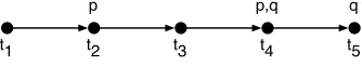
as times, and the relationR as the relation of temporal precedence (that is,Rww0 means that timewis earlier than timew0). Consider the graph in Figure 1. This shows a simple flow of time
t1 t2 t3 t4 t5
[image:5.612.215.382.468.499.2]p p,q q
Figure 1. A simple temporal model
consisting of five points. Here we will take the precedence relation to be the transitive closure of the next-time relation indicated by the arrows (after all, we think of the flow of time as transitive) thus every pointtiprecedes all points to its right. Note that (as we would expect from the internal perspective provided by modal languages) whether or not a formula is satisfied depends on where (or in this example, when) it is evaluated. For example, the formulas3(p∧q)is satisfied at points
t1,t2andt3(because all these points are to the left oft4where bothpandqare true together) but not att4andt5. On the other hand, becauseqis true att5, we have that3qis true att1,t2,t3and
t4. One special case is worth remarking on: note that for any basic formulaϕwhatsoever,2ϕ is satisfied att5. Why? Because the clause in the satisfaction definition for boxes says that2ϕ
is satisfied if and only ifϕis satisfied at allR-accessible points. As no points areR-accessible fromt5(it has no points to its right) this condition is trivially met.
its internal perspective. In languages such as English and Dutch, the default way of locating information temporally is to use tenses, and tenses locate information relative to the point of speech. For example, if at some timetI say “Clarence will fly”, then this will be true if at some future timet0 Clarence does in fact fly. Prior viewed tensed talk as fundamental: we exist in time, and have to deal with temporal information from the inside. He believed that the internal perspective offered by modal languages made it an ideal tool for capturing the situated nature of our experience and the context-dependent way we talk about it. Prior called his system tense
logic. He wrote F for the forward looking (or future) diamond, and had a second diamond, writtenP, for looking back into the past (so in Figure 1,P(p∧q)is true att5, for this point is to the right oft4, wherepandqare true together). Prior needed backward looking operators to mimic the effect of natural language past tense constructions; for further discussion of Prior’s work in this area, see Chapter 19 of this handbook.
Our next example brings us to one of the currently most influential ways of thinking about Kripke models; to view them as pictures of computational systems (we examine this perspec-tive in more detail in Section 6 when we discuss Propositional Dynamic Logic and the modal
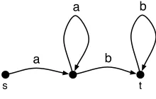
µ-calculus, and the computational interpretation underlies Chapters 12 and 17 of this handbook). Consider the graph shown in Figure 2. This shows a finite state automaton for the formal
lan-s t
a b
[image:6.612.298.408.342.412.2]a b
Figure 2. Finite state automaton foranbm(n, m >0)
guageanbm (n, m > 0), that is, for the set of all strings consisting of a non-empty block of
as followed by a non-empty block ofbs. But this is precisely the type of graph we can use to interpret a modal language. In this case it would be natural to work with a language with two di-amondshaiandhbi. Thehaidiamond will be used to explore thea-transitions in the automaton, while thehbidiamond explores theb-transitions. It follows that all formulas of the form
hai · · · haihbi · · · hbi>
(that is, an unbroken block ofhaidiamonds preceding an unbroken block ofhbidiamonds) are satisfied at the start nodes, for all modality sequences of this form correspond to the strings accepted by the automaton. Although simple, this example shows the key feature of many com-putational interpretations of modal logic: the relations are thought of as processes (here our processes are “read the symbola” and “read the symbolb”). Note that in this case we are think-ing in terms of deterministic processes (each relation is a partial function) but we could just as well work with arbitrary relations, which amounts to working with a non-deterministic models of processes, and we shall do so in Section 6.
q p s
q,p q
q,r q
e
Figure 3. Epistemic states of a simple agent
the agent’s current state, is markede. This represents the agents current knowledge (the agent knows thatqis the case). The other states represent the way the world might be. For example, although neitherpnorrare true in the current state, the agent views states in whichpandqare true together, and states in whichrandqare true together (but not states in whichpandqandr
are all true together) as epistemically acceptable alternatives to the current state. That is3(p∧q) (“p∧qis consistent with what the agent knows”) and3(r∧q)are both satisfied ate. Moreover 2q(“the agent knows thatq”) is satisfied ate, as at every epistemic alternative the information
qholds. Hintikka introduced the symbolKfor this usage of box (that is, he wroteKqfor “the agent knows thatq”) and his notation is still standard in contemporary epistemic logic. Epistemic logic is discussed in Chapters 18 and 20 of this handbook.
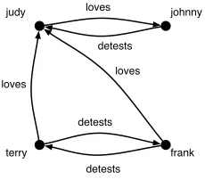
The next example is important for another reason. Modal logic is often viewed as an intrinsi-cally intensional logic, interpreted using possible world semantics. This view comes from what is probably the most historically influential interpretation of modal logic, namely as the logic of necessity and possibility. In this interpretation,3is read as “possibly”,2is read is “neces-sarily”, and the points of the Kripke model are regarded as possible worlds. Unfortunately, this interpretation has tended to overshadow the others, at least in certain research communities (some philosophers view modal logic, intensionality, and possible worlds as inextricably intermingled). To ensure that this illusion is dispelled, our last example will be completely extensional. Consider the graph in Figure 4.
loves
loves loves
detests
detests detests judy
terry frank
[image:7.612.241.356.522.623.2]johnny
Figure 4. Ordinary individuals
such situations. For example
hLOVESi> ∧ hDETESTSihLOVESi>
is true when evaluated at Terry: he loves someone and he detests someone who loves someone. Nowadays, modal logic is widely used for reasoning about such extensional situations. In par-ticular, the concept languages which lie at the heart of the description logics used in knowledge representation are often notational variants of (various kinds of) modal languages. Description logics are used in a wide range of applications for representing and reasoning about extensional information. They are treated in depth in Chapter 13 of this handbook.
We’re almost ready to define the standard translation, but before doing so let’s deal with three other matters. First, in most branches of logic and mathematics, there is a notion of two structures being isomorphic, which can be glossed as “mathematically indistinguishable”. Let’s take this opportunity to be precise about what isomorphism means in basic modal logic (we give the definition for models and frames with one relation; it generalises straightforwardly to structures with multiple relations).
DEFINITION 1 (Isomorphism). LetM= (W, R, V)andM0 = (W0, R0, V0)be models, and
f :W 7→W0 a bijection. If for allw, v∈W we have thatRwvif and only ifRf(w)f(v)then we say thatf is an isomorphism between the frames(W, R)and(W0, R0)and that these frames are isomorphic. If in addition we have, for all proposition lettersp, thatw ∈V(p)if and only iff(w)∈V0(p)then we say thatf is an isomorphism between the modelsMandM0and that these models are isomorphic.
As this definition makes clear, if modelsMandM0are isomorphic, each replicates perfectly the information in the other. Hence the following result is unsurprising:
PROPOSITION 2. Letf be an isomorphism between modelsMand M0. Then for all basic modal formulasϕ, and all pointswinM, we have thatM, w|=ϕif and only ifM, f(w)|=ϕ.
Proof. Immediate by induction on the construction ofϕ(see Lemma 9 for an example of such a
proof.) a
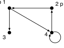
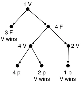
Second, we want to point out that it is possible to take a more dynamic perspective on the satisfaction definition. In particular, we can think of it as a game. Let’s start with a concrete example. Consider the model in Figure 5.
2 p p 1
[image:8.612.302.406.547.626.2]3 4
Figure 5. The formula323pis true at1and4, but false at2and3
a Falsifier (F), who disagree about the satisfiability of a formula in some model. The two player react differently to the connectives in the formula: for example, occurrences of disjunction allow V to make a choice as to which disjunct to verify, and force F to make both disjuncts false; negation switches the roles of the two players; and diamonds make V pick a successor of the current point, while boxes do the same for F. Moreover, for any propositional symbolp, V wins thep-game ifpis true at the current state, otherwise F wins. A player also wins the game if the other player must make a move for a modality but cannot.
3 F V wins
1 V
2 V 4 F
4 p 1 p
V wins 2 p
[image:9.612.233.365.249.389.2]V wins 4 V
Figure 6. Initial segment of a game tree
So let’s play the game for323pat1. Figure 6 shows (an initial segment of) the resulting game tree. Note that V can always win. Her most obvious option is to play3 in response to the outermost diamond; this leaves F with no possible response when faced with the task of falsifying23p. But V can also safely play4on her first move. As the tree shows, irrespective of F’s response, V can always reach a winning position. What this example suggests is completely general: for any modelM, pointw, and basic formulaϕ, we have thatM, w |=ϕif and only if V has a winning strategy when theϕ-game is played inMstarting atw.
2.2
The standard translation
We now understand what modal languages are, how they can be interpreted in graphs, and why this can be an interesting thing to do. What next? Well, if we were following a traditional path, we would probably remark that as modal languages are to be used for reasoning, some sort of proof system is called for. We might then point out that the set of all modal validities (that is, the
minimal modal logic) can be axiomatised by a Hilbert-style proof system called K. The axioms
of K are:
1. All propositional tautologies,
2. 2(ϕ→ψ)→(2ϕ→2ψ).
And there are two rules of proof: modus ponens (if` ϕand` ϕ → ψthen` ψ) and modal
generalisation (if ` ϕ then` 2ϕ). This looks like a standard axiomatisation of first-order logic with2behaving like∀. But K has no analogs of the first-order axioms with tricky side conditions on freedom and bondage of variables, such as∀xϕ→[t/x]ϕ. This is no coincidence. As the standard translation given below will make clear, modal logic is essentially a perspicuous variable-free notation for a fragment of first-order logic.
But proof systems are not our goal. This chapter is concerned with semantic issues, so quite different aspects of modal logic call for our attention. To get the ball rolling, let’s return to our basic semantic entities (Kripke models) and ask what they actually are. This will provide a point of entry to one of the main themes of the chapter: the relationship between modal and classical logic.
So what is a Kripke model? No mystery here. A Kripke model(W,{Rm}
m∈MOD, V)is what
model theorists call a relational structure. That is, we have a domain of quantificationW, a collection of binary relations over this domain, and a collection of unary relations as well (after all,V(p)is a unary relation for eachp∈PROP). But this means that we are not forced to talk about Kripke models using modal languages: they provide us with everything needed to interpret classical languages too. For example, to talk about a model(W,{Rm}
m∈MOD)using first-order
logic we would simply make use of a first-order language with a binary relation symbolRmfor everym∈MOD, and a unary relation symbolP for everyp∈PROP. Modal logicians have a name for this language: they call it the first-order correspondence language (for the basic modal language over PROP and MOD).
Why “correspondence language”? Because every basic modal formula (in the language over PROP and MOD) corresponds to a first-order formula from this language via the standard
trans-lation:
STx(p) = P x STx(⊥) = ⊥ STx(¬ϕ) = ¬STx(ϕ) STx(ϕ∧ψ) = STx(ϕ)∧STx(ψ)
STx(hmiϕ) = ∃y(Rmxy∧STy(ϕ)) STx([m]ϕ) = ∀y(Rmxy→STy(ϕ)).
earlier that diamonds and boxes were essentially a simple macro notation encoding quantification over accessible states; the standard translation expands these macros. Note thatSTx(ϕ)always contains exactly one free variable (namely x). This free variable is what allows the internal perspective, typical of modal logic, to be mirrored in a classical language: assigning a value to this variable is analogous to evaluating a modal formula inside a model at a certain point.
Here’s an example of the translation at work:
STx(p→3p) = STx(p)→STx(3p) = P x→STx(3p)
= P x→ ∃y(Rxy∧STy(p)) = P x→ ∃y(Rxy∧P y).
As the reader can easily check,p→3pand its standard translationP x→ ∃y(Rxy∧P y)are equisatisfiable in the following sense: for any modelM, and any pointwinM, we have that
M, w |= p → 3pif and only if M |= P x → ∃y(Rxy ∧P y)[x ← w], where the notation [x← w]means assignwto the free variablex. Unsurprisingly, this relationship is completely general:
PROPOSITION 3. For any basic modal formulaϕ, any modelM, and any pointwinMwe have thatM, w|=ϕiffM|=STx(ϕ)[x←w].
Proof. There is practically nothing to prove. The clauses of the standard translation mirror the
clauses of the satisfaction definition. Hence the result is immediate by induction on the structure
of modal formulas. a
Thus the standard translation gives us a bridge between modal logic and classical logic. And we can immediately use this bridge to transfer meta-theoretic results for first-order logic to modal logic.
PROPOSITION 4. Basic modal logic has the compactness property. That is, if Σis a set of basic modal formulas, and every finite subset of Σis satisfiable, then Σ itself is satisfiable. Moreover, basic model logic has the L¨owenheim-Skolem property. That is, if a set of basic modal formulasΣis satisfiable in at least one infinite model, then it is satisfiable in models of every infinite cardinality.
Proof. We show that basic modal logic has the L¨owenheim-Skolem property. Suppose that Σ is a set of basic modal formulas that has at least one infinite model. Let STx(Σ)be the set of (first-order) formulas obtained by standardly translating all the formulas inΣ. Now, asΣhas an infinite model, by Proposition 3 so doesSTx(Σ). But first-order logic has the L¨owenheim-Skolem property, henceSTx(Σ)has a model of every infinite cardinality. But, again by appeal to Proposition 3, each of these models satisfiesΣ, so basic modal logic has the L¨owenheim-Skolem property too. The argument showing it has the compactness property is similar. a
Another easy consequence of the standard translation is that the set of validities (in basic modal languages) is recursively enumerable. For a basic modal formulaϕis valid iffSTx(Σ)is a first-order validity, and the set of first-order validities is recursively enumerable.
modal syntax, means that propositional modal logic is an attractive tool for certain applications. Moreover, viewed as a tool for talking about models, any basic model language can be regarded as a fragment of its corresponding first-order language: the standard translation systematically maps modal formulas to first-order formulas (in one free variable) and makes the quantification over accessible states explicit. This allows us to quickly establish some basic modal meta-theory by appeal to known results for first-order logic.
3 BISIMULATION AND DEFINABILITY
With the basics behind us it is time to look deeper. In particular, it is time to start mapping the expressive strengths and weaknesses of the basic modal language. Now, the expressive power of a language is usually measured in terms of the distinctions it can draw. A language with just the two expressions “like” and “dislike” would provide only the roughest possible classification of the world, whereas a richer language of assent and dissent would make it possible to draw finer distinctions inside the accepted and rejected situations. So what distinctions can modal languages draw? In this section we discuss this question at the level of models, and in Section 5 we shall reconsider it at the level of frames. In what follows it will often be useful to think in terms of
pointed models. That is, we shall often present models together with an explicit distinguished
point to indicate where we are trying to find a difference.
3.1
Drawing distinctions
A modal language (and indeed any logical language whose formulas form a set) can distinguish between some models(M, s)and(N, t), but not between all such pairs. For example, our basic modal language can distinguish the pair of models shown in Figure 7 (in these graphs all points are irreflexive).
[image:12.612.285.417.463.572.2]s t
Figure 7.MandNare modally distinguishable.
Here2(2⊥ ∨32⊥)is a modal formula that distinguishes these models: it is true inMat
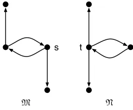
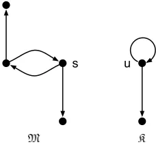
s, but false inNatt. But now consider the pair of models shown in Figure 8 (in these graphs,u
is reflexive, and all other points are irreflexive). Is it possible to modally distinguish(M, s)from (K, u)? That is, is it possible to find a (basic) modal formula that is true inMats, but false inK
s u
Figure 8.MandKare not modally distinguishable.
Rxxis not satisfiable (under any variable assignment) in modelM, but it is satisfied inKwhen
uis assigned tox. But no matter how ingenious you are, are you will not find any formula in the basic modal language that distinguishes these models at their designated points. Why is this?
3.2
Bisimulation
A natural approach to this question is to consider its dual: when should two models be viewed as modally identical? For example, given a process interpretation, when would we view two transition diagrams as representations of the same process? The model MandKof Figure 8 provide an intuitive example: they seem to stand for the same process when we look at possible actions and deadlocks. At each live stage, the process can enter a deadlock situation. By contrast,
MandNin Figure 7 are different, as not every state inNis threatened with immediate dead-lock. Or consider the epistemic interpretation: when would we want to say that two graphs represent the same epistemic information? For example we would probably want to identify the two epistemic models shown in Figure 9 at their distinguished pointssandt.
q p s
p
t q
q p
Figure 9. Two epistemically equivalent models.
The modal logician’s idea of asking when two distinct structures are modally identical (that is, make the same modal formulas true) lies within an older (and broader) tradition of looking for the structure preserving morphisms in a given mathematical domain, and letting the corresponding theory describe those notions that are invariant for such morphisms. This is the spirit of Klein’s Program in geometry, proposed around 1870, and still influential in many fields. Of course, there is no unique answer to the question of when two structures are the same. This insight was stated forcefully in recent years by President Clinton during the Lewinsky hearings: It all depends on
what you mean by “is”. Clinton’s Principle for modal logic means that we should first try to
stip-ulate some notion of structural equivalence for models that is appropriate for modal languages. This is the purpose of the following definition (first formulated in van Benthem [116, 119]). We state it here for models with one relationR, but the definition generalises straightforwardly to models with any number of relations.
DEFINITION 5 (Bisimulation). A bisimulation between modelsM = (W, R, V)andM0 = (W0, R0, V0)is a non-empty binary relationEbetween their domains (that is,E ⊆W ×W0) such that wheneverwEw0we have that:
Atomic harmony:wandw0satisfy the same proposition symbols,
Zig: ifRwv, then there exists a pointv0(inM0) such thatvEv0andR0w0v0, and
Zag: ifR0w0v0, then there exists a pointv(inM) such thatvEv0andRwv.
If there is a bisimulation between two modelsMandN, then we say thatMandNare bisimilar. Moreover, we say that two states are bisimilar if they are related by some bisimulation.
Putting this in words: two states are bisimilar if they make the same atomic information true and if, in addition, their transition possibilities match. That is, if a transition to a related state is possible in one model, then the bisimulation must deliver a matching transition possibility in the other. Atomic harmony coupled with the matching transitions concept embodied in the zigzag clauses make bisimulation a natural notion of process equivalence, and indeed bisimulations were independently discovered in computer science (see Park [90]).
Returning to the modelsM,K, andNconsidered above (and disregarding proposition sym-bols) it is easy to see that MandK are bisimilar: the dotted lines in Figure 10 indicate the required bisimulation (note that the indicated bisimulation links the two designated points). Fur-thermore, it is easy to see that there is no bisimulation that links the designated points ofNand
K. Why not? Because a move fromtto the right-hand world inNhas no matching move inK: moving downwards fromuis no option (end-points never bisimulate with points having succes-sors) but neither is moving reflexively fromuto itself (as one can move fromuto a successor which is an endpoint, but this can’t be done from the right-hand world inN).
Given any modal modelM, bisimulations can be used in at a number of ways. The so-called
s u t
Figure 10.MandKare bisimilar,KandNare not.
also all aesthetic symmetries. (A butterfly is a redundant object, as one wing contains enough information under this perspective.)
But bisimulations can also be used to make bigger models: one important construction which does this is called tree unraveling (for a very early paper using this construction, see Dummett and Lemmon [31]; for an influential paper that made heavy use of it, see Sahlqvist [100]).
To unravel a model we take all finite R-sequences of points in Mthat start at some point
w. These sequences form a tree with one-step extensions of sequences as the tree-successor relation. Projection from a sequence to its last element is a bisimulation onto the originalM. As an example, consider the unraveling of two element modelKaround its distinguished point
uto the infinite comb-like structure shown in Figure 11 (we usevas the name of the other point in this model). Reasoning about trees is often easier than reasoning about arbitrary graphs, and
<u> <u,v>
<u,u> <u,u,v>
<u,u,u> <u,u,u,v>
. . .
Figure 11. UnravelingKaroundu.
[image:15.612.227.370.472.631.2]section, tree unraveling is relevant to the decidability of modal logic.
Three other model constructions used in modal logic, namely disjoint unions, generated
sub-models, and bounded morphisms (or p-morphisms) are also bisimulations. Historically, all three
constructions were widely used in modal logic more than a decade before the unifying concept of a bisimulations was introduced (the classic source for these constructions is Segerberg [102], where they are heavily used, often in combination, to prove completeness theorems). All three constructions are fundamental tools in many areas of modal logic (for example, when reformu-lated at the level of frames, they are key ingredients in the Goldblatt-Thomason Theorem which we discuss in Section 5) so we take this opportunity to define them for models with one accessi-bility relation. These definitions generalise straightforwardly to models of arbitrary signature.
The simplest construction is forming disjoint unions. If we have a pair of disjoint models (that is a pair of models(W, R, V)and(W0, R0, V0)such thatW andW0are disjoint) then their disjoint union is the model(W∪W0, R∪R0, V +V0), whereV +V0is the valuation defined byV +V0(p) =V(p)∪V0(p), for all proposition symbolsp. That is, forming a disjoint union of two models means lumping together all the information in the two graphs. What if the graphs are not disjoint? Then we simply take disjoint isomorphic copies of the two models, and form the disjoint union of the copies. This lumping together process can be generalised to arbitrarily many models, which prompts the following definition.
DEFINITION 6 (Disjoint Unions). Given mutually disjoint modelsMi = (Wi, Ri, Vi), where
iranges over the elements of some index set I, we define the disjoint union of these models to beM = (W, R, V), whereW = S
i∈IWi,R =Si∈IRi, andV(p) = Si∈IVi(p)for all proposition symbolsp. To form the disjoint union of a collection of models that are not mutually disjoint, we first take mutually disjoint isomorphic copies, and then form the disjoint union of the copies.
It is immediate from this definition that any component modelMi of a disjoint unionMis bisimilar withM: for the bisimulation relationEwe simply take the identify relation. Identity clearly satisfies the atomic harmony and zigzag conditions required of bisimulations.
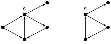
Disjoint unions build bigger models from (collections of) smaller ones. Generated submodels do the reverse. They arise by restricting attention to subgraphs of a given graph that are closed under relational transitions. For example, consider the two graphs in Figure 12.
[image:16.612.263.442.505.577.2]s s
Figure 12. Generating a submodel froms.
It is clear that the graph on the right arises by restricting attention to a certain transition-closed subgraph of the graph on the left, namely the set of point reachable by taking sequences of transitions froms. This motivates the following definition.
DEFINITION 7 (Generated Submodels).
V0(p) =V(p)∩W0. We say thatW0isR-closed if for allu∈W0, ifRuvthenv∈W0. Finally, we say thatM0is a generated submodel ofMiffM0is the restriction ofMto anR-closed subset ofW.
IfM0 = (W0, R0, V0)is a generated submodel ofM = (W, R, V), andS ⊆ W0 has the property that everyw0∈W0is reachable via a finite sequence ofR-transitions from somes∈S, then we say thatM0 is the submodel ofMgenerated byS. IfSis a singleton set{s}, then we say thatM0is the submodel ofMgenerated by the points.
A generated submodel is bisimilar to the model that gave rise to it: as with disjoint unions, the identity relation relates the two models in the appropriate way. Incidentally, note that every component model of a disjoint union is a generated submodel of the disjoint union.
Finally we turn to bounded morphisms (orp-morphisms as they are often called).
DEFINITION 8 (Bounded Morphisms).
A bounded morphism between modelsM= (W, R, V)andM0= (W0, R0, V0)is a function
f with domainW and rangeW0such that:
Atomic harmony: Points inW and theirf-images satisfy the same proposition symbols (that is,w∈V(p)ifff(w)∈V0(p), for all proposition symbolsp).
Morphism: ifRwv, thenR0f(u)f(v).
Zag: ifR0w0v0, then there exists av(inM) such thatf(v) =v0andRwv.
Iffis a bounded morphism fromMtoM0andfis surjective, then we say thatM0is a bounded morphic image ofM.
Bounded morphisms are bisimulations: a bounded morphism is simply a bisimulation in which the bisimulation relation E is an R-preserving morphism f (note that the only essen-tial difference between the two definitions is that the morphism clause replaces the zig clause, and clearly morphism implies zig). Historically, it was the definition of bounded morphisms that inspired the definition of bisimulations.
As an example of a bounded morphism between models, consider Figure 13 (again we ignore proposition symbols).
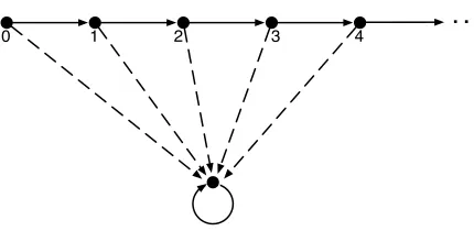
[image:17.612.189.404.501.611.2]0 1 2 3 4 . . .
Figure 13. Bounded morphism collapsing the natural numbers to a reflexive point.
3.3
Invariance and definability in first-order logic
Structural invariances preserve certain patterns definable in appropriate languages. Before pur-suing the match between bisimulation and modal logic, let us examine the situation in first-order logic. The archetypal structural invariance is isomorphism between models. As we saw ear-lier (recall Proposition 2) modal formulas are invariant for isomorphism. More generally, it is well known that if f is an isomorphism betweenMandN, then for each first-order formula
ϕ(x1, . . . , xk), and each matching tuple of objectshd1, . . . , dkiinM, the following equivalence holds:
M|=ϕ[d1, . . . , dk] iff N|=ϕ[f(d1), . . . , f(dk)],
or stated in words: first-order formulas are invariant for isomorphism.
On special models, the converse also holds. For example, it is a well-known fact that any two finite models with the same first-order theory are isomorphic. But no general converse holds, as there are many more isomorphism classes of models than complete first-order theories. Invariance for isomorphism is even a defining condition for any logic in abstract model theory. But no matter how strong the logic, the converse still fails whenever the formulas of a logic form a set, as opposed to the proper class of isomorphism types.
Thus it makes sense to look at invariance conditions for weaker notions of structural equiva-lence. For example, a potential isomorphism between two modelsMandNis a non-empty setI
of finite partial isomorphisms satisfying the back-and-forth extension conditions that, whenever
f ∈ I andd ∈ M, then there is ane ∈ N such thatf ∪ {(d, e)} ∈ I, and vice-versa. Note that isomorphisms induce potential isomorphisms: simply takeI to be the family of all finite restrictions. The converse is not true. Matching up all finite sequences of rational numbers with equally long sequences of real numbers (in the same order) is a potential isomorphism between
QandR, even though these two structures are not order-isomorphic for cardinality reasons.
It is easy to show that all first-order formulas are invariant for potential isomorphism, but the real match is with a stronger language: two models are potentially isomorphic iff they have the same complete theory in the infinitary first-order logicL∞ω. This formalism also gives rise to much stronger definability results. For example, for each modelMthere is a sentenceδM of
L∞ωwhich holds only in those modelsNwhich have a potential isomorphism withM; that is, models can be defined up to potential isomorphism. Moreover, countable models can even be defined (modulo isomorphism) using only countable conjunctions and disjunctions. This is all very nice of course, but infinitary logic is a bit outlandish from a practical viewpoint.
Better matches between structural invariance and first-order definability arise in the more fine-grained setting of Ehrenfeucht-Fra¨ıss´e comparison games between modelsMandNplayed between a Spoiler (who looks for differences between the models) and a Duplicator (who looks for analogies between them). ModelsMandNhave the same first-order theory up to quantifier depthkiff the Duplicator has a winning strategy in their comparison game overkrounds. We forgo the details here, as we will define a modal comparison game of this sort at the end of the section.
3.4
Invariance and definability in modal logic
With these analogies in mind, let us now investigate the modal situation. For a start, modal formulas are invariant for bisimulation:
LEMMA 9 (Bisimulation Invariance Lemma). IfEis a bisimulation betweenM= (W, R, V)
Proof. By induction on the construction of modal formulas. The case for proposition symbols
is immediate by atomic harmony. The inductive steps for the boolean connectives are straight-forward. And the inductive step for 3formulas shows exactly what the zigzag clauses were designed for. For consider the left to right direction. GivenM, w|=3ϕandwEw0, we want to show thatM0, w0 |=3ϕ. Now,M, w |= 3ϕmeans that there is somev inMsuch thatRwv
andM, v|=ϕ. But then (by zig) there must be a pointv0inN0such thatvEv0andR0w0v0. By the induction hypothesis,M0, v0 |=ϕ, henceM0, w0 |= 3ϕas required. The argument for the right to left direction is essentially the same, using zag in place of zig. a
The result allows us to show failures of bisimulation easily. For example, we have already sketched an argument showing that the models N and K of Figure 10 have no bisimulation between their designated points, but a quicker proof is now possible: these points cannot be bisimilar because there are modal formulas (for example2(2⊥ ∨32⊥)) which are satisfied at one point but not the other. On the other hand, the dotted lines in Figure 10 show thatMand
Kare bisimilar; it follows that all points linked by a dotted line in these graphs make exactly the same modal formulas true. Another typical application of this result is to show the undefinability of certain structural notions. For example, we can show that irreflexivity is modally undefinable: no modal formula holds in exactly those pointswof models such that¬Rww. To prove this, it suffices to find two bisimilar points in two models, one of which is reflexive, the other irreflex-ive. One such example is the bisimulation between the designated points ofMandKshown in Figure 10. Another is the bounded morphism of Figure 13 which collapses the natural numbers to a single reflexive point.
Another consequence of this result is that the disjoint union, generated submodel, and bounded morphism constructions are all satisfaction preserving. More precisely:
LEMMA 10. Modal satisfaction is invariant under the formation of disjoint unions, generated submodels, and bounded morphisms. That is:
1. IfM= (W, R, V)is the disjoint union ofMi= (Wi, Ri, Vi), forifrom some index setI, then for allw∈Wiand alli∈Iwe have thatM, w|=ϕiffMi, w|=ϕ.
2. IfM0 = (W0, R0, V0)is a generated submodel ofM= (W, R, V), then for allw0∈W0
we have thatM, w0 |=ϕiffM0, w0 |=ϕ.
3. IfM0 = (W0, R0, V0)is a bounded morphic image ofM= (W, R, V)under the bounded morphismf, then for allw∈W we have thatM, w|=ϕiffM0, f(w)|=ϕ.
Proof. All three results could be proved by induction on the structure onϕ. But such proofs are unnecessary: we know that disjoint unions, generated submodels, and bounded morphisms are all examples of bisimulations, hence these results follow from Lemma 9. a
To sum up the discussion so far, bisimulation implies modal equivalence. But what about the converse? For finite models, we have the following.
PROPOSITION 11. If pointswandw0from two finite modelsMandNsatisfy the same modal formulas, then there is a bisimulationEbetweenMandNsuch thatwEw0.
Proof. Assume we are working with models containing only a single relationR. We will show that the relation of modal equivalence is itself a bisimulation. That is, we will define the bisimu-lation rebisimu-lationEbywEw0iffwandw0make the same modal formulas true. We now verify that
It is immediate thatE satisfies atomic harmony. As for zig, assume thatwEw0 andRwv. Assume for the sake of contradiction that there is nov0 inM0 such thatR0w0v0 andvEv0. Let
S0 ={u0 | R0w0u0}. Now, aswhas anR-successorv, we haveM, w |=3>. AswEw0, we haveM0, w0 |=3>too, henceS0is non-empty. Furthermore, asM0is finite,S0 must be finite too, so we can write it as{u01, . . . , u0n}. By assumption, for everyu0i∈S0there exists a formula
ψisuch thatM, v|=ψibutM0, u0i 6|=ψi. It follows that
M, w|=3(ψ1∧ · · · ∧ψn) and M0, w06|=3(ψ1∧ · · · ∧ψn),
which contradicts our assumption that wEw0. HenceE satisfies zig. A symmetric argument shows thatEsatisfies zag too, hence it is a bisimulation. a
Thus on finite models, the expressive power of modal languages matches up exactly with bisimulation invariance. This result can be extended to broader model classes, such as models with finite branching width for successors (note that the proof just given does not depend on the models involved being finite: it would also work for infinite models in which each point has only finitelyy manyR-successors) and suitably saturated models in a model-theoretic sense. But no general converse can hold, for the reason mentioned earlier for first-order logic. Indeed, the converse does not hold generally even for countable models: not all modally equivalent countable models are bisimilar. The two models in Figure 14 satisfy the same modal formulas at their roots, but if there were a bisimulation between them, the infinite chain on the right would also have to occur on the left.
. . . .
[image:20.612.292.411.397.438.2]...
Figure 14. Modally equivalent but not bisimilar.
This counterexample can be repaired by passing to an infinitary modal languageL∞ωwith ar-bitrary (countable) conjunctions and disjunctions. Infinitary modal equivalence occurs between countable models(M, s)and(N, t)whenever there is a bisimulation linkingstot. Furthermore, every countable model(M, s)is defined up to bisimulation by someL∞ωformulaδM,s. Again, such infinitary languages are somewhat impractical, but there are some useful bisimulation in-variant formalisms which lie between the basic modal language and its infinitary extension. Two example are propositional dynamic logic and the modalµ-calculus, which are discussed in
Sec-tion 6.
Lemma 9 and its partial converses do not exhaust what needs to be said about the role played by bisimulations in modal model theory. But to gain a deeper understanding, we need to bring in a third component: the first-order correspondence language. Let’s do this right away,
3.5
Modal logic and first-order logic compared
the converse does not hold: some first-order formulas in the correspondence language are not modally definable. We have already see an example. As the bisimulation between modelsMand
Kshows (recall Figure 10) no modal formula defines¬Rxx. Thus, viewed as a tool for talking about models, modal logic is strictly less expressive than the full first-order correspondence language. And this prompts a further question: given that a modal language is essentially a fragment of the corresponding first-order language, exactly which fragment is it? This question has an elegant answer. First, a preliminary definition.
DEFINITION 12. A first-order formulaϕ(x)is invariant for bisimulation if for all modelsM
andM0, and all pointswinMandw0inM0, and all bisimulationsEbetweenMandM0such thatwEw0, we have thatM|=ϕ[x←w]iffM0|=ϕ[x←w0].
We can now state the main result: basic modal languages correspond to the fragment of their first-order correspondence language that is invariant for bisimulation. More precisely:
THEOREM 13 (Modal Characterisation Theorem). The following are equivalent for all
first-order formulasϕ(x)in one free variablex:
1. ϕ(x)is invariant for bisimulation.
2. ϕ(x)is equivalent to the standard translation of a basic model formula.
Proof. That clause (ii) implies (i) is a more or less immediate consequence of Lemma 9. The
hard direction is showing that clause (i) implies (ii). The original proof can be found in van Benthem [116, 119]. Two other proofs are given in Chapter 5 of this handbook. One is quite close to van Benthem’s original approach, the other is based on games. a
Nowadays many different proofs are known for this result, and for various extensions and variants. For example, Rosen [98] showed that the result holds over finite models; this is far from obvious, as the restriction to finite models means that many standard results of first-order model theory (such as the Compactness Theorem) cannot be applied. And Otto [89] showed that the modal equivalent guaranteed to exist by clause (ii) of the previous theorem can be restricted to a formula of modal operator depth2k, wherekis the quantifier depth ofϕ(x).
Basic modal logic and first-order logic are analogous in many ways. As we mentioned in Section 2, via the standard translation modal logic immediately inherits basic meta-theoretic properties of its more powerful neighbour, such as the Compactness and L¨owenheim-Skolem Theorems. But not all such transfer is automatic. Consider, for example, the Craig Interpolation property:
Ifϕ|=ψthen there exists a formulaθwhose vocabulary is included in that of both
ϕandψsuch thatϕ|=θandθ|=ψ.
Does the same result hold for basic modal formulasϕandψsuch thatϕ|=ψ? Appealing to the result for first-order logic gives us a first-order formulaθsuch thatSTx(ϕ)|=θandθ|=STx(ψ). But what guarantees that this interpolant is modally definable? Interpolation does in fact hold for the basic modal language, but additional work is needed to prove this. However interpolation does mesh well with the above preservation results (for a detailed account, see Chapter 8). Here is an improvement on the Modal Characterisation Theorem. We say that a first-order formulaϕ
impliesψalong bisimulation if the following implication holds: ifEis a bisimulation between (M, s)and(N, t), andM, s|=ϕ, thenN, t|=ψ.
1. ϕ(x)impliesψ(x)along bisimulation.
2. There is a modally definableθin the common vocabulary ofϕandψsuch thatϕ|=θand
θ|=ψ.
Proof. The proof can be found in Barwise and van Benthem [11]. Note that the Modal
Charac-terisation Theorem follows by takingϕ(x)equal toψ(x). This result does not imply ordinary modal interpolation as it stands: additional work is again needed. a
Behind the above observations is the fact that the cheaply transferred properties are universal in some sense, whereas the universal-existential property of interpolation requires honest work. Even so, there is an intuition (based on decades of positive experience with transferring results) that modal logic and first-order logic share all general meta-properties except decidability. No proofs of significant formulations of this idea have been found so far, but we can point to some broad analogies regarding methods. Generally speaking, bisimulation plays the same role for modal logic that potential isomorphism does for first-order logic. This can even be made precise in the following sense. To each first-order modelMwe can associate a modal model whose points are the variable assignments intoM, and whose accessibility relations are changes from one assignmentgto anotherg(x:=d)that resets the value for the variablexto the objectd∈M. Then two modelsMandNhave a potential isomorphism between them iff their associated modal models are bisimilar; see van Benthem [124] for details.
We conclude this discussion with two general transfer results that allow us to switch between modal and first-order relations between models. In essence, both results have the form of a commutative diagram.
LEMMA 15 (First Lifting Lemma). The following are equivalent for all models(M, s) and
(N, t):
1. (M, s)and(N, t)are modally equivalent.
2. (M, s)and(N, t)have elementary extensions to models(M+, s)and(N+, t)which are
bisimilar.
LEMMA 16 (Second Lifting Lemma). The following are equivalent for all models(M, s)and
(N, t):
1. (M, s)and(N, t)are modally equivalent.
2. (M, s)and (N, t)are bisimilar to models(M+, s)and(N+, t)which are elementarily
equivalent.
Proof. The first lifting lemma was originally proved in van Benthem [116]. It is the key item in
(some proofs of) the Characterisation Theorem (the+-models are suitably saturated elementary extensions which allow the Characterisation Theorem to be proved rather straightforwardly). The second lifting lemma (see van Benthem [122] for the original result, and Andr´eka, van Benthem, and N´emeti [5] for full proof details) involves judicious tree unraveling of the two models, dupli-cating sub-trees to create uniformity, coupled with an Ehrenfeucht-Fra¨ıss´e argument to establish
3.6
Bisimulation as a game
We have said that bisimulation is a sort of process equivalence. The dynamic character of the notion can be brought out by viewing it as a game. Consider a game between Spoiler (the difference player) and Duplicator (the analogy player) and comparing successive pairs in two pointed model(M, w)and(N, w0):
If wand w0 do not agree on atomic information, Spoiler wins the game in zero rounds. In subsequent rounds, Spoiler chooses a state in one model which is a suc-cessor of the currentworw0, and Duplicator responds with a matching successor in the other model. If the chosen points differ in their atomic properties, Spoiler wins. If one player cannot move, the other wins. Duplicator wins on infinite runs on which Spoiler does not win.
This game captures the zigzag behaviour of bisimulations in an obvious sense. It is also
determined: one of the two players has a winning strategy. (This is because it is an open
Gale-Stewart game in the sense of game theory.) For example, returning yet again to the modelsM,N
andKconsidered at the start of this section, we see that Duplicator has a winning strategy in the comparison game for the modelsMandKstarting from their matched designated points, while Spoiler has one forMandN. The following result clarifies the role of these games precisely:
LEMMA 17 (Adequacy of Modal Comparison Games).
1. There is an explicit correspondence between Spoiler’s winning strategies in a k-round comparison game between(M, s)and(N, t)and modal formulas of modal operator depth
kon whichsandtdisagree.
2. There is an explicit correspondence between Duplicator’s winning strategies over an infinite-round comparison game between(M, s)and(N, t)and the set of all bisimulations be-tweenMandNthat link the pointssandt.
Proof. This result is essentially a fine-grained restatement of the Lemma 9 from a game-theoretic
perspective. See Chapter 5 of this handbook for more on game-based approaches to bisimulation. a
For example, in the game between the modelsMandK given earlier, Duplicator wins by choosing responses that stick to the bisimulation links. And in the game betweenMandN, Spoiler can win in at most three rounds by using the earlier modal difference formula2(2⊥ ∨ 32⊥)of modal operator depth three. In each round he can make sure that some modal difference remains at the current match, with the modal operator depth descending each time.
4 COMPUTATION AND COMPLEXITY
We view modal logic as a tool for representing and reasoning about graphs. Our discussion of expressivity has given us some insight into the representational capabilities of modal logic (at least at the level of models) but what about reasoning?
Before going further, two general remarks. First, although we are about to study reasoning, we are not about to embark on the study of modal proof systems (apart from anything else, the standard proof systems are only relevant to satisfiability and validity checking, and there is more to modal reasoning than this). Secondly, although we are ostensibly moving on from expressivity issues to computational issues, the two topics are intertwined. In essence, the positive computa-tional results reported here arise from negative expressivity results (for example, the inability of the basic modal language to force the existence of infinite models).
4.1
Model checking
The model checking task can be formulated locally:
Given a (finite) model M, a point w inM, and a basic modal formulaϕ, is ϕ
satisfied inMatw?
Or globally:
Given a (finite) modelM, and a basic modal formulaϕ, isϕsatisfied at all points inM?
Or in a form that subsumes both the local and global perspectives:
Given a (finite) modelM, and a basic modal formulaϕ, return the set of points in
Mthat satisfyϕ.
In what follows we shall work with the last formulation, which is probably the most common way of thinking about model checking in practice.
Now, model checking is clearly a task with computational content — but is it really a
reason-ing task? In our view, yes. In essence, a model is a ‘flat’ store of information: it consists of a
collection of entities, together with a specification of which entities have which properties, and which entities are related by which atomic relations. A modal formula, on the other hand, is a recursively constructed tree. The embedding of connectives and modalities within one another permits relatively short formulas to make interesting assertions, assertions that go way beyond the mere listing of atomic facts. If we add to these differences the practical observation that in typical applications the formula will be much smaller than the model, we see that model checking is about synchronising two very different forms of information: it tells us whether the abstract information embodied in the formula is implicitly present in the model, and gives us set of points where this implicit information emerges. Viewed this way, model checking is a quintessential reasoning task.
(for example, absence of deadlock) then by checking the formula in the model we can determine whether the chip is well-designed or not.
So how should we perform model checking? The standard approach is to use a bottom-up
labeling algorithm. To model check a formulaϕwe label every point in the model with all the subformulas ofϕthat are true at that point. We start with the proposition symbols: the valuation tells us where these are true, so we label all the appropriate points. We then label with more complex formulas. The booleans are handled in the obvious way: for example, we labelwwith
ψ∧θifwis labeled with bothψandθ. As for the modalities, we labelwwith3ϕif one of its
R-successors is labeled withϕ, and we label it with2ϕif all of itsR-successors are labeled with
ϕ. The beauty of this algorithm is that we never need to duplicate work: once a point is labeled as makingϕtrue, that’s it. This makes the algorithm run in time polynomial in the size of the input formula and model: the algorithm takes time of the order of
con(ϕ)×nodes(M)×nodes(M),
where con(ϕ)is the number of connectives inϕ, and nodes(M)is the number of nodes inM. Thus modal model checking is a computationally tractable task, but this is not the case for first-order logic. In fact, model checking first-first-order formulas is a PSPACE-complete task (see Chan-dra and Merlin [20]). That is, although it is possible to write an algorithm that solves the first-order model checking task using an amount of computer memory that is only polynomial in the size of the input model and formula, the algorithm may require running time that is exponential in the size of the input. The problem, of course lies with the quantifiers. Given that the stan-dard assumptions made in complexity theory are correct, there is no way of adapting the labeling algorithm (or indeed, any other algorithm) to perform first-order model checking in polynomial time.
However the labeling algorithm sketched above does adapt to more powerful modal languages, and this is important. As we said above, when model checking we want to state interesting high-level properties of the situation we are modeling, and often the ordinary 2and3modalities simply aren’t expressive enough. Far more useful is the binary Until modality:
M, s|=U(ψ, θ) iff there is atsuch thatsR∗tandM, t|=ψ,
and for allusuch thatsR∗uanduR+twe haveM, u|=θ.
(HereR∗is the reflexive transitive closure of an irreflexive accessibility relationR, andR+is its transitive closure.) The Until modality (which comes in several related forms) is a fundamental component of some of the most important formalisms used in model checking, such as LTL (Linear Time Temporal Logic) and CTL (Computational Tree Logic). For a introduction to these logics from a model checking perspective, see Clarke, Grumberg and Peled [23].
Now, we shall discuss the Until operator, and why it is useful, in Section 6.3. Here we simply want to address the following question: how do we extend the labeling algorithm to handle formulas of the formU(ψ, θ)? Here’s the basic idea. First, if any pointwis labeled withψ, label
wwithU(ψ, θ). Second, if any pointv is labeled withθand at least oneR-successor ofvis labeled withU(ψ, θ), then labelvwithU(ψ, θ). It should be clear that these two steps correctly reflects the semantics for Until just given. Moreover, it can be made algorithmically precise as the pseudo-code given in Figure 15 shows.
procedureCheckU(ψ, θ)
T :={v|ψ∈label(v)};
for allw∈Tdo
label(w) =label(w)∪ {U(ψ, θ)};
end for all ; whileT 6=∅do
choosew∈T ;
T :=T\ {w};
for allvsuch thatRvwdo
ifU(ψ, θ)∈/ label(v)andθ∈label(v)then label(v) :=label(v)∪ {U(ψ, θ};
T :=T∪ {v};
end if ; end for all ; end while ; end procedure
Figure 15. Model checkingU(ϕ, θ)
nowadays it seems safe to assume that most readers of a technical book on logic have at least a nodding acquaintance with programming (indeed, we suspect that most of our readers would find it straightforward to devise a computational syntax for models and modal languages, and to implement simple programs for working with them).
Nonetheless, such issues cannot be taken lightly. A major factor in the spectacular progress of model checking has been the development of Binary Decision Diagrams (BDDs) and Ordered
Binary Decision Diagrams (OBBDs). BDDs (which are compact representations of boolean
expressions) were introduced by Lee [80] and Akers [3], and OBBDs (a more sophisticated form of BDD with fewer representational redundancies) were introduced by Bryant [16]. BDDs were first proposed for model checking by Burch, Clarke, McMillan, Dill, and Hwang [17] and as the title of this paper indicates (“Symbolic model checking: 1020states and beyond”) this lead to a dramatic increase in the size of the models that could be handled. It is important not to underestimate the gap between the labeling algorithm sketched above, and what it takes to make a working model checker handle a large model. Crossing this gap requires a combination of theoretical insight and computational expertise, and an entire research community is devoted to exploring the issues involved.
For a good textbook level introduction to model checking, see Huth and Ryan [65]. This book not only introduces the basic algorithms, it also shows how they can be implemented with the aid of OBDDs. Moreover, it discusses modal checking for the modalµ-calculus (which we introduce in Section 6.7). For a more advanced treatment, see Clarke, Grumberg and Peled [23]. Finally, for an account of model checking via automata-theoretic methods, see Chapter 17 of this handbook.