In Press, JEP: General, 17/February/2019
Cognitive Control and Capacity for Prospective Memory in Complex Dynamic Environments
Boag1, R., Strickland2, L., Heathcote2, A., Neal3, A., & Loft1., S.
1The University of Western Australia 2The University of Tasmania 3The University of Queensland
Author Note
This research was supported by Discovery Grant DP160101891 from the Australian Research Council awarded to Heathcote, Neal, & Loft. Part of this research was presented at the
Abstract
Performing deferred actions in the future relies upon Prospective Memory (PM). Often, PM
demands arise in complex dynamic tasks. Not only can PM be challenging in such environments,
the processes required for PM may affect the performance of other tasks. To adapt to PM
demands in such environments, humans may use a range of strategies, including flexible
allocation of cognitive resources and cognitive control mechanisms. We sought to understand
such mechanisms by using the Prospective Memory Decision Control (Strickland et al., 2018)
model to provide a comprehensive, quantitative account of dual task performance in a complex
dynamic environment (a simulated air traffic control conflict detection task). We found that PM
demands encouraged proactive control over ongoing task decisions, but that this control was reduced at high time pressure to facilitate fast responding. We found reactive inhibitory control over ongoing task processes when PM targets were encountered, and that time pressure and PM demand both affect the attentional system, increasing the amount of cognitive resources
available. However, as demands exceeded the capacity limit of the cognitive system, resources
were reallocated (shared) between the ongoing and PM tasks. As the ongoing task used more
resources to compensate for additional time pressure demands, it drained resources that would
have otherwise been available for PM task processing. This study provides the first detailed
quantitative understanding of how attentional resources and cognitive control mechanisms
support PM and ongoing task performance in complex dynamic environments.
Event-Based Prospective Memory (PM) refers to the ability to remember to perform deferred task actions when a particular stimulus or event is encountered in the future (Einstein &
McDaniel, 1990). Both at work, and in everyday life, people have to manage PM demands in
complex dynamic environments. For example, air traffic controllers, pilots, surgeons, nurses and
emergency response personnel often have to defer taking a critical action in order to deal with
higher priority tasks (Dismukes, 2012; Grundgeiger, Sanderson, MacDougall, & Venkatesh,
2010; Loft, 2014). This means that these experts need to be able to manage the demands of the PM task alongside the demands of ongoing tasks, which can be difficult when those ongoing
tasks are highly demanding, and there is significant time pressure. Errors of PM (i.e., failing to
execute a deferred intention) can have serious consequences both at work and in everyday life,
making it important to understand how people coordinate the demands of PM with that of
ongoing tasks.
Over the past 30 years, a great deal has been learnt about PM using tightly controlled
laboratory paradigms. One of the most consistent findings has been that PM interferes with
ongoing task performance. In a typical PM study, participants complete a relatively simple
ongoing decision-making task (e.g., lexical decision, categorization) by itself, or with a
concurrent PM task. For example, the ongoing task might be a lexical decision task, and the PM
instruction might be to press an alternative key if presented a category of word. Under PM load,
individuals are slower to respond to items which do not require a PM response, a phenomenon
known as PM cost (e.g., Einstein & McDaniel, 2005; Hicks, Marsh, & Cook, 2005; Loft & Yeo,
2007; Smith, 2003). It is typically assumed that PM costs result from resource bottlenecks, in
which the two tasks compete for the same limited-capacity cognitive resources (Navon &
which resources are shared between the PM and ongoing task (Einstein & McDaniel, 2005;
Scullin, McDaniel, & Shelton, 2013; Smith, 2003).
It has long been recognized that dual tasks may also engage cognitive control processes,
which adapt the cognitive system to meet specific task demands (Braver, 2012; Braver, Barch,
Gray, Molfese, & Snyder, 2001; Miller & Cohen, 2001; Miyake et al., 2000). Recently
Strickland, Loft, Remington and Heathcote (2018) proposed a quantitative model of PM,
Prospective Memory Decision Control (PMDC), which is able to disentangle the contributions of
capacity sharing and cognitive control to PM and ongoing task performance. Applying PMDC to
basic laboratory tasks indicated that the PM cost observed in the standard laboratory paradigm
arises because participants set higher decision thresholds for the ongoing task when under PM
load. This suggests that, rather than cost resulting from capacity sharing, it results from
participants delaying ongoing task decisions to avoid pre-empting the PM decision (also see for
example Heathcote, Loft, & Remington, 2015; Horn & Bayen, 2015; Strickland, Heathcote,
Remington, & Loft, 2017; Strickland et al., 2018). Strickland et al.’s model revealed that
cognitive control, and not capacity sharing with ongoing tasks, was critical to PM accuracy.
We do not yet know whether the findings that PM relies upon cognitive control over
ongoing task decisions, and does not affect capacity for the ongoing task, reflect essential
characteristics of PM, or are more specifically tied to the types of tasks often used in the study of
PM in the laboratory. The ongoing tasks used in laboratory studies of PM are often relatively
simple and may not fully engage cognitive capacity. In this case, idle resources could be
recruited when PM demands are added without reducing ongoing task capacity. In everyday life,
however, PM can occur in the context of primary tasks that are highly demanding, and which
occupy capacity such that additional capacity required for the PM task must be drawn from ongoing task resources. Furthermore, simple laboratory paradigms may omit aspects of PM that are important in more representative conditions. That is, the relative contribution of cognitive
control versus attentional resources in supporting PM in more complex dynamic environments
tasks may differ from those previously identified for basic PM tasks.
The aim of the current work is to investigate the potential of PMDC to explain how
individuals deal with PM demands and time constraints in complex dynamic environments. To
do this, we have participants perform an air traffic control conflict detection task while having to
remember to carry out a deferred action. The conflict detection task was used because it is a prototypical example of a broad range of work tasks that require people to remember to perform deferred task actions while making judgements about objects moving on task displays (e.g.,
maritime surveillance, train control, unmanned vehicle control, air battle management,
submarine track management; Dismukes, 2010, 2012; Loft, 2014). We fit PMDC to the accuracy and response time (RT) data from both the ongoing task and PM task simultaneously, enabling inferences to be drawn regarding the cognitive processes that drive both tasks, which prior to Strickland et al. (2018) had not previously been achieved in PM research. Our model provides
the first detailed quantitative understanding of the attentional resources and cognitive control
mechanisms that support PM and ongoing task performance in complex dynamic task
environments.
Prospective Memory Decision Control
PMDC belongs to the broad class of evidence accumulation models (e.g., Brown &
Heathcote, 2008; Ratcliff, 1978), which assume that decisions are made by accumulating
models provide a full quantitative account of both RT distributions and the accuracy of decisions
in benchmark empirical phenomena occurring in simple decision tasks, including trade-offs
between speed, accuracy and response bias, and subtle interactions between the speed of correct
and error responses (see Rae, Heathcote, Donkin, Averell, & Brown, 2014, for perceptual-,
lexical-, and memory-based examples).
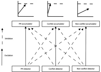
PMDC is an instance of the linear ballistic accumulator model (LBA; Brown & Heathcote, 2008), which formalizes decision making as a process of evidence accumulation among independent racers. The PMDC model uses three racing LBA accumulators; two correspond to the ongoing task responses and a third corresponds to the PM task response. Correct PM responses (PM hits) occur on PM trials when the PM accumulator reaches threshold before either of the ongoing task accumulators. PM misses occur when one of the ongoing task accumulators finishes before the PM accumulator. In Figure 1, we depict how this would apply in a relative trajectory judgment (conflict detection) task (e.g., deciding whether two aircraft are in conflict) with an additional PM requirement. There are three possible response alternatives, which correspond to indicating that the stimulus is a conflict, a non-conflict, or a PM target. Each response choice has its own accumulator that accrues evidence linearly (arrows in Figure 1), starting from points (uniformly distributed over the interval 0-A) representing random trial-to-trial biases. Evidence increases over time in a linear manner until the total in one accumulator reaches its response threshold (b). To avoid circularity, b is assumed to be set prior to the trial –
if it could be altered contingent on the identity of the stimulus there would be no need to make a
decision. The rate of accumulation – which varies normally from trial to trial with mean v and
standard deviation sv – corresponds to the strength of evidence for a choice, and it is determined
she attends to that information. The time for non-decision processes (e.g., stimulus encoding and
response selection, ter) is estimated by the difference between the observed RT and decision
[image:8.612.142.467.202.334.2]time (i.e., the time that evidence in the winning accumulator first equals the threshold).
Figure 1. An LBA model of a PM task with a concurrent conflict detection task. Evidence for each response is initially drawn from a uniform distribution on the interval [0, A]. Over time, evidence accumulates towards each response at rates drawn from independent normal distributions with mean v, and standard deviation sv. The first accumulator to reach its threshold, b, determines the overt response. We refer in our results to B, which is b – A, where B > 0 and so b > A. Total RT is determined by accumulation time plus non-decision time.
The aim of fitting the PMDC model is to measure the psychological quantities that
underlie performance, and to ascertain what those quantities suggest about resource allocation
and cognitive control. PMDC instantiates the proactive and reactive cognitive control
mechanisms specified by Braver’s (2012) dual-mechanisms theory and measures the overall
availability of resources, as well as the degree to which resources are shared between ongoing
task processing and PM task processing. We now review how PMDC instantiates these
mechanisms, and what has been found in the basic laboratory work with PMDC and other
evidence accumulation models.
Proactive control. Proactive control refers to processes used to "bias attention,
current theoretical (Bugg, McDaniel, & Einstein, 2013) and empirical PM research (e.g., Ball &
Brewer, 2018), proactive processes are deployed deliberately, in advance of the target stimulus
so that they are already active when the target stimulus is encountered. Proactive control should
thus be observable in differences between the latent processes underlying responses to (non-PM)
ongoing task items in PM blocks and control blocks. Under PMDC, participants proactively
control task demands by raising their thresholds in PM blocks, so that on PM trials the ongoing
task accumulators are less likely to complete before the PM accumulator, thereby reducing the
probability of a PM miss. This claim, originally made by the delay theory of PM cost (Heathcote
et al., 2015), follows from the fact that in evidence accumulation models, thresholds are the locus
of a priori strategies that drive mechanisms such as the speed-accuracy trade-off (Liu &
Watanabe, 2012) and response biases (Donkin, Brown & Heathcote, 2011; Mulder,
Wagenmakers, Ratcliff, Boekel & Forstmann, 2012).
indicating that ongoing task thresholds and PM thresholds are both important loci of proactive cognitive control strategies.
Reactive control. In contrast to proactive control, reactive control refers to automatic, stimulus-driven cognitive mechanisms that are deployed to influence responding "only as
needed, in a just-in-time manner" (Braver, 2012, p. 2). Reactive control mechanisms are
'bottom-up' processes and are assumed to operate automatically in response to inputs signalling the
critical event. As such, reactive control processes relevant to PM occur specifically on PM trials.
[image:10.612.129.483.321.574.2]PMDC’s reactive control mechanisms are depicted in Figure 2.
PMDC claims that as PM stimulus inputs are processed on PM trials, stimulus features
consistent with PM excite the PM accumulator, increasing accumulation speed, and inhibit other
accumulators (reactive inhibition), decreasing their accumulation speed. Thus, in addition to PM
accumulation being faster on PM trials than non-PM trials, accumulation towards ongoing task
decisions should be slower on PM trials than non-PM trials.1 The latter is the hallmark of
reactive control. In line with this, Strickland et al. (2018) found that ongoing task accumulation
rates were inhibited (reduced) on PM trials, and that this response competition brought about by
reactive control was critical to PM performance in basic PM laboratory paradigms. This
converges with other theoretical work (Bugg et al., 2013) and neurological data (McDaniel,
LaMontagne, Beck, Scullin, & Braver, 2013) implicating reactive control in PM, as well as
broader approaches to human error that contend that response inhibition is required for atypical
task responses to be able to compete for retrieval with task responses more strongly associated
with common environmental cues (Norman, 1981; Reason, 1990).
Capacity Sharing. PMDC measures capacity with the accumulation rate parameters, as have other models for measuring ongoing task capacity (Boywitt & Rummel, 2012; Horn et al.,
2011). Rates correspond to capacity because they estimate processing speed, which the majority
of attention theory assumes should vary in proportion to the attentional capacity available (e.g.,
1 Readers familiar with the intention superiority effect, in which ongoing task RTs are faster on PM target trials than
non-PM trials, may wonder whether reactive inhibition of rates on PM target trials is incompatible with the faster
RTs observed in the intention superiority literature (e.g., Marsh, Hicks, & Watson, 2002). However, on PM target trials, accumulators for the ongoing task responses must compete with a much faster PM response accumulator. Overt ongoing task responses on PM trials are therefore more likely to be fast errors that outpace the PM
Bundesen, 1990; Gobell, Tseng, & Sperling, 2004; Kahneman, 1973; Navon & Gopher, 1979; Wickens, 1980). Empirical work has also justified this connection, with rates converging with other measures of cognitive capacity (Donkin et al., 2014; Eidels, Donkin, Brown & Heathcote,
2010), and manipulations of capacity (e.g., adding a dual-task load) having the expected effects on rates (Castro, Strayer, Matzke & Heathcote, submitted; Logan et al., 2014).
The PMDC model allows for finer-grained analysis of capacity effects than do simple resource theories. For example, the model distinguishes the quantity of evidence accumulation from the quality of evidence accumulation. The quantity of accumulation is given by summing the rates for the matching and mismatching accumulators (‘matching’ refers to the accumulator for the response that matches the stimulus, i.e., the ‘correct’ response; ‘mismatching’ refers to the accumulator for the response that does not match the stimulus, i.e., the ‘incorrect’ response), whereas the quality of accumulation is given by the difference between the rates for the matching and mismatching accumulators. This distinction between the quantity and quality of
accumulation is not as apparent in the diffusion decision model (DDM; Ratcliff, 1978), which has been a commonly used measure of PM cost (e.g., Horn & Bayen, 2015).2
As reviewed, most PM theories assume that PM cost to non-PM trials results from reduced ongoing task capacity, the idea being that individuals need to orient attention towards monitoring for PM in case they are presented a PM item (e.g., Einstein & McDaniel, 2005; Smith, 2003). Testing this idea requires comparing ongoing task performance with and without PM demand (i.e., comparing accumulation rates to non-PM items in PM blocks with
2Ratcliff, Voskuilen, and Teodorescu (2018) have recently suggested that similar distinctions may be made with the
accumulation rates to non-PM items in control blocks). The majority of studies modeling PM costs have reported no change in either the quality or quantity of evidence accumulation to non-PM items across non-PM and control blocks, suggesting no change in the allocation or availability of resources as a result of PM (Ball & Aschenbrenner, 2017; Heathcote et al., 2015; Horn & Bayen, 2015; Strickland et al., 2017, 2018). In contrast, one recent study did find some evidence of
reduced processing quality under PM load (Anderson et al., 2018). However, this experiment did not counterbalance PM and control conditions, so it is possible that the evidence of reduced capacity was due to order effects rather than PM. Further contributing to the ambiguity of this effect, it only appeared in the diffusion decision model, and not in the LBA which provided a better fit to the data.
Prospective Memory in Complex Dynamic Tasks
To summarize the reviewed findings, it appears that in basic laboratory paradigms, individuals primarily manage PM demands by exerting cognitive control over ongoing task and PM processes, and that the capacity of the ongoing task is not affected by PM demands.
However, the previous data does not imply that PM monitoring never affects ongoing task resources. Indeed, a benchmark of resource theory is that tasks drawing on the same pool of resources may not interfere with each other unless the total demand for resources exceeds the
capacity limit of the cognitive system (Navon & Gopher, 1979; Norman & Bobrow, 1976). As
such, basic laboratory tasks may leave resources idle, meaning that there is sufficient capacity
available for monitoring in PM blocks without diverting resources from the ongoing task or increasing the amount of available resources (see Rummel, Smeekens, & Kane; 2017). This may render basic paradigms unable to detect capacity effects of PM that emerge when greater
Air traffic control is a prototypical example of a job in which people need to manage the demands of PM in a complex and dynamic environment (see Dismukes, 2010, 2012; Loft, 2014). Air traffic controllers are frequently faced with the requirement to remember to perform deferred actions. For example, a controller might need to remember to provide information to an aircraft when it passes a waypoint or reaches its top of descent. Alternatively, a controller might need to remember to change the route or level of one aircraft after giving a clearance to another aircraft, or to put an aircraft into a holding pattern. Controllers often do this when they are under
significant time pressure (Loft et al., 2007). For these reasons there is a growing body of both laboratory and field research examining PM using air traffic control tasks. These studies have
shown that PM produces numerous performance costs, including slower acceptance and hand-off
of aircraft, slower detection of conflicts between aircraft, and increased rates of missed conflicts
(Loft, Chapman, & Smith, 2016; Loft, Finnerty, & Remington, 2011; Loft, Pearcy, &
Remington, 2015; Loft, Smith, & Remington, 2013; Loft & Remington, 2010; Loft, Smith, &
Bhaskara, 2011; Loukopoulos, Dismukes, & Barshi, 2009). These costs observed by Loft and
colleagues, which affected both accuracy and RT, appear more consistent with resource sharing
than increased thresholds, inconsistent with the results from basic PM paradigms in which raised
ongoing task thresholds typically allow participants to maintain similar ongoing task accuracy in
control and PM blocks (e.g., Ball & Aschenbrenner, 2017; Heathcote et al., 2015; Horn &
Bayen, 2015; Strickland et al., 2017, 2018).
In the current study, we apply the PMDC model so that we can measure capacity and
control as has been done in the basic research. In our study, participants make decisions about
whether two aircraft will come into conflict at some point in the future. In some blocks of trials,
key instead of a conflict or non-conflict ongoing task response for aircraft with a callsign
containing two of the same letter (e.g., APA169, RTR451). Comparing model parameters
between control and PM blocks allows us to examine how PM affects attentional resources (e.g.,
capacity-sharing) and cognitive control mechanisms. To further test the role of capacity sharing
in PM cost, we introduce a further within-subjects manipulation of ongoing task demands: time pressure. This allows us to examine whether capacity for PM and ongoing processes trades off across different levels of time pressure, which is important because such trade-offs are a critical indicator of capacity sharing (Navon & Gopher, 1979). To impose time pressure on responses, we manipulated the number of items that needed to be sequentially responded to (trial load), and
the total time available to make that set of responses (trial duration). This was done to check
whether trial load and time available both induce quantitatively similar time pressure effects,
since this is not always the case in air traffic control or similar complex dynamic tasks (Loft et
al., 2007; also see Hendy, Liao, & Milgram, 1997; Palada, Neal, Tay, & Heathcote, 2018). We
now discuss testing the PMDC model as it would apply to the air traffic control task.
Testing Capacity and Cognitive Control
One question of interest is whether PMDC is capable of fitting the performance data from our conflict detection task. Evidence accumulation models have proved useful for understanding conflict detection in the past (Neal & Kwantes, 2009; Vuckovic, Kwantes, Humphreys, & Neal, 2014; Vuckovic, Kwantes, & Neal, 2013), accounting for accuracy and RT, and providing
sensible psychological interpretations of the effects of manipulations of bias and speed-accuracy
instructions. However, previous models required task-specific inputs such as relative speed and
angle of approach, and thus have limited generalizability beyond the specific scenarios on which
individual’s RT distributions and observed responses simultaneously. For the most part, evidence
accumulation models have only been fit in this way to short time scale decisions (typically < 1
second), but recent studies have revealed promise for fitting to longer time scale decisions. For
example, Lerche and Voss (2017) demonstrated good fits of the diffusion decision model to
decisions with mean RTs over 7 seconds. Further, they found that tests of selective influence
held, that is, manipulations affected rates where they were expected to (e.g., stimulus quality
increased rates), and thresholds where they were expected to (e.g., strategy influenced
thresholds). Palada et al. (2016; 2018) also found that evidence accumulation models (DDM and
LBA) could fit slow RTs, pass tests of selective influence, and measure various forms of
cognitive capacity, when fitting performance to a complex dynamic unmanned aerial vehicle
surveillance task. Thus, we have reasonable grounds to expect that PMDC may fit to our data.
Providing it can, the way in which it does so can give insight into the latent cognitive control and
resource allocation mechanisms underlying the data, as we discuss further below.
Proactive control. We expect that participants will use cognitive control to manage demands associated with time pressure, in line with previous modeling of the speed-accuracy
trade off (e.g., Dutilh, Wagenmakers, Visser, & van der Maas, 2011; Forstmann et al., 2011;
Usher, Olami, & McClelland, 2002). For example, participants may adjust their ongoing task
thresholds to avoid hitting trial deadlines under high pressure (i.e., when there is little time
available per decision), or to take advantage of lax trial deadlines under low pressure (i.e., when
there is more time available per decision; Ratcliff & Rouder, 1998). Raising thresholds allows
one to gather more evidence before responding, which results in slower but more accurate
decisions. Lowering thresholds allows one to spend less time gathering evidence and make faster
over response bias (i.e., prioritizing one response over another). For example, in air traffic
control, failing to detect a conflict has far greater safety implications than erroneously classifying
a non-conflict as a conflict. As such, expert controllers strategically shift bias towards making
conflict responses under time pressure to ensure aircraft remain separated (Loft, Bolland,
Humphreys & Neal, 2009). In terms of the model, response bias is reflected in differences in
thresholds between competing accumulators, whereby responding is biased in favour of the
accumulator with the lower threshold.
We also expect to replicate the consistent findings from basic paradigms that individuals
manage PM task demands by exerting proactive cognitive control over ongoing task thresholds
(e.g., Heathcote et al., 2015; Strickland et al., 2017, 2018). That is, we expect to find higher
ongoing task thresholds in PM blocks than in control blocks. Our relatively high PM frequency
(see further below) may encourage stronger proactive control of ongoing task thresholds than in
basic paradigms, as may the highly non-focal nature of the PM task. Further, if PM demands do
decrease ongoing task capacity (also discussed further below), caution may also increase with
PM to reduce ongoing task errors (as has been recently found with dual-task capacity costs;
Castro, Strayer, Matzke & Heathcote, submitted).
The demands associated with time pressure and PM load may interact, leading different
cognitive control strategies to trade off. For example, when time pressure is low, participants
have little reason not to increase their ongoing task thresholds in PM blocks, whereas when time
pressure is high, increasing ongoing task thresholds too much could lead to failing to perform
responses before the deadline (Palada et al., 2018). Thus, ongoing task thresholds in PM blocks
pressures. Participants may also lower PM thresholds with increased time pressure to ensure that
a PM response, if appropriate, is made before the response deadline.
Capacity Sharing. As with previous work, we examine how task demands affect the availability and allocation of resources by comparing ongoing task accumulation rates between different experimental conditions. We test for differences in resource availability in terms of the quantity (sum of matching and mismatching) of accumulation rates. Quantity reflects the total
amount of resources deployed by the cognitive system, which might increase and decrease to
meet task demands. For example, the quantity of available resources may increase as time
pressure increases. PM load may place demands on the cognitive system similar to time pressure,
and thus have similar effects on resource availability. In particular, quantity may increase in PM blocks if PM load increases the resources needed to perform the task, and perhaps also to
compensate for PM-induced proactive control over ongoing task thresholds, which makes it
difficult to respond before trial deadlines. Moreover, ongoing task and PM rates may trade-off
across different levels of time pressure (i.e., capacity may be shunted from PM to ongoing
processes as demands increase). Such a trade-off would demonstrate capacity sharing.
We also compare the quality of evidence accumulation (matching – mismatching accumulator ongoing task rates) across PM load and time pressure conditions. Palada et al. (2018) found that time pressure could cause a ‘redline’ to be crossed, after which performance
rapidly degraded. Imposing shorter trial deadlines led to reduced processing quality, which
participants attempted to compensate for by increasing their rate of information processing (i.e.,
quantity). This suggests that higher time pressure blocks should be more demanding than lower
ongoing task processing. Lower quality processing for ongoing task decisions under PM load would indicate that resources are being repurposed from the ongoing task to the PM task. Capacity effects may also occur because the PM cues (callsign) in our task are visually separate from the stimulus cues relevant to the ongoing conflict detection task (circular icons representing aircraft, speed indicator, relative distance of aircraft from the intersection), meaning that
detecting callsign cues will likely require participants to orient attention away from the visual location of the primary task, towards the PM cue.
In addition to our behavioural measures of quantity and quality, we include subjective
measures of effort, mental-, and temporal-demand (three subscales of the NASA-TLX; Hart &
Staveland, 1988). This will let us check whether participants’ subjective experiences of PM
demands and time pressure align with the resource availability and resource allocation
mechanisms in our model.
Reactive control. Trivially, we expect ‘reactive excitation’, in which PM accumulation rates are higher to PM items than non-PM items. In addition, previous applications of PMDC
have found inhibition of ongoing task accumulation rates to PM items. That is, accumulation
rates for conflict and non-conflict decisions should be lower for PM items, as compared with
non-PM items from PM blocks. Because reactive control only affects responses to ongoing task
stimuli when a PM item is present, it does not slow down overall responding very much, and so
decreasing reactive control with increased time pressure is not likely to much improve the
probability of meeting response deadlines. Thus, we do not have a strong reason to expect
Method
Participants
Of 49 participants two were excluded (see Results), with 47 participants remaining (31
females). Participants were recruited from the UWA undergraduate research pool and had no
prior experience with the air traffic control task. Ages ranged from 18 to 62 years (M = 25.19,
SD = 9.99). Participants completed one two-hour testing session. All procedures were approved
by the UWA Human Research Ethics Office.
Air Traffic Control Conflict Detection Task
The conflict detection task was designed by Fothergil, Loft and Neal (2009) in
consultation with subject matter experts using principles of representative design in order to
balance the competing demands of task fidelity, generality, and experimental control. The task
has been previously used to develop and test a performance theory and computational model of
expert conflict detection in air traffic control (Loft et al., 2009) and study PM (Loft, Smith, &
Bhaskara, 2011). As illustrated in Figure 3, each trial of the conflict detection task presented a single pair of aircraft cruising at identical altitudes and converging on a common intersection in a
fictitious en-route sector. The total area of the airspace was 180 nm (nautical miles) by 112.5 nm.
Each aircraft had a data block that displayed the callsign, the aircraft type, the flight level, and
the speed in knots (nautical miles per hour). Aircraft appeared within a circular air traffic control
sector with a neutral grey background and flew straight paths (indicated by black lines) which
converged at a 90-degree angle in the centre of the display. Aircraft position was updated every
20 ms. Participants had no control over the flight levels, velocities, or headings of the aircraft.
on whether the aircraft would violate a 5 nm minimum separation distance at some point during
their flight. On some trials one of the two aircraft would also contain a PM target feature which
required execution of a PM response instead of the conflict or non-conflict ongoing task
response. Within each trial, pairs of aircraft were presented sequentially; each pair disappearing
from the screen once a response was made. As shown in Figure 3, the display included a
countdown timer indicating the seconds remaining in each trial. Trials ended when the timer
reached zero, after which any remaining aircraft not responded to would disappear and be
recorded as non-responses. A 10 nm by 20 nm (approximately 2 cm by 4 cm on screen) scale
marker, used as a reference for judging relative aircraft distance, was fixed on the left side of the
display. Each aircraft had a probe vector line which showed the aircraft's heading and predicted
[image:21.612.73.536.396.657.2]position one minute into the future.
Experimental Stimuli and Design
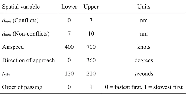
Table 1 specifies the range of values for the features of aircraft pairs and the distribution
they were drawn from. The angle of approach between aircraft was fixed at 90 degrees to avoid
interactions between angle and perceived conflict status (e.g., Loft et al, 2009; Vuckovic et al,
2013). The flight level for all aircraft was fixed at 37,000 feet. To create the different conflict
and non-conflict stimuli, each aircraft pair was assigned a miss distance (dmin: the distance
between the aircraft at their point of closest approach) either less than or greater than the 5 nm
separation standard. For conflict stimuli, dmin values were drawn from the uniform distribution
[0,3] nm. For non-conflict stimuli, dmin values were drawn from the uniform distribution [7,10]
nm. Because our primary interest here was in stable conflict detection performance, free from
learning effects, we allowed other aircraft features to vary randomly. These features were speed,
Table 1
Range of spatial variables of aircraft stimuli
Spatial variable Lower Upper Units
dmin (Conflicts) 0 3 nm
dmin (Non-conflicts) 7 10 nm
Airspeed 400 700 knots
Direction of approach 0 360 degrees
tmin 120 210 seconds
Order of passing 0 1 0 = fastest first, 1 = slowest first
Aircraft with callsigns containing two of the same letter (e.g., APA169, RTR451) were
PM targets, thereby emulating the general task demand that operators monitoring
perceptually-demanding displays can face to remember to perform a deferred task action in the future when
they observe a particular event (Loft, 2014). The PM target is non-focal to conflict detection
(Einstein & McDaniel, 2005), meaning that the evidence required to make PM decisions (i.e.,
assess aircraft callsign) is not required to make ongoing task conflict/non-conflict decisions (e.g.,
which requires assessing airspeed, relative distance, and position). On PM target trials only one
of the aircraft on screen ever contained a PM target, never both. Participants were instructed to
respond to PM targets by pressing an alternate PM key (e.g., ‘j’ or ‘d’) instead of the typical
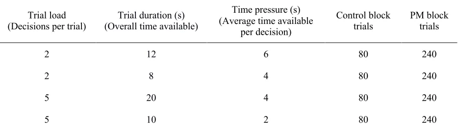
As illustrated in Table 2, participants performed four sets of trials, each containing a
block of control trials and a block of PM trials. Block order (control- or PM-first) was
counterbalanced between participants. In control blocks, participants were presented with a
randomized sequence of 80 aircraft pairs (40 conflict and 40 non-conflict), with no PM targets.
In PM blocks, participants were presented with a randomized sequence of 240 aircraft pairs (120
conflict and 120 non-conflict). Of these, a random 48 (24 conflict and 24 non-conflict) contained
[image:24.612.74.541.347.480.2]a PM target. Thus 20% (48/240) of PM block stimuli were PM targets.
Table 2
Details of experimental blocks with number of control and PM stimuli presented
Trial load
(Decisions per trial) (Overall time available) Trial duration (s)
Time pressure (s) (Average time available
per decision)
Control block
trials PM block trials
2 12 6 80 240
2 8 4 80 240
5 20 4 80 240
5 10 2 80 240
To create time pressure (average available time per conflict detection decision), we
manipulated trial load (decisions per trial) and trial duration (overall time available to respond to
all decisions within a trial). Each trial had a load of either 2 or 5 (i.e., 2 or 5 aircraft pairs
presented) with an associated trial duration (see Table 2). This resulted in 4 unique trial-load by
trial-duration combinations; one with 6s per decision, two blocks with 4s per decision and one
block with 2s per decision. Presentation order was counterbalanced across participants. We
intentionally did not orthogonally cross trial load with trial duration. This was done to ensure
becoming impossibly difficult. Participants were informed of the trial load and trial duration
prior to each block, giving them opportunity to adjust their strategies accordingly.
Procedure
Our primary goal when designing this experiment was to reliably model both ongoing
task and PM responses in a more complex and dynamic task than is typically used in PM
research. To this end, our task deviated slightly from traditional PM paradigms. Most PM studies
conducted using the Einstein and McDaniel (1990) paradigm present only a small number of PM
targets, and as such they do not produce enough data to reliably constrain a model of PM
processes. Moreover, because the conflict detection task involves much slower RTs than typical
laboratory paradigms, we were limited in the number of trials we could present to participants in
a single 2-hour testing session. As such, we modified the paradigm by increasing the ratio of PM
target trials to ongoing task trials to 1 in 5 trials (i.e., 20% of PM block stimuli were PM targets).
This gives us more PM trials, which serve to reliably constrain our model, and increase the
accuracy and precision of model fitting.
Each testing session consisted of a training phase and a test phase with total duration of 2
hours. During training participants received verbal task instructions, watched an on-screen
demonstration, and completed a block of 40 training trials which included feedback after each
response. PM targets were not included in training. During the experimental phase participants
completed eight blocks of experimental trials, which did not include feedback.
Participants responded to each aircraft pair by pressing the conflict key or the
non-conflict key. Participants were told that each aircraft pair would be presented sequentially (i.e.,
only two aircraft would appear on screen at a time), that all aircraft would be moving towards
number of spatial properties of the aircraft would vary from trial to trial, including their starting
distance from the central crossing point, relative speed, and miss distance. Before each block of
trials, participants saw visual instructions reminding them of the trial load and trial duration for
that block. Depending on the block, participants received either control or PM instructions.
Before control blocks, participants were instructed that they only needed to make conflict and
non-conflict responses. Before PM blocks, participants were instructed to press a PM response
key instead of the conflict or non-conflict keys when they detected a PM target. Participants then
completed a short distractor task and saw a final reminder to respond as quickly and accurately
as possible before commencing the block.
Four response key assignments were counterbalanced across participants; 1) s = conflict,
d = conflict, j = PM, 2) d = conflict, s = conflict, j = PM, 3) k = conflict, j =
non-conflict, d = PM, and 4) j = non-conflict, k = non-non-conflict, d = PM. So that we could assume equal
motor response time in our modeling (see Voss, Voss, & Klauer, 2010), participants were
instructed to rest their fingers on their particular response key combination throughout the task.
A screen with the text 'Press [Space] to continue' preceded each trial, and each trial began once
the space-bar was pressed.
Trials ended when either all aircraft pairs had been responded to (2 pairs during blocks of
low-load trials; 5 pairs during blocks of high-load trials) or when the response deadline expired
(i.e., the timer reached zero). Aircraft pairs not responded to within the response deadline were
recorded as non-responses. Participants were informed that conflict detection misses (responding
no further feedback was given concerning task performance. Participants took self-paced breaks
between each block of trials and were also permitted short breaks at any point between trials if
required. Subjective task demand after each block was assessed using the NASA Task Load
Index (Hart & Staveland, 1988). The NASA-TLX comprises six items: three that tap task
demand (i.e., mental, physical, and temporal demand) and three which tap the individual's
subjective perception of exertion and task performance (i.e., performance, effort, and
frustration). Each item is rated on a 21-point numerical scale, with higher scores being indicative
of higher workload.
Results
Conventional statistical analyses are reported first in order to check whether our
experimental manipulations had the expected effects on RT, accuracy, and non-response (miss)
rate. Data from two participants was excluded; one participant who failed to complete all
experimental blocks and one who made no PM responses at all. We excluded trials with outlying
RTs, defined as less than 0.2s or 3 times the inter-quartile range / 1.349 (a robust measure of
standard deviation) above the mean (1.52% of responses overall). Outliers were censored
separately for each different time pressure condition. Overall, 6.3% of the data comprised
non-response misses, ranging from 2.5% in the lowest time pressure condition, to 14.8% in the
highest. Two kinds of extremely rare responses – incorrect ongoing task responses to PM items
(1.5% of PM block responses), and PM responses to control-block ongoing-task stimuli (0.4% of
all responses) – are not analysed further. The conventional statistical analyses compare mean
accuracy and RT by stimulus type (conflict, non-conflict, PM) PM block (control, PM) and time
compared separately for each level of trial load. That is, at low trial load (2 decisions per trial)
we compare time pressures of 6 and 4 seconds per decision, and at high trial load (5 decisions
per trial) we compare time pressures of 4 and 2 seconds per decision.
In our significance testing for accuracy effects we used generalized linear mixed models
with a probit link function. In our significance testing for mean correct RTs we used general
linear mixed models.3 Analyses were conducted using the R package lme4 (Bates, Machler,
Bolker, & Walker, 2015), and significance assessed with Wald's chi-square tests (Fox &
Weisberg, 2011), using an alpha level of 0.05. Post hoc tests applied Bonferroni’s correction for
alpha inflation. The results of our analyses are tabulated in the supplementary materials (Tables
S1-S4). All standard errors reported in text and displayed in graphs were calculated using the
within-subject bias-corrected method (Morey, 2008).
Conflict Detection (Non-PM) Trials
Accuracy was lower for conflicts (67.4%) compared with non-conflicts (80.6%) and
slightly lower under PM load compared with control (Control: M = 74.9%, SE = 3.2%; PM: M =
73.1%, SE = 3.3%). Conflict detection accuracy decreased as time pressure increased, under both
low trial-load (6s: M = 76.9%, SE = 2.7%; 4s: M = 74.8%, SE = 2.7%) t = 2.60, df = 46, p = .012,
3We used two methods of analysis to check that the inferences derived from each method agreed. For our accuracy
Cohen’s d = 0.38, and high trial-load conditions (4s: M = 75.7%, SE = 2.5%; 2s: M = 68.6%, SE
= 2.6%) t = 7.82, df = 46, p < .001, d = 1.14. Conflict detection accuracy was not significantly
affected by trial load when comparing cells with equal time pressure. There was a significant
interaction between PM block and time pressure on accuracy, such that the cost to PM block
accuracy was greatest when trial load and time pressure were also high (Control: M = 70.9%, SE
= 2.1%; PM: M = 66.3%, SE = 2.5%), t = 4.25, df = 46, p < .001, d = 0.62.
Mean RT was slower for conflicts (3.09s) compared with non-conflicts (2.75s), slower
for errors (2.99s) compared with correct responses (2.91s), and slower during PM blocks than
control blocks (Control: M = 2.65s, SE = 0.17s; PM: M = 3.07s, SE = 0.17s). Mean RTs were
significantly faster under higher time pressure for both low trial-load (6s: M = 3.65s, SE = 0.14s;
4s: M = 2.80s, SE = 0.08s) t = 7.14, df = 46, p < .001, d = 1.04, and high trial-load conditions (4s:
M = 2.95s, SE = 0.10s; 2s: M = 2.04s, SE = 0.07s) t = 12.26, df = 46, p < .001, d = 1.79. Mean
RTs were also slower under high trial load compared with low trial load when comparing cells
with equal time pressure, t = -2.17, df = 46, p = .035, d = 0.32, although this effect was small.
There was no significant interaction between PM block and time pressure on mean RT.
To summarize, the addition of PM load resulted in slower (Mean Difference = 0.42s) and
slightly less accurate (Mean Difference = 1.8%) ongoing conflict detection task performance,
while increased time pressure led to faster (Mean Difference = 0.88s) but less accurate (Mean
Difference = 4.6%) ongoing conflict detection task performance.
PM Trials
PM responses were scored correct if the participant made a PM response instead of an
ongoing task (conflict/non-conflict) response on PM target trials. PM accuracy decreased as time
2.1%) t = 3.19, df = 46, p = .003, d = 0.47, and high trial-load conditions (4s: M = 73.8%, SE =
1.9%; 2s: M = 58.6%, SE = 2.7%) t = 4.94, df = 46, p < .001, d = 0.72. PM accuracy was not
significantly affected by trial load when comparing cells with equal time pressure. PM accuracy
was weakly positively correlated with ongoing task accuracy (r = .21, p < .001).4
Mean RT was slower for PM errors (2.73s) compared with correct PM responses (1.77s)
(in PM blocks). Mean RT for correct PM responses was significantly faster at higher levels of
time pressure during both low trial-load (6s: M = 2.00s, SE = 0.05s; 4s: M = 1.78s, SE = 0.05s) t
= 3.96, df = 43, p < .001, d = 0.60, and high trial-load conditions (4s: M = 1.89s, SE = 0.05s; 2s:
M = 1.58s, SE = 0.05s) t = 6.40, df = 44, p < .001, d = 0.95. PM RTs were slower under high trial
load compared with low trial load when comparing cells with equal time pressure, t = -2.13, df =
43, p = .039, d = 0.32, although this was a relatively small effect. There were no significant
differences in PM accuracy or PM RT between conflict PM targets and non-conflict PM targets. PM false alarms (i.e., PM responses to non-PM stimuli in PM blocks) occurred on 0.56% of PM
block trials with a mean RT of 2.45s. Mean PM RT was moderately positively correlated with
mean ongoing task RT (r = .48, p < .001). To summarize, as with the ongoing task, increased
time pressure led to faster (Mean Difference = 0.27s) but less accurate PM performance (Mean
Difference = 11.4%).
4The correlation between ongoing task and PM accuracy is consistent with the strong role of proactive control
Non-responses
We ran a linear mixed effects model (Table S6 in the supplementary materials) to
examine the effects of PM block and time pressure on non-response (miss) proportions
(non-responses included non-(non-responses to PM and ongoing task stimuli). Non-(non-responses were slightly
more frequent in PM blocks compared with control (Control: M = 5.8%, SE = 1.6%; PM: M =
5.9%, SE = 1.8%), and became more frequent as time pressure increased during both low
trial-load (6s: M = 2.2%, SE = 1.0%; 4s: M = 4.4%, SE = 0.9%) t = 2.71, df = 46, p = .009, d = 0.4,
and high trial-load conditions (4s: M = 3.0%, SE = 0.8%; 2s: M = 13.8%, SE = 1.7%) t = 6.29, df
= 46, p < .001, d = 0.92. The proportion of non-responses was not significantly affected by trial
load when comparing cells with equal time pressure, t = -1.89, df = 46, p = .07, d = 0.28. There
was a significant interaction between PM block and time pressure on non-responses, such that
the increase in non-responses from control to PM blocks was greatest when trial load and time
pressure were both high (Control: M = 12.0%, SE = 1.4%; PM: M = 14.7%, SE = 1.7%), t = 2.17,
df = 46, p = .04, d = 0.32. This suggests a drawback of using the proactive control strategy under high time pressure. That is, higher ongoing task thresholds caused decisions to exceed the trial
deadline more often, resulting in more non-responses to ongoing task stimuli.
NASA-TLX Demand Ratings
We ran a linear mixed effects model (Tables S7-S9 in the supplementary materials) to
examine the effects of PM block and time pressure on self-report effort, mental-, and
temporal-demand ratings. Effort was significantly higher in PM blocks than control blocks (Control: M =
12.08, SE = 0.68; PM: M = 13.50, SE = 0.71). Effort was also higher in high time pressure blocks
during both low trial-load (6s: M = 11.38, SE = 0.57; 4s: M = 13.13, SE = 0.52) t = 2.80, df = 46,
0.46) t = 6.93, df = 46, p < .001, d = 1.01. Effort was lower during high trial load compared with
low trial load when comparing cells with equal time pressure, t = 2.93, df = 46, p = .005, d =
0.43. There was no interaction between PM block and time pressure on effort.
Similarly, mental demand was significantly higher in PM blocks than control blocks
(Control: M = 12.31, SE = 0.57; PM: M = 14.60, SE = 0.58). Mental demand was also higher at
higher levels of time pressure during both low trial-load (6s: M = 12.47, SE = 0.48; 4s: M =
13.41, SE = 0.39) t = 2.16, df = 46, p = .036, d = 0.31, and high trial-load conditions (4s: M =
12.35, SE = 0.44; 2s: M = 15.60, SE = 0.51) t = 6.55, df = 46, p < .001, d = 0.96. Mental demand
was lower during high trial load compared with low trial load when comparing cells with equal
time pressure, t = 2.78, df = 46, p = .008, d = 0.41. There was no interaction between PM block
and time pressure on mental demand.
Temporal demand was significantly higher in PM blocks than control blocks (Control: M
= 11.75, SE = 0.82; PM: M = 13.37, SE = 0.97). Temporal demand was also higher at higher
levels of time pressure during both low trial-load (6s: M = 9.48, SE = 0.56; 4s: M = 13.15, SE =
0.56) t = 6.02, df = 46, p = < .001, d = 0.88, and high trial-load conditions (4s: M = 10.61, SE =
0.61; 2s: M = 17.01, SE = 0.54) t = 9.80, df = 46, p < .001, d = 1.43. Temporal demand was
lower during high trial load compared with low trial load when comparing cells with equal time
pressure, t = 3.58, df = 46, p = .001, d = 0.52. There was no interaction between PM block and
findings give us confidence that our PM and time pressure manipulations were effective at
inducing different levels of subjective task demand.5
Model Analysis
Our design includes several factors over which model parameters can vary, including
latent response (i.e., conflict, non-conflict, and PM accumulators), and three manifest factors,
stimulus type, time pressure/trial load, and PM demand. The latent response factor refers to the
accumulators that can lead to each response (conflict, non-conflict, PM). The latent response
factor corresponds to the accumulators, and not the response that was actually observed; the
observed response is predicted by, not included in, the model. The stimulus type factor had four
levels: non-PM conflict, non-PM non-conflict, PM conflict, and PM non-conflict. Since the
trial-load (2 versus 5 decisions per trial) and task-duration factors were not crossed orthogonally, they
were captured by a four-level composite factor created by manipulating trial load and trial duration with the following levels: 6s per decision (2 decisions per trial), 4s per decision (2 decisions per trial), 4s per decision (5 decisions per trial), 2s per decision (5 decisions per trial). The PM demand factor had two levels: control (i.e., no PM demand) and PM.
To reduce model complexity, we applied several theoretically sensible a priori
constraints on which factors each parameter could vary. First, we estimated one common A
parameter for all accumulators and conditions, as is common practice in LBA modeling. Second,
5The correlations between the subjective effort ratings and various model parameters (e.g., rate quality and
we allowed the sv parameter to vary by stimulus and accumulator factors but not over PM block
or time pressure. This is more flexible than most previous LBA modeling, which typically only
allows sv to vary as a function of whether the latent accumulator matches or does not match the
stimulus6 (but see Heathcote & Love, 2012; Osth, Bora, Dennis, & Heathcote, 2017; Strickland
et al., 2018, for exceptions). We used this more flexible approach because in our model there are
two types of 'correct' response for PM trials (i.e., correct PM and correct ongoing task decision).
We fixed the sv parameter for PM false alarms (i.e., 'PM' responses to non-PM stimuli) at 0.5,
because one accumulator parameter must be fixed to an arbitrary value as a scaling parameter
(Donkin, Brown, & Heathcote, 2009).
Third, we estimated only one non-decision time (ter) parameter for each participant. This
was done because our design minimized any potential differences in the motor movement
required to make each response (i.e., participants kept their fingers positioned above the response
key which were all located on one keyboard row). In addition, previous research has shown
non-decision time does not play a role in PM cost for the LBA (e.g., Anderson et al., 2018; Heathcote
et al., 2015; Strickland et al., 2017, 2018). Finally, due to very low numbers of PM false alarms
(PM responses to non-PM stimuli in PM blocks) we pooled estimates of both accumulation rate
and variance (v and sv) across all experiment factors to give one PM false alarm rate and one
corresponding sv parameter (which was used as a fixed scaling parameter as mentioned above).
These a priori restrictions resulted in an 89 parameter most flexible 'top' model with one A, one
6We also fit a version of the model with only one sv parameter. This model had fewer parameters (75), produced
ter, 20 B, 57 v, and 10 sv parameters. We compared this flexible top model against several
simpler, more constrained variants as outlined in the Model Selection section below.
Sampling
We estimated model parameters using the DMC software (Heathcote, et al., 2018) to
perform Bayesian estimation, which results in probability distributions that reflect the certainty
about parameter values. Although in principle we could have fit a hierarchical model to estimate
the common population distributions of each parameter, we estimated parameters separately for each participant for several reasons. First, since this is the first time that such a model has been fit to this kind of task, we did not have adequate knowledge of the appropriate form of the
population-level distributions. Because inappropriate population-level assumptions can introduce inappropriate shrinkage effects in hierarchical models, fitting to individual participants avoids such issues. Second, because of the large number of participants in our sample and the
complexity of our models, hierarchical methods proved too computationally expensive to fit (estimated at several months of multi-core server time per fit).
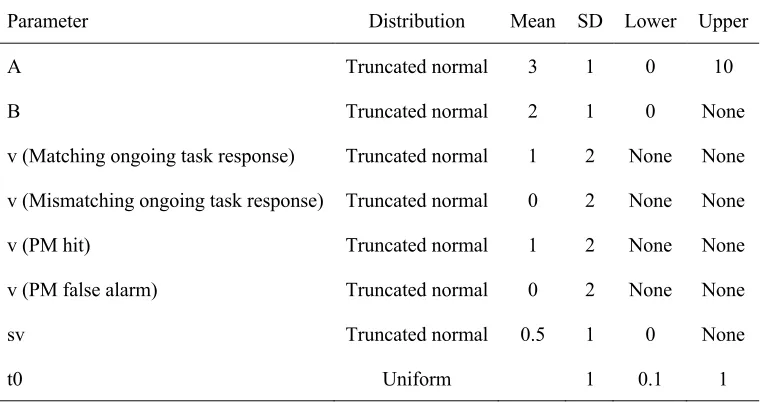
Bayesian analysis requires that the researcher specify prior beliefs about the probabilities
of parameters and the form of their distributions before observing the data. However, because of
our large sample sizes and use of inference based on posterior probability distributions, the
influence of our particular choice of priors on the final parameter estimates was negligible. Since
these analysis techniques have not been used on a dynamic complex task, we did not have strong
reasons to prefer one particular set of priors over others. We used relatively non-informative
priors similar to Strickland et al. (2018), but with higher threshold priors to account for our
slower mean RTs (Table 3). All prior values were the same over control and PM blocks and the
Posterior parameter distributions were estimated using the differential evolution
Markov-chain Monte-Carlo (MCMC) algorithm (Turner, Sederberg, Brown, & Steyvers, 2013).
DE-MCMC is more adept than conventional samplers at handling the high parameter correlations
common to accumulate-to-threshold models. The number of chains was three times the number
of parameters (e.g., for an 84-parameter model there were 252 chains per parameter). Chains
were thinned by 20, meaning that one iteration in every 20 was kept. Sampling continued for
each participant until a small Gelman's (2014) multivariate potential scale reduction factor (<1.1)
indicated convergence, stationarity, and mixing. Convergence, stationarity, and mixing were
verified by visual inspection. We retained the same number of samples for each participant: each
of the 252 chains was 120 iterations long, producing 30,240 samples of each parameter's
[image:36.612.74.455.456.657.2]posterior distribution for each participant.
Table 3
Prior distributions
Parameter Distribution Mean SD Lower Upper
A Truncated normal 3 1 0 10
B Truncated normal 2 1 0 None
v (Matching ongoing task response) Truncated normal 1 2 None None
v (Mismatching ongoing task response) Truncated normal 0 2 None None
v (PM hit) Truncated normal 1 2 None None
v (PM false alarm) Truncated normal 0 2 None None
sv Truncated normal 0.5 1 0 None
Model Results
Model Fits: Accuracy and RT
To evaluate fit, we sampled 100 posterior predictions for each participant and then
averaged over participants. The model provided good fits to both ongoing task and PM accuracy
(Figures S1-S2 in the supplementary materials) and gave a good account of the entire distribution
of response times (Figures S3-S5). The model provided a close fit to the differences in manifest
accuracy and RT observed across PM and control blocks and across different time pressures.
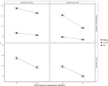
Model Fits: Non-response Proportions
As noted earlier, our data contained significant differences in non-response proportions
between time pressure blocks. Because non-responses were not included in model fitting, this
gave us an opportunity to test PMDC’s consistency with unseen data. That is, we assessed how
well the model could make out-of-sample predictions of empirical non-response proportions. In
order to do this, we simulated data out of the selected model (see Table 4) and matched the order of the simulated stimuli and responses to the actual presentation order experienced by each participant (this was done to ensure that the simulated trials had the same stimulus-response content as the empirical trials). Whenever the cumulative sum of simulated RTs within a trial exceeded that trial's deadline, a non-response was predicted. Using this method, 100 posterior predictions for non-response proportions were sampled for each participant and predictions were then averaged over all participants. We then compared the predicted non-responses with
proportions closely match the empirical non-response proportions, demonstrating the ability of the model to predict data out of sample.
Figure 4. Model fits to non-response proportions by PM block and time pressure. Data effects are represented by unfilled circles. Model predictions are represented by filled circles with 95% credible intervals.
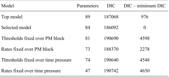
Model Selection
We applied model selection to assess whether we could justify constraining model
parameters over blocked experimental conditions (e.g., PM block, time pressure) to obtain a
simpler model with fewer parameters. To select between models, we used the Deviance
Information Criterion (DIC; Spiegelhalter, Best, Carlin, & Van Der Linde, 2002), a measure
models with smaller DIC values are to be preferred. Table 4 shows each model we compared, its
[image:39.612.75.421.234.393.2]number of parameters, and DIC value.
Table 4
DIC model selection. Lower DIC indicates more preference for the model.
Model Parameters DIC DIC – minimum DIC
Top model 89 187068 976
Selected model 84 186092 0
Thresholds fixed over PM block 81 190690 4598
Rates fixed over PM block 73 188370 2278
Thresholds fixed over time pressure 74 190640 4548
Rates fixed over time pressure 47 190742 4650
Starting with the fully flexible top model, we built several simpler variants by
systematically constraining ongoing task threshold and ongoing task rate parameters over PM
and time pressure. This allowed us to assess whether it was necessary to vary ongoing task
thresholds and/or rates to account for the observed PM demand and time pressure effects (i.e., to
test whether proactive control and/or capacity-sharing were necessary mechanisms in the model).
PM thresholds and rates were left free. We compared the following four constrained models to
the top model: a model in which rates could vary across PM and control blocks but thresholds
could not; a model in which thresholds could vary across PM and control blocks but rates could
not; a model in which rates could vary by time pressure but thresholds could not; and a model in
As Table 4 shows, in each case the simpler model was rejected in favour of the fully
flexible top model, suggesting that it is necessary to allow both ongoing task threshold and
ongoing task rate parameters to vary over PM and time pressure (i.e., both parameters are
influenced by PM and time pressure manipulations and are important in explaining the observed
data).
Finally, we tested an additional model (the selected model) that, like the top model,
allowed both rates and thresholds to vary over both PM and time pressure but included a slight
simplification: the PM rate parameter was constrained to not vary over stimulus type (i.e., PM
conflicts and PM non-conflicts had the same rate). This simplification makes theoretical sense,
since the evidence used to make a PM decision was independent of the evidence used to make
either conflict or non-conflict ongoing task decisions. This slightly simpler model produced the
smallest DIC value and was thus selected as our preferred model for further analysis.
The results of model selection suggest that both rates and thresholds have some role in
explaining ongoing task and PM accuracy and RT under different levels of PM demand and time
pressure. However, we wanted to further break down how each part of the model contributes to
observed accuracy and RT. To this end, in the next section we test the direction and magnitude
of differences between conditions in the parameters of the selected model. Testing the direction
of effects is important because it allows us to identify how cognitive control and resource
allocation mechanisms contribute to performance, and thus to distinguish between competing
theories of PM and task demand, whose predictions are also directional (e.g., capacity-sharing
theories predict lower rates in PM blocks than in control blocks). Testing the magnitude of
(such as costs to accuracy and RT) and which are most affected by a given experimental
manipulation (such as time pressure).
Model Summary
To summarize the parameters of the group of participants, we created a subject-average
posterior distribution. This was obtained by computing the mean of each posterior sample over
all participants for each parameter. Our primary theoretical interest was in threshold and rate
parameters for the ongoing and PM tasks, which we explore in detail in the following sections.
The other parameters all had reasonable values. The non-decision time mean of the
subject-average posterior distribution was 0.35 seconds (posterior SD = 0.01 seconds). The A posterior
mean was 3.34 (posterior SD = 0.04). The sv posterior means and SDs are summarized in Table
5. Consistent with other LBA studies, sv parameters for the ongoing task are lower for matching
response accumulators compared with mismatching response accumulators when it was a
non-PM stimulus. For non-PM stimuli there was little difference in sv between accumulators. The
[image:41.612.74.406.539.653.2]accumulation rate for PM false alarms was -1.30 (posterior SD = 0.05).
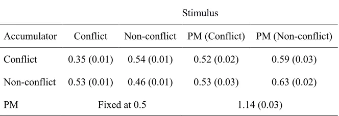
Table 5
Mean (SD) of the average posterior sv parameter samples
Stimulus
Accumulator Conflict Non-conflict PM (Conflict) PM (Non-conflict)
Conflict 0.35 (0.01) 0.54 (0.01) 0.52 (0.02) 0.59 (0.03)
Non-conflict 0.53 (0.01) 0.46 (0.01) 0.53 (0.03) 0.63 (0.02)
The direction and magnitude of differences in ongoing and PM threshold and rate
parameters for the selected model across conditions were examined to assess how well they
correspond to the theoretical predictions of capacity sharing, proactive control, reactive control,
and arousal/availability. We calculated posterior distributions of the differences between
experimental conditions. For example, to test the difference between ongoing task response
thresholds in control and PM blocks (i.e., testing the proactive control account of PM costs), we
subtracted the control block threshold from the PM block threshold for every posterior sample,
thus obtaining the posterior probability distribution of the difference between control and PM
thresholds. Differences were calculated independently for each participant before being averaged
across participants to create a subject-averaged posterior difference distribution. For each
subject-averaged difference distribution we report a Bayesian p-value (Klauer, 2010), which
indicates the one-tailed probability that the effect does not run in the most sampled direction.
Due to the large number of trials per participant in our design, almost all our observed
parameter differences have p-values very close to zero, indicating a very high probability that an
effect was present. However, some of our parameter differences were much larger in magnitude
than others. As such, we illustrate the magnitude of the effect by reporting the standardized
difference between parameters (i.e., M / SD of the posterior difference distribution). Because our
posterior parameter distributions are approximately normal, this standardized statistic can be
interpreted in a similar way to a score. We therefore refer to this statistic as Z from here on.
Z-score effect sizes and p-values for parameter comparisons are shown in Tables S10-S19 in the
![Figure 1. An LBA model of a PM task with a concurrent conflict detection task. Evidence for each response is initially drawn from a uniform distribution on the interval [0, A]](https://thumb-us.123doks.com/thumbv2/123dok_us/8388730.322904/8.612.142.467.202.334/concurrent-conflict-detection-evidence-response-initially-distribution-interval.webp)