Free surface interaction of a ‘T-foil’ hydrofoil
by
Alexander John Edwin Ashworth Briggs, MSc
National Centre for Maritime Engineering and Hydrodynamics
Australian Maritime College
Submitted in fulfilment of the requirements for the degree of
Doctor of Philosophy
This thesis contains no material which has been accepted for a degree or diploma by the University or any other institution, except by way of background information and duly acknowledged in the thesis, and to the best of my knowledge and belief no material previously published or written by another person, except where due acknowledgement is made in the text of the thesis, nor does the thesis contain any material that infringes copyright.
This thesis may be made available for loan and limited copying and communication in accordance with the Copyright Act 1968.
Signed: ____________________________________________
The publishers of the papers comprising Chapters 3, 4 and 5 hold the copyright for that content, and access to the material should be sought from the respective journals. The remaining unpublished content of the thesis may be made available for loan, limited copying and communication in accordance with the Copyright Act 1968.
Statement of co-authorship
The following people contributed to the manuscripts included as part of this thesis: Alexander Ashworth Briggs (Candidate)
Associate Professor Jonathan Binns (Author 1) Dr Jonathan Duffy (Author 2)
Dr Alan Fleming (Author 3)
I would like to thank the following people for their support in this endeavour.
My supervisors: Associate Professor Jonathan Binns for getting me to the AMC and your enthusiasm to make things happen, Dr Jonathan Duffy, your ability to listen, distil the issues and provoke thought helped me enormously, and Dr Alan Fleming for your outwardly untiring patience with a Python newbie and guidance with the setup of the Particle Image Velocimetry system. Dr Roberto Ojeda Rabanal for your early supervision, unfortunately the project went in a different direction.
Associate Professor Paul Brandner and Dr Bryce Pearce, for taking the time out of your busy schedules to discuss fluid dynamics, give general feedback on experimental results, and for your reading recommendations. Not forgetting Professor Michael Woodward, for sharing your ‘fractal’ approach and advising on experimental uncertainty.
The academics and staff of the towing tank, with a particular thank you to Associate Professor Gregor MacFarlane, for making the towing tank, and his key personnel, Tim Lilienthal and Liam Honeychurch, available to assist with the experimental setups. Thank you also Michael Underhill, Jock Ferguson and Darren Young, for without your assistance with the manufacture of experimental components, and the sharing of your departmental brand of humour, all would have been lost.
My peers Chris Polis, Philip Marsh, Alexander Conway, and Zhi Q Leong with whom sailing, beer, food and stimulating conversation have been shared.
Thank you my wonderful wife, for being your delightful self, my partner in crime, brilliant proof reader and the best thing that ever happened to me.
My parents-in-law, Christopher and Victoria Preston for your tireless enthusiasm, support and being equally ‘difficult’.
To my father, for showing me that
This thesis presents an investigation of the flow field around the tip vortex of a t-foil hydrofoil. The objective of the investigation was to gain understanding of the mechanisms surrounding the inception of tip vortex ventilation of t-foil hydrofoils which will inform the evolution of the next generation of t-foil hydrofoil design for both commercial passenger and high performance sail craft.
Qualitatively – Observations from images taken during high speed towing tank testing at velocities between 2 to 12 ms-1 were compared and estimations made of the wake age, and
the submergence, at which tip vortex filament cavitation and tip vortex ventilation may occur in a controlled environment. Quantitatively – Particle Image Velocimetry (PIV) velocity fields were obtained experimentally for a vertically mounted flat plate at angle of incidence and a NACA 0012 t-foil hydrofoil at an angle of attack (AoA) of 8o, with a submergence to
chord ratio (h/c) of between 0.11 and 1.70 and at streamwise distance to chord length ratio or wake age (x/c) of between 0 and 5. The flow fields were compared using the metrics of circulation, peak tangential velocity, vorticity and velocity profiles of the components of the planar cross velocity.
A methodology was developed for tracking the location of the wandering vortex core and the experimental and numerical results compared. At high angle of attack the numerical results identified that vortex shedding from the leading edge separation of the test geometry is a possible contributory factor to the vortex wandering phenomena. The vortex centre and the point of extreme core velocity were found not to be co-located. The point of extreme streamwise velocity within the vortex core was located within half the vortex radius of the vortex centre. During investigation of the t-foil hydrofoil, the inception of both vortex filament cavitation and ventilation were observed within the tip vortex. The trajectory of the tip vortex was affected by the velocity and submergence of the t-foil with progressive descent of the tip vortices observed. With increase in wake age up to an x/c of 5, and free-stream velocity of 2 ms-1, the tip vortex developed an asymmetry in the span-wise
Contents
Declarations ... ii
Statement regarding published work contained in thesis ... iii
Statement of co-authorship ... iii
Acknowledgements ... v
Abstract... ... vii
Contents……… ... ix
List of Figures ...xiii
List of Tables ... xxi
Nomenclature ... xxii
Abbreviations ... xxiv
Chapter 1
Introduction ... 1
1.1 Development of hydrofoils on monohulls in the 21st century ... 1
1.2 High performance hydrofoils ... 2
1.3 Problem definition ... 4
1.4 Research questions ... 6
1.5 Methodology ... 6
1.6 Novel Aspects ... 7
1.7 Significance of the research ... 7
1.8 Thesis outline ... 8
Chapter 2
Fluorescent Particle Image Velocimetry ...10
2.1 PIV ... 11
2.1.1 Fluorescent PIV ... 11
2.1.2 Particle size ... 13
2.1.3 Stokes number ... 13
2.1.4 Non spherical particles ... 15
2.1.6 The Novotny methodology for particle selection ... 16
2.1.7 Particle image size ... 18
2.1.8 Particle Image Density... 19
2.1.9 In plane loss ... 20
2.1.10Out of plane loss ... 20
2.1.11Interframe interval ... 20
2.2 Particle Image Velocimetry Limitations... 21
2.2.1 Swirling and shear flows... 21
2.2.2 Seeding and management of tracer particle dispersion ... 21
2.2.3 PIV system installation on a moving carriage ... 22
Chapter Summary ...22
Chapter 3
Benchmarking Particle Image Velocimetry on the Moving Carriage of the
Towing Tank ...23
3.1 Abstract ... 24
3.2 Introduction ... 25
3.3 Experimental Setup ... 26
3.3.1 Test geometry ... 26
3.3.2 PIV setup ... 27
3.3.3 Post-processing ... 29
3.4 Discussion and Results ... 29
3.5 Conclusions ... 32
3.6 Recommendations ... 32
3.7 Chapter Summary... 33
Chapter 4
Tracking the vortex core from a surface-piercing flat plate by Particle
Image Velocimetry for numerical validation. ...34
4.1 Abstract ... 36
4.2 Introduction ... 37
4.3 Physical Experimental Setup ... 40
4.3.1 PIV setup ... 41
4.3.2 PIV Uncertainty ... 43
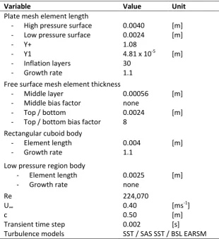
4.4 Numerical Simulation Set-up ... 45
4.4.1 CFD Uncertainty ... 48
4.5 Vortex Tracking ... 49
4.6 Results ... 50
4.7 Discussion ... 58
4.8 Conclusions ... 63
4.9 Recommendations ... 63
4.10 Future Work ... 64
4.11 Acknowledgements ... 64
4.12 Chapter Summary... 64
Chapter 5
The effect of submergence on the tip vortex of a t-foil hydrofoil ...67
5.1 Abstract ... 68
5.2 Introduction ... 69
5.3 Experimental methodology ... 73
5.3.1 PIV setup ... 74
5.3.2 Experimental uncertainty ... 76
5.3.3 Measurement of the velocity field ... 77
5.4 Results ... 79
5.5 Discussion ... 88
5.5.1 Hydrodynamic coefficients ... 88
5.5.2 Validation of PIV against the force measurements ... 90
5.5.3 Vortex smoothing correction due to aperiodicity ... 90
5.5.4 The effect of submergence on wing tip vortex circulation ... 91
5.5.5 Vortex diameter ... 92
5.5.6 Velocity profiles ... 92
5.5.7 Wing end cap geometries ... 93
5.5.8 Implications of the research ... 93
5.6 Conclusions ... 94
5.7 Future work ... 95
5.8 Acknowledgements ... 96
Chapter 6
Wing tip vortex ventilation of a T-foil hydrofoil at low submergence ...98
6.1 Abstract ... 99
6.2 Introduction ... 100
6.3 Methodology ... 102
6.4 Results ... 106
6.5 Discussion ... 131
6.5.6 Conclusions ... 140
6.5.7 Future work ... 140
6.5.8 Acknowledgements ... 141
6.6 Chapter summary ... 141
Chapter 7
Conclusions ... 143
7.1 Recommendations ... 145
7.1.1 Application –Avoiding and controlling tip vortex ventilation ... 145
7.1.2 The affect of surface waves on foil performance and tip vortex ventilation ... 146
7.2 Future work ... 147
Bibliography ... 149
Appendix A. Correction of PIV data for carriage vibration ... 156
Appendix B. Variables of the PIV uncertainty analysis using the ITTC guideline
7.5-01-03-03... 158
Appendix C. Image sequence and wake age ... 159
Appendix D. Image Plates ... 160
Appendix E. Multimedia file ... 205
Appendix F. Multimedia file ... 206
List of Figures
Figure 1-1. Hi-speed ferry hydrofoil vessels (A) Dihedral type - ‘Flying Dolphin Zeus’ ©Arno Winter (B) t-foil type – ‘Seven Islands Yume’ ©Tokai
Kaisen Ltd ... 3 Figure 1-2. Hydrofoil sailing craft (A) Emirates Team New Zealand ©Cameron
and (B) the ‘Blade Rider’, International Moth derivative ©Virginia
Veal ... 4 Figure 1-3. Mechanisms of hydrofoil ‘tip’ and ‘strut’ ventilation ... 6 Figure 2-1. Raw particle images from Chittiappa Muthanna, Di Felice, Verhulst,
Delfos, and Borleteau (2010).(A) Specula reflection resulting from saturation of the image sensor and (B) minor reflection within the
sensitivity of the image sensor ... 12 Figure 2-2. Time averaged PIV velocity fields obtained adjacent to a flat plate test
geometry with the flow direction normal to the image plane. The red dashed line marks the perimeter of the flat plate test geometry (A) Example of how a flow field may become corrupted by specula reflection. The affected part of the image is shown in white. (C Muthanna, Di Felice, Michiel, Delfos, & Borleteau, 2010) (B) Flow field obtained using fluorescent PIV showing no signs of specula
reflection. (Ashworth Briggs, Fleming, Ojeda, & Binns, 2014) ... 12 Figure 2-3. Nd:YAG emission (Ocean_Optics_Inc, 2014), Rhodamine 6G (R6G)
absorption and emission (Berngruber, 2015), and transmission
spectra for the 590 nm orange bandpass filter (MidOpt, 2017) ... 13 Figure 2-4. Dependence of amplitude ratio (η), on Stokes number (Ns),for
particles flowing in water and for several values of density ratios.
Reproduced from the results of Novotny and Manoch (2012) ... 17 Figure 2-5. Dependence of phase lag (β) on Stokes number (Ns),for particles
flowing in water and for several values of density ratios. Reproduced
from the results of Novotny and Manoch (2012) ... 17 Figure 2-6. Dependence of Stokes number (Ns), on frequency (f) for a range of
particle size in microns. Reproduced from the results of Novotny and
Manoch (2012) ... 18 Figure 2-7. RMS uncertainty in the PIV cross correlation with respect to particle
image diameter for a range of interrogation window sizes. Simulated data for single exposure/double frame data acquisition. Reproduced
Figure 3-1. Carriage mounted air filled periscope (A) 3D view (B) Section view ... 27 Figure 3-2. Experimental setup schematic for towing tank carriage mounted PIV. ... 27 Figure 3-3. Position of planes captured in relation the trailing edge datum using
2D PIV. ... 28 Figure 3-4. Double frame raw images from measurement plane 1 showing the
absence of reflection from the test geometry and dense high contrast
seeding (A) First pulse and (B) Second pulse ... 29 Figure 3-5. Raw images where the light sheet does not intersect the test
geometry from the HTA study (A) INSEAN (C Muthanna et al., 2010),
(B) MARIN (C Muthanna et al., 2010) and (C) AMC. ... 30 Figure 3-6. 2D velocity vectors plots averaged over 128 double frames on an 8 x
8 grid ... 31 Figure 3-7. Experimental results from the HTA and AMC showing the magnitude
of the (A) W and (B) V velocity with reference to the vortex centre. ... 31 Figure 4-1. Setup of the PIV physical experimental setup mounted on the towing
tank carriage (A) 3D view and (B) Plan view ... 41 Figure 4-2. Carriage mounted periscope (A) 3D view and (B) Section view ... 42 Figure 4-3. (A) Schematic representation of the multiphase fluid domain (B)
Mesh refinement schematic diagram ... 47 Figure 4-4. CFD and experimental vortex tracking methodology ... 50 Figure 4-5. Experimental planar velocity fields averaged over 128 double frames
for each of the measurement planes. High fidelity results are obtained up to the boundary of the test geometry using fluorescent
PIV. ... 52 Figure 4-6. Cross velocity fields displaying normalized vectors obtained at x/c
0.2 downstream from the trailing edge of the geometry for (A) BSL EARSM steady state result, fine grid and (B) PIV time average of 128
frames. ... 52 Figure 4-7. Experimental and numerical results for the (A)W and (B) V velocity
components measured from the centre of the vortex plotted against benchmark data (Bortleteau et al., 2009; Towers et al., 1999) on a plane at x/c 0.2 downstream from the trailing edge. The combined experimental and PIV uncertainties of and are shaded in grey, with the uncertainty in position for the SST result indicated with error bars. The BSL EARSM model results in the closest fit to the
Figure 4-8.W velocity fields for each measurement plane from the PIV results
(The white area is the masked test geometry) ... 53 Figure 4-9. Profiles of the velocity components with position normalised to the
vortex centre location at each measurement plane. (A)V and (B)W.
Error bars indicate the combined experimental and PIV uncertainties
of and . ... 54 Figure 4-10. Velocity fields with vortex structures displayed using the Lambda-2
criterion of -7.8 s-2. (A) SST, (B) SAS SST and (C) BSL EARSM. The SAS
SST model appears to enable a more complex flow topology with the persistence of eddies into the free stream, while the explicit solution
of the BSL EARSM model results in a simplified flow topology. ... 54 Figure 4-11. Movement of vortex structures and velocity field changes using the
Lambda-2 criterion of -7.8 s-2 for the SAS SST model. (A) t = 0 s, (B)
t+1/24 s, (C) t+1/12 s ... 55 Figure 4-12. Time histories measured at x/c 0.2 downstream from the trailing
edge showing.7 (A) Experimental variation of vortex Core
yz and(B)
CFD SST and SAS SST variation of Uyz, fine grid. The combined
uncertainty in position for the experiment is within the thickness of
the lines. ... 55 Figure 4-13. Samples from the time histories of the CFD SAS SST results
measured at x/c 0.2 downstream from the trailing edge showing the vortex centre Coreyz along the y and z axes.7Uyzremains within the
bounds indicated by the black dashed lines at 0.5 times the vortex
core diameter either side of the point Coreyz. (A) z axis and (B) y axis. ... 56
Figure 4-14. Vortex cross shift, cross velocity and cross acceleration. (A) Coreyz
PIV results, sample rate of 15 Hz (B) Uyz CFD SAS SST fine mesh,
sample rate of 500 Hz (C) Uyz CFD SAS SST fine mesh, resampled at 15
Hz. ... 56 Figure 4-15. Cross velocity and the acceleration of the stream-wise velocity
component of the vortex core. (SAS SST turbulence model, fine mesh,
Time step =0.002s, filter centered 400 time step moving average) ... 57 Figure 4-16. (A) The axial velocity calculated from the U and cross velocity
components and (B) Stream-wise and axial velocities within the vortex core. Addition of the cross velocity component shows the effect of vortex wander and kinks on the axial velocity of the core. Axial velocity peaks at 2.2 times the free-stream velocity (SAS SST turbulence model, fine mesh, Time step =0.002s, Filter centered 400
Figure 5-1. (A) The sections of the t-foil geometry are NACA 0012, the horizontal lifting surface has an AoA of 8o and (B) The 6 DOF force balance on
the towing tank carriage is translatable in the direction of the free stream, and the submergence of the t-foil can be varied while
maintaining a constant AoA. ... 74 Figure 5-2 (A) Light sheet intersecting the test geometry. Flow media is clearly
illuminated by the light sheet (B) The rounded and square wing cap geometries. The rounded cap is formed through a solid body of
revolution of the wing section. ... 74 Figure 5-3. Schematic diagram of the PIV experimental setup with the periscope
housing removed to clarify the location of the camera and mirror. The 6DOF force balance was located directly above the t-foil. Both the t-foil and periscope were mounted on linear rails to facilitate the
adjustment of immersion. ... 75 Figure 5-4. (A) The experimental setup on the towing tank carriage. Mid frame -
a black shroud covers the 6DOF balance and t-foil, bottom left - the periscope mounting, top right - the reservoir of seeding media and mid right - the laser head and (B) The periscope with fore and aft
fairings attached. ... 76 Figure 5-5. (A) Cross velocity uncertainty field with contours of cross velocity
magnitude, (B) 2D methods of identifying the vortex centre and (C)
Radial velocity with the vortex centre as the centre of rotation. ... 77 Figure 5-6. Hydrodynamic coefficients of the t-foil with square and round end
cap geometries including the vertical strut at an Rec 2.4x10⁵ or U∞ 2
ms-1 (A) The effect of change in submergence on CL and CD and (B)
Variation of L/D with change in submergence. At the deepest
submergence the L/D of the round end cap exceeds that of the square
end cap. ... 80 Figure 5-7. Vortex peak vorticity with respect to variation in CL, for the square
end caps. The change in vortex core vorticity is proportional to
variation in CLfor wake ages of between anx/c of 1 and 5. ... 81 Figure 5-8. Variation in vortex core vorticity with change in submergence for the
square end caps. Between an x/c of 0 and 1, the vorticity shed from the boundary layer of the wing into the trailing viscous wake sheet
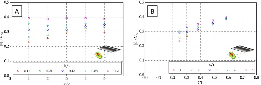
rolls up into the tip vortex. ... 81 Figure 5-9. Change in tip vortex maximum velocity magnitude (A) with
progression downstream from the t-foil and (B) with respect to CL. AoA 8o and U∞ 2ms-1. For wake ages of between 1 and 5 x/c the rate of
Figure 5-10. The effect of submergence and wake age on (A) and (B) at the radius of the core. With the exception of submergence h/c 1.7, decreases with wake age. The rate of change of increases with
reduction in submergence. ... 83 Figure 5-11. Radial profiles of for wake ages of between x/c of 1 and 5 and all
h/c. Red – round tips and black - square tip. ... 83
Figure 5-12. Variation in circulation within the vortex core expressed as / with change in submergence at the radius of the core. The dissipation of circulation with wake age reduces with submergence, and at low
submergence the vortex appears to roll up more rapidly. ... 84 Figure 5-13. Comparison of tip vortex maximum velocity magnitude for round
and square end cap geometries. The round end cap results in higher
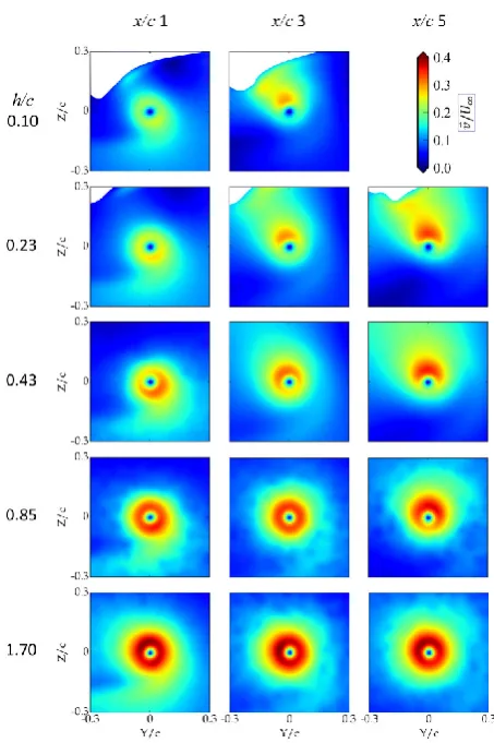
values of for all submersions ... 84 Figure 5-14. Images of velocity magnitude distribution for the square cap
geometry. From the PIV results, with reduction in submergence the velocity magnitude reduces and the distribution becomes
asymmetric. At the lower submergences the region of peak velocity magnitude located between the vortex and the free surface
strengthens with increase in wake age. Combined uncertainty of and f should be considered when viewing these results but has
been excluded to aid clarity of the presentation. ... 85 Figure 5-15. (A) V and (B) W velocity components obtained through slicing the
vortex vertically and horizontally respectively. Uncertainty is shown
by the shaded bands of ±2σ. ... 86 Figure 5-16. Extreme values of the velocity components obtained through slicing
the vortex vertically and horizontally respectively. (A) V component and (B) W component. With increase in wake age the V component for each submergence appear to converge in the region between the vortex and the free surface and to diverge below the vortex, whereas little variation in the W component is apparent on either side of the vortex with increase in wake age. With reduction in h/c the rate of
change of the V component increases. ... 87 Figure 5-17. (A) Vorticity, (B) Residual vorticity and (C) Strain rate tensor for
square and round wing end caps at an x/c of 0, for h/c 0.11, 0.43 and 0.85. The band of vorticity dominated by shear inboard of the vortex is both more contiguous and thicker for the round end cap. The tip vortex generated by the square end cap is larger and less intense than the round end cap. The strain rates of the two tip vortices are
Figure 6-1. Experimental setup (A) Force balance, submergence and interface plate (B) The Davidson Laboratory high speed towing tank showing the supports for the t-foil interface plate with AoA adjustment in the
foreground... 103 Figure 6-2. Measurement of image scales showing the submergence and wake
age datums used in this study ... 104 Figure 6-3. Viewed obliquely from below the typical surface wake of a t-foil at
AoA 8, h/c 0.22, and U∞ 4 ms-1 ... 105
Figure 6-4. Traces of vortex paths at AoA 8, h/c 0.43, and U∞ 10 ms-1 ... 106
Figure 6-5. Variation of hydrodynamic coefficients with respect to change in AoA
at ... 107 Figure 6-6. Lift polar for the t-foil with square wing end caps at h/c 3.4 ... 107 Figure 6-7. Viewed from above, the surface wake behind a t-foil at low
submergence is complex, with interacting wake systems from the strut and wing tips combined with surface perturbation caused by
the strut spray... 109 Figure 6-8. Viewed obliquely from below, increase in velocity results in the
donstream extension of straight section of strut wake AoA 8, h/c 0.43,
U∞ 2, 4 & 6 ms-1. ... 110
Figure 6-9. Descending entrained bubbles highlight the strut interface vortices. AoA 8°, h/c 0.43, and U∞ 4 ms-1. Filament cavities are visible at 0.9 and
1.2 s ... 113 Figure 6-10. Ventilated strut vortex cavities. AoA 8, h/c 0.43, and U∞ 6 ms-1.
Initially the strut vortices appear as coherent structures with a highly non-uniform fluid interface that descend from the surface wake. With increase in wake age, the cavities briefly stabilise before expanding and separating into discontinuous cavities. At 0.9s straight sections
of tip vortex cavity become visible above the strut vortices. ... 115 Figure 6-11. Tip vortex filament cavitation or incompletely ventilated cavities
with ventilated strut cavities. AoA 8, h/c 0.43, and U∞ 10 ms-1 . The tip
vortices are elucidated by a descending pair of coherent structures with small diameter, that originate from further forward on the tip wave wake than is visible at 6 ms-1. To the rear of this a second pair
of irregular structures of larger diameter than the previous appear
close to the free surface. ... 117 Figure 6-12. Ventilated tip and strut vortex cavities. AoA 8, h/c 0.43, and U∞ 12
ms-1. The tip vortices appear as coherent structures with a highly
vortices are visible as a rope of coalesced bubbles between the tip
vortices and the free surface... 119 Figure 6-13. Cavitation bubbles in the low pressure region of the horizontal foil
at submergence h/c 0.22, AoA 8°. (A) U∞ 8 ms-1 (B) U∞ 10 ms-1 (C) U∞
12 ms-1 ... 119
Figure 6-14. Cavity development with change of submergence at AoA° 8 and U∞
8ms-1. (A) h/c 0.22 both thick filament and rope-like cavities, (B) h/c
0.43 short sections of filament cavities, (C) h/c 0.85 very short
filament cavities. ... 121 Figure 6-15. Viewed from above, the development of cloud cavitation with
change in free stream velocity and submergence AoA 8° (A) h/c 0.22, U∞ 10 ms-1 (B) h/c 0.22, U∞ 12 ms-1 (C) h/c 0.43, U∞ 10 ms-1 (D) h/c
0.43, U∞ 12 ms-1 ... 122
Figure 6-16. Vertical displacements of the vortex wakes for foil submergence (A) h/c 0.22 (B) h/c 0.43. Greater submergence results in the increased
persistence of cavities downstream. ... 124 Figure 6-17. Depth of vortex wake paths for foil submergence (A) h/c 0.85 (B) h/c
1.70. At h/c 1.70 minimal trajectories are reported due to the absence of cavity formation. Test scenario h/c 1.70 at U∞ 12 ms-1 exceeded the
capacity of the load support. ... 125 Figure 6-18. Formation of cloud cavitation with change in velocity at AoA 8°, h/c
0.22, x/c 4. ... 127 Figure 6-19. Formation of cloud cavitation with change in velocity at AoA 8°, h/c
0.22, x/c 11.14 ... 128
Figure 6-20 AoA 8°, h/c 0.22, U∞ 2.0 ms-1, x/c 4 (A) cross velocity contours and
uncertainty field (B) particle image with countours of uncertainty in
cross velocity magnitude ... 129 Figure 6-21. AoA 8°, h/c 0.22, U∞ 4.5 ms-1, x/c 11 (A) cross velocity contours and
uncertainty field (B) particle image with countours of uncertainty in
cross velocity magnitude ... 129 Figure 6-22. View looking upstream toward the t-foil, cloud cavitation in the
hydrofoil tip wave wake is visible AoA 8, h/c 0.22, and U∞ 4.5 ms-1 ... 130
Figure 6-23. View looking through the side inspection window of the towing tank. Cavity formation within the tip vortex wave wake AoA 8, h/c
0.43, and U∞ 10ms-1 ... 130
Figure 6-24 Enlarged views of Figure 6-23. A vortex ring forms as a jet connects
Figure 6-25 Radial distribution of vortex circulation averaged accross x/c 1 to 5 at AoA 8° and U∞ 2 ms-1 (A) normalised by the bound circulation at
each depth of submersion (B) normalised by the circulation of a
deeply submerged case. ... 136 Figure 6-26. Radial variation in circulation averaged accross x/c 1 to 5 at an AoA
8° and U∞ 2 ms-1(A) with respect to hydrofoil submergence (B) with
respect to the baseline vortex circulation at an h/c of 1.70. ... 136 Figure 6-27. Vortex filament cavites of varying sizes wrapping the free surface of
a breaking wave. Reproduced with the kind permission of (A) Kenji
Croman ©Kenji Croman ... 139 Figure 6-28. Schematic diagram of hypothesised interaction between wave wake
vortices and the trailing tip vortex for a t-foil at low depth of
submersion ... 140 Figure B-7-1. Corrected instantaneous velocity field, normalised to the mean
List of Tables
Table 3-1. Location of vortex centre, calculated from U, Vand W velocities ... 31 Table 4-1 Propagation of uncertainties relevant to PIV ... 43 Table 4-2. Values of the variables applied for this PIV uncertainty analysis ... 44 Table 4-3. Sources of experimental uncertainty ... 45 Table 4-4. Variables used in the simulation setup for the fine grid ... 46 Table 4-5. Grid convergence metrics ... 49 Table 4-6. Vortex location wandering statistics for the experimental study and
CFD results for the fine grid ... 55 Table 4-7. Correlations between the changes in the location of Uyz and Coreyz, and
the axes of motion of Uyz and the axes of motion vortex centre (Fine
Nomenclature
Greek and Roman symbols
AoA Angle of incidence
c Chord length
Coreyz Vortex centre CL 3D Coefficient of lift CD 3D Coefficient of drag
D Drag force
dp Particle diameter
⃑ Curl of the velocity field
h Depth of submersion
h/c Depth of submersion in chord lengths
L Lift force
lr Physical distance of the reference point in mm Lr Image distance of the reference point in pixels lt Distance from camera to the image plane
p Local pressure
p∞ Ambient pressure
R Vortex core radius
Re Reynolds number
s Span
S Strain rate tensor
sp Standard deviation of the particle diameter
U Velocity component in the x or free stream direction
Ur Radial velocity
U∞ Free stream velocity
Uaxial Vortex core velocity aligned with the local vortex axis Ucore U component of the vortex core axial velocity
Uyz Point of extreme vortex core axial velocity local tangential velocity along the closed path Mean tangential velocity
V Velocity component in y W Velocity component in z
x Streamwise distance
x/c Wake age or streamwise distance in chord lengths y Horizontal distance normal to the freestream Y1 First layer height
Y+ Non-dimensional measure of the first layer thickness
z Vertical distance
Circulation
Circulation of the vortex at R Bound circulation of the hydrofoil Δt Time interval between frames
⃑ Relative error on Richardson extrapolated velocity curl
ρ Density
σ Standard Deviation
σ CD Uncertainty in CD
σ CL Uncertainty in CL
Uncertainty in cavity radius Uncertainty in carriage velocity
⃗ Uncertainty in cross velocity magnitude Combined uncertainty in position Uncertainty in x position
Uncertainty in y position Uncertainty in z position Streamwise vorticity tensor
⃑ Peak streamwise vorticity
Abbreviations
AMC Australian Maritime College
BSL EARSM Baseline Explicit Algebraic Reynolds Stress Model
CFD Computational Fluid Dynamics
EVM Eddy Viscosity Model
HTA Hydro Testing Alliance
INSEAN The Italian Ship Model Basin
ITTC International Towing Tank Conference
LES Large Eddy Simulation
LOA Length Overall
MARIN Maritime Research Institute Netherlands
PIV Particle Image Velocimetry
RANS Reynolds Averaged Navier Stokes
SAS SST Scale Adaptive Simulation Shear Stress Transport
SST Shear Stress Transport
URANS Unsteady RANS
Chapter 1
Introduction
1.1
Development of hydrofoils on monohulls in the 21
stcentury
Despite developments in the 21st century in hydrofoil systems on monohull yachts ranging in
that might be expected from a large monohull remains to be seen. With the quest for reduction in course times as a sole driver rather than specific point of sail performance gains, both ‘T’ and ‘L’ foil configurations have proved their superiority with alternative configurations left by the wayside as if by the process of Darwinism.
1.2
High performance hydrofoils
Historically, a large number of hydrofoil craft have been designed with surface piercing dihedral foils, which accommodate change in velocity, load and sea state through passive variation of the submerged foil area as the free surface intersection point varies in height. By the latter part of the 20th century, dihedral foils dominated early development of hydrofoil
craft (Figure 1-1), due to their simplicity of construction, lack of requirement for a control system and superior sea keeping characteristics. When compared with traditional high speed surface craft, vertical accelerations are reduced by nearly an order of magnitude in most sea states (Bhattacharyya, 1978).
Figure 1-1. Hi-speed ferry hydrofoil vessels (A) Dihedral type - ‘Flying Dolphin Zeus’ ©Arno Winter (B) t-foil type – ‘Seven Islands Yume’ ©Tokai Kaisen Ltd
The transition from dihedral, to vertical strut based foil systems, has been driven primarily by the obtainable performance gains. The use of ‘T’ and ‘L’ foils results in a further reduction in vertical accelerations (Bhattacharyya, 1978), and decrement in drag due to the simplified foil support structure (Figure 1-2). Wadlin, Ramsen, and McGehee (1950) and more recently Binns, Brandner, and Plouhinec (2008) demonstrated that minimisation of drag requires the hydrofoils to be at low submergence. T-foils in particular can suffer from sudden reduction in lift when operated close to the free surface, due to a phenomena known as ‘tip ventilation’ (Figure 1-3). Field test reports on the mechanisms involved in tip ventilation - where a ventilation pathway is believed to form between the free surface and hydrofoil through the core of the hydrofoil trailing tip vortex - are largely anecdotal – being based upon the personal accounts of sailors. The proprietary knowledge gained by Americas Cup design teams rarely makes it into the public forum leading to an absence of published research. Recently, interest to understand tip ventilation in order to remove the manifestation of control issues has rekindled, with the main forum at present being the America’s Cup and International Moth sailing craft shown in Figure 1-2.
Figure 1-2. Hydrofoil sailing craft (A) Emirates Team New Zealand ©Cameron and (B) the ‘Blade Rider’, International Moth derivative ©Virginia Veal
1.3
Problem definition
Tip ventilation via the wing tip vortex has been reported in both open water and laboratory experiments (TA Barden & Binns, 2012; Emonson, 2009; Ramsen, 1957). Ventilated cores have been observed to appear downstream of the wing tip, extending upstream toward the foil with time until a pathway is created to the hydrofoil tip. A brief ventilation event may result in a cavity trailing from the tip or control flap termination (Gulari, 2009), whereas in events of longer duration, ventilation may spread across the low pressure side of the hydrofoil causing a significant loss of lift which can cause control issues (Claughton, 2015) further leading to elevated structural loadings should a catastrophic loss of lift occur (Ashworth Briggs, Fleming, Ojeda, & Binns, 2014).
Wadlin et al. (1950) presented a study of the effect of submergence ratio and velocity on lift, followed shortly after with a parametric study by Ramsen (1957) on the appearance of fully ventilated flow (described as full bubble) using submergence ratio vs. Froude number for 3 models with all data collapsing to a single line. Ramsen (1957) described the forward progression of a trailing ventilated cavity until the occurrence of foil ventilation; however the depths of submergence, angles of attack and aspect ratio of the test geometry used in the study are largely incomparable with scenarios where tip ventilation has been observed to occur in modern day field tests.
A prerequisite for the ventilation of a hydrofoil is the existence of a region of low pressure. Such regions exist on the low pressure side of the hydrofoil and within the core of the wing tip trailing vortex. With sufficient pressure deficit the conditions for the existence of cavities, ventilated cavities - air-filled spaces - around the hydrofoil or in vortex filaments have been shown to occur. The occurrence of hydrofoil cavitation can be predicted with a priori knowledge of variables such as velocity, loading, ambient pressure, nuclei and gas content (Franc & Michel, 2004). Hoerner (1985) argued that scale is critical; at full scale, cavitation will occur earlier than for a model scale test hydrofoil, arguing that the onset of cavitation requires time for bubbles to grow around microscopic nuclei and that the relatively brief exposure of the fluid to a low pressure peak is proportional to x/U∞ where x is only a small fraction of the chord length.
The causes and mechanisms of tip ventilation inception are complex and not fully understood at present. Controlled experimental investigations of the inception of tip vortex ventilation have been largely restricted to depths of submergence of less than the ratio of depth/chord length (h/c) of 0.35, which are unrealistic for hydr
of foil egress from the water. mechanisms and sources of
ventilation remains a challenge for unpredictable nature of the phenomen
Figure 1-3. Mechanisms
1.4
Research question
o Does free surface proximity affect the o How and where does the inception of a o What topological changes
tip vortex?
1.5
Methodology
A qualitative investigation was undertaken NACA 0012 t-foil at a range
The causes and mechanisms of tip ventilation inception are complex and not fully at present. Controlled experimental investigations of the inception of tip vortex ventilation have been largely restricted to depths of submergence of less than the ratio of
) of 0.35, which are unrealistic for hydrofoil operation d
foil egress from the water. While it is clear why a cavity forms within the tip vortex, the ventilation inception at operational submergence are not ventilation remains a challenge for high speed foil borne craft due to the apparently
the phenomenon.
Mechanisms of hydrofoil ‘tip’ and ‘strut’ ventilation
Research questions
oes free surface proximity affect the flow topology of the tip vortex? How and where does the inception of a tip vortex ventilation event initiate?
topological changes occur during interaction between the free surface and the
investigation was undertaken through observation of trailing cavities using a foil at a range of velocities between 2 and 12 ms-1 and
The causes and mechanisms of tip ventilation inception are complex and not fully at present. Controlled experimental investigations of the inception of tip vortex ventilation have been largely restricted to depths of submergence of less than the ratio of oil operation due to the risk While it is clear why a cavity forms within the tip vortex, the at operational submergence are not. Tip due to the apparently
ventilation
of the tip vortex? ventilation event initiate?
occur during interaction between the free surface and the
submergence h/c of between 0.22 and 1.70. Furthermore, the trajectories, formation and break-up of the trailing tip vortices were evaluated quantitatively.
Using a carriage mounted Particle Image Velocimetry (PIV) system, the two dimensional flow field normal to the free stream was quantified at a velocity of 2 ms-1. Metrics of
circulation, tangential velocity and peak cross-velocity magnitude were compared for a range of submergence h/c of between 0.11 and 1.70.
1.6
Novel Aspects
o This investigation provides a contribution to the understanding of tip vortex ventilation inception through:
o Investigation of the tip vortex wake generated by a t-foil in close proximity to the free surface. Carroll (1993) investigated the trailing tip vortex from a vertical foil with the tip proximate and normal to the free surface at a single depth of submersion.
o Near, mid and far field quantitative results for vertical wake location and cavity formation for a t-foil in close proximity to the free surface. Published work (Devenport, Rife, Liapis, & Follin, 1996; McAlister & Takahashi, 1991; Oh & Suh, 2009) has been focused on deeply submerged cases, either in the near field or the extreme far field .
o Characterisation of the tip vortex generated by a t-foil in close proximity to the free surface through velocity fields obtained using fluorescent PIV.
o Highlighting the presence of strut intersection vortices and their interaction with the trailing tip vortices.
o Highlighting a relationship between vortex aperiodicity and fluctuation in vortex axial velocity.
1.7
Significance of the research
knowledge may lead to downstream reduction in peak loads for fluid-structure interactions involving foil devices for energy capture, flight and propulsion, leading to extended fatigue life, weight saving, energy efficiency, reduction in acoustic signature and reduction in energy costs. With respect to foil borne craft, an increased level of passenger comfort and security can be anticipated with additional benefits of improved fuel efficiency and reduction in transport times.
1.8
Thesis outline
This thesis has been divided into chapters. Where a chapter has been submitted for publication, the journal has been clearly stated and the status of the submission indicated. The general structure of this thesis is as follows:
Chapter 1 Presents the gap in knowledge and outlines how the investigation has been undertaken. Literature reviews on the specific elements of the study can be found within the introduction of each chapter.
Chapter 2 Discusses the use of fluorescent seeding particles for PIV and how this may affect the fidelity of the data acquired. A methodology for the appropriate selection of particle size and density is presented.
Chapter 3 Describes the benchmarking of fluorescent PIV against experimental studies
in similar test facilities, using a surface piercing flat plate at incidence on the moving carriage of the Australian Maritime College towing tank. High fidelity velocity fields were obtained using fluorescent seeding media.
Chapter 4 Compares values of vortex aperiodicity obtained from numerical studies with
Chapter 5 Investigates the effect of t-foil submergence on the flow field of the trailing tip vortex for two wing tip geometries. The tangential velocities, peak cross-velocity magnitudes and circulations are compared.
Chapter 6 Presents new observations of a t-foil hydrofoil in close proximity to the free
surface, including tip mechanisms of vortex ventilation at low submergence.
Chapter 7 Summarises the knowledge gained in each work package and presents
conclusions and recommendations for future work.
Appendix A Correction for velocity field artefacts due to carriage vibration
Appendix B Variables for PIV uncertainty analysis using the ITTC guideline 7.5-01-03-03
Appendix C Image sequence and wake age
Appendix D Image plates at AoA 8°
Appendix E Multimedia file showing a tip vortex cavity intermittently advancing
Appendix F Multimedia file showing cloud cavitation through a particle image
Chapter 2
Fluorescent Particle Image
Velocimetry
Theunissen (2012) emphasised the challenge of obtaining flow field measurements adjacent to fluid structure interfaces with an editorial in the Journal of Aeronautics and Aerospace Engineering. This obstacle, fundamentally limits the ability to characterise the coupling, and obtain an understanding of the underlying physics. In test cases with dynamic boundaries, the use of fluorescent seeding is a particular advantage, due to the difficulties in optimising the camera viewing angle to reduce reflection.
2.1
PIV
PIV may be used to non-intrusively obtain instantaneous two and three dimensional measurements of a flow field. In its simplest form, the process of PIV involves the acquisition of raw particle images, where the tracer particles have been selected to closely follow the flow under investigation. The raw images are subdivided into multiple interrogation regions and the displacements of particles within these regions measured between two consecutive frames of known inter-frame interval. The resulting output is a displacement vector within each interrogation window, which when combined form a velocity field. For further information on the PIV technique the reader is referred to Raffel, Willert, Werely, and Kompenhans (2007).
In the typical operating conditions of a foil near a free surface, bubbles due to vortex filament cavitation, tip ventilation, strut ventilation or entrainment through wave action may be present. Acquisition of a flow field data adjacent to such bodies using PIV is often restricted due to specula reflection from the laser light sheet as shown in Figure 2-1A from polished surfaces, curved surfaces, air/water interfaces such as bubbles or the free surface leading to over exposure and possible damage to the image sensor (Schröder, 2008). In Figure 2-2A specula reflection is indicated by the white region, whereas in Figure 2-2A only the test geometry obscures the velocity field.
2.1.1
Fluorescent PIV
Figure 2-1. Raw particle images from Chittiappa Muthanna, Di Felice, Verhulst, Delfos, and Borleteau (2010).(A) Specula reflection resulting from saturation of the image sensor and (B)
minor reflection within the sensitivity of the image sensor
Figure 2-2. Time averaged PIV velocity fields obtained adjacent to a flat plate test geometry with the flow direction normal to the image plane. The red dashed line marks the perimeter of the flat plate test geometry (A) Example of how a flow field may become corrupted by specula reflection. The affected part of the image is shown in white. (C Muthanna, Di Felice, Michiel, Delfos, & Borleteau, 2010) (B) Flow field obtained using fluorescent PIV showing no
signs of specula reflection. (Ashworth Briggs, Fleming, Ojeda, & Binns, 2014)
A
B
Figure 2-3. Nd:YAG emission emission (Berngruber, 2015)
2.1.2
Particle size
Tracer particles used in PIV experiments vary widely millimetres in diameter, the latter used in large scale expe
where achieving an adequate signal to noise ratio may have been challenging. The density the tracer particles varies greatly and in many cases selection may
availability and cost of materials.
reader in determining the tracking accuracy this study have a mean diameter
of flow media used in many PIV studies.
2.1.3
Stokes number
So as to accurately capture the flow field
path line as closely as possible. Stokes law characterises the behaviour suspended in a fluid and is
equation 2-6, using the difference between the fluid and particle velocities (Melling, 1997).
. Nd:YAG emission (Ocean_Optics_Inc, 2014), Rhodamine 6G (R6G)
(Berngruber, 2015), and transmission spectra for the 590 nm orange bandpass filter (MidOpt, 2017)
Tracer particles used in PIV experiments vary widely, from less than a micron to several millimetres in diameter, the latter used in large scale experiments involving
where achieving an adequate signal to noise ratio may have been challenging. The density the tracer particles varies greatly and in many cases selection may be
materials. Often, little or no information is provided to assist the reader in determining the tracking accuracy of the experiments. The tracer particles used in this study have a mean diameter of 57 microns, falling toward the lower bounds
n many PIV studies.
So as to accurately capture the flow field, the particle path line should be matched to the fluid path line as closely as possible. Stokes law characterises the behaviour
suspended in a fluid and is applicable when the Reynolds number (Re) using the difference between the fluid and particle velocities
, Rhodamine 6G (R6G) absorption and , and transmission spectra for the 590 nm orange bandpass
from less than a micron to several involving wind turbines where achieving an adequate signal to noise ratio may have been challenging. The density of be influenced by the little or no information is provided to assist the the experiments. The tracer particles used in 57 microns, falling toward the lower bounds of the range
where ν is kinematic viscosity of the fluid, which is used when the density of the fluid f is
equal to the density of the particle p , and is the characteristic length and diameter of the
seeding particle.
Stokes number (Ns) calculated from equation 2-6 characterises the behaviour of particles suspended in a fluid. For a high degree of coupling or ability to match the fluid flow with an error of less than 1%, a Stokes number of <<0.1 is recommended (Tropea, Yarin, & Foss, 2007).
=
(2-2)where is the particle relaxation time.
Stokes number may also be defined as in equation 2-6,
=
w
n
(2-3)
where ω is angular velocity corresponding to the maximum frequency of disturbances in the flow.
Assuming a drag profile for a spherical particle, the relaxation or response time of the particle describes the time taken for a particle to reach 63.2% of the fluid velocity , while 99% of is achieved in 4.5 (Novotny & Manoch, 2012).
=
where is the particle density, the particle diameter and the fluid dynamic viscosity.
The frequency response of high density particles is poor, whereas low density particles will over respond. Should particle density equal the fluid density then equation 2-6 simplifies to equation 2-5 and the difference in phase lag and amplitude between the particles and the fluid will be zero.
=
18
(2-5)
2.1.4
Non spherical particles
Irregularly shaped small particles are commonly treated as spheres with a fluid-dynamically equivalent diameter (Melling, 1997). To obtain the aerodynamic diameter ( ), a dynamic shape factor (χ) calculated from equation 2-6, is applied to Stokes law which accounts for the effect of irregularity in shape and is defined as the ratio of the resistance force of the irregularly shaped particle to that of a sphere with the same volume and velocity (Hinds, 2012). The of an irregularly shaped particle is defined as the diameter of a sphere with a density of 1000 kg/m3 and the same settling velocity as the irregular particle and is calculated from equation 2-6.
χ =
3 (2-6)
where is the drag force, and is the diameter of a sphere with an equal volume to that of the irregular particle.
=
=
χ (2-7)
where is the standard particle density of 1000 kg/m3.
2.1.5
Particle density
Applying the concept of the energy transfer function to instantaneous particle and fluid motion, Melling (1997) references Chao (1964), demonstrating that for neutrally buoyant particles the energy transfer functions of the particles and fluid are equal and the particles will exactly trace the fluid motion.
Novotny and Manoch (2012) presented a methodology for determining the tracking accuracy for a given flow regime to aid tracer particle selection in PIV experiments. This methodology has been applied in this study due to the simplicity and the limitation it places with respect to the maximum frequency of the disturbances in the fluid that can be measured. The process is outlined in the following section.
2.1.6
The Novotny methodology for particle selection
Figure 2-4. Dependence
(Ns),for particles flowing in water and for several values density ratios. Reproduced from the results
Figure 2-5. Dependence
particles flowing in water and for several values ratios. Reproduced from the results
Dependence of amplitude ratio (η), on Stokes number for particles flowing in water and for several values of
density ratios. Reproduced from the results of Novotny and Manoch (2012)
Dependence of phase lag (β) on Stokes number (Ns
particles flowing in water and for several values of density ratios. Reproduced from the results of Novotny and Manoch (2012)
Stokes number of
Novotny and Manoch (2012)
Figure 2-6. Dependence of Stokes number
microns. Reproduced from the results
Using the method presented
mean diameter and a required accuracy a Stokes number of 0.15. Based on approximately 0.3, and from approximately 1 kHz.
2.1.7
Particle image size
Particle image size – the size important from the perspective image size is smaller than the size toward integer values of pixel Probability Density Function (PDF) (LaVision, 2012). The case of
0 and 1 px displacement on the histogram, whereas peak locking distribution between these values.
When the particle image size is greater than the image pixel obtained. Raffel et al. (2007)
to a reduction in the RMS uncertainty in the cross correlation.
Stokes number (Ns), on frequency (f) for a range microns. Reproduced from the results of Novotny and Manoch (2012)
Using the method presented above, in the case of neutrally buoyant particles mean diameter and a required accuracy for the amplitude ratio of 99%, Figure Based on Figure 2-5, a Stokes number of 0.15 returns
approximately 0.3, and from Figure 2-6 we find a maximum frequency response
the size of the particle image in pixels (px) on the imaging sensor important from the perspective of the uncertainty of the velocity field. When the par
the size of the sensor pixel, peak locking occurs,
pixel displacement. Peak locking can be monitored from the Probability Density Function (PDF) of the pixel displacements of the velocity components
of no peak locking will appear as a uniform distribution between displacement on the histogram, whereas peak locking results in
these values.
When the particle image size is greater than the image pixel size sub pixel resolution can be demonstrated that optimisation of the particle image size leads to a reduction in the RMS uncertainty in the cross correlation.
for a range of particle size in Novotny and Manoch (2012)
neutrally buoyant particles of 57 micron Figure 2-4 indicates returns a phase lag of frequency response of
on the imaging sensor – is the velocity field. When the particle resulting in a bias displacement. Peak locking can be monitored from the the velocity components no peak locking will appear as a uniform distribution between results in a bias in the
Figure 2-7 shows that for single exposure/double frame PIV a decrease in the size correlation window results in a reduction in the optimal particle image diameter at the minimum value of the RMS uncertainty.
Figure 2-7. RMS uncertainty in the PIV cross correlation with respect to particle image diameter for a range
exposure/double frame data acquisition.
In this study, the mean particle pixel size was calculated as 1.5 px, which using the data presented by Raffel et al. (2007)
correlation window of 16 x 16 px for single exposure
Neutrally buoyant materials provide a limited opportunity to tailor the optical setup through variation of the particle size,
view, other than by aperture
2.1.8
Particle Image Density
The volumetric density and homogeneity
velocity components through the measurement volume combine to affect the particle image density of the captured images and
Adrian (1991) determined that the probability
shows that for single exposure/double frame PIV a decrease in the size correlation window results in a reduction in the optimal particle image diameter at the
uncertainty.
RMS uncertainty in the PIV cross correlation with respect to particle image diameter for a range of interrogation window sizes. Simulated data for single
a acquisition. Reproduced from the results of Raffel
the mean particle pixel size was calculated as 1.5 px, which using the data Raffel et al. (2007) results in an RMS uncertainty of approximately 0.05 px for a 16 x 16 px for single exposure/double frame data acquisition. Neutrally buoyant materials provide a limited opportunity to tailor the optical setup through
in order to vary the particle image size for the required field control as described by Adrian (1997).
Particle Image Density
The volumetric density and homogeneity of the tracer particle dispersion, particle shift velocity components through the measurement volume combine to affect the particle image
the captured images and thus affect the probability of valid detection.
ermined that the probability of valid detection deteriorates as particle shows that for single exposure/double frame PIV a decrease in the size of the correlation window results in a reduction in the optimal particle image diameter at the
RMS uncertainty in the PIV cross correlation with respect to particle image interrogation window sizes. Simulated data for single
Raffel et al. (2007)
the mean particle pixel size was calculated as 1.5 px, which using the data approximately 0.05 px for a double frame data acquisition. Neutrally buoyant materials provide a limited opportunity to tailor the optical setup through in order to vary the particle image size for the required field of
image density reduces or an increased proportion of seeding media moves out of the measurement volume, due to either in plane or through plane motion.
2.1.9
In plane loss
In plane loss of particle image density is due to the planar particle image shift of particle pairs out of the interrogation window between frames. The magnitude of the particle image shift affects the minimum size of the interrogation window that can be used, with the probability of valid detection falling due to the reduction in particle pairs. For a given flow, reduction of the interframe interval will reduce the particle image shift and hence enable the use of a smaller interrogation window. In general in plane particle displacement should be limited to <25% of the interrogation window size. For this study, a 25% particle shift and interrogation window size of 16 x 16 px, with between 6 and 7 particle pairs achieving a 95% probability of valid detection was determined based on the simulations by Raffel et al. (2007).
2.1.10
Out of plane loss
When considering 2D PIV, out of plane loss of correlation is due to the effect of flow perpendicular to the light sheet and is linearly related to the reduction in particles recorded in both images. To obtain a valid detection probability of > 95%, 75% of the original particle pairs must remain within the thickness of measurement volume illuminated by the light sheet, resulting in > 5 particle pairs per interrogation window for single exposure/double frame PIV (Raffel et al., 2007). Control of this fraction is achieved through variation of the interframe interval, such that the through plane particle displacement is < 25% of the light sheet thickness. Discussion of methods used to account for highly three dimensional flows in the PIV setup and post processing can be found in Raffel et al. (2007), p.176.
2.1.11
Interframe interval
light sheet thickness. Δt may then be reduced to control the size of the interrogation window, providing due consideration to the signal to noise ratio is made.
2.2
Particle Image Velocimetry Limitations
The limitations of PIV with respect to this study are outlined in the following sections.
2.2.1
Swirling and shear flows
In certain cases, such as in swirling or high shear flows, additional body forces act upon the tracer particles. In the case of swirling flows, if particle density is incorrect the tracers will slip through the fluid as the drag provides inadequate centripetal force to maintain the location of the tracer particles within the fluid (Melling, 1997). In Chapters 5 of this thesis, radial slip has been evaluated by quantification of the radial velocity component in the flow field of the wing tip vortex core.
2.2.2
Seeding and management of tracer particle dispersion
2.2.3
PIV system installation on a moving carriage
The PIV equipment was rigidly mounted and braced to the towing tank carriage to minimise local inertial effects on the test equipment caused by random carriage motions. Minor effects on the velocity fields, due to rigid body motion of the carriage were then post processed from the results as described in Appendix A. The camera and light sheet were adjustable on linear rails aligned with the z-axis, with the relative separation between the camera and light sheet on the x and y axes fixed throughout each study, in order to maintain a constant measurement volume and minimise the number of image calibrations required. The position of the test geometries along the X axis was adjustable so as to enable acquisition of multiple streamwise measurement planes. Upstream effect of the periscope on the flow field might be ascertained using a non intrusive measurement of the flow field in the future using the technique of Laser Doppler Velocimetry to measure the flow field both with and in the absence of the periscope.
Chapter Summary
In this chapter the methodology of particle selection and the setup parameters for 2D PIV have been described. Fluorescent PIV has been discussed, and shown to result in high fidelity velocity fields in challenging conditions. Neutrally buoyant particles have been shown to provide an opportunity to optimise the PIV setup parameters, permitting greater freedom in the selection of particle size.
Chapter 3
Benchmarking Particle Image
Velocimetry on the Moving Carriage of the
Towing Tank
This chapter presents the study used to benchmark PIV on the moving carriage of the Australian Maritime College. The citation for the research article is:
Ashworth Briggs, A., Fleming, A., Ojeda, R., & Binns, J. (2014). Tracking the vortex core from a
surface-piercing foil by Particle Image Velocimetry (PIV) Using Fluorescing Particles Paper pre-sented at the 19th Australasian Fluid Mechanics Conference Melbourne, Australia
The following conference paper was presented at the 19th Australasian Fluid Mechanics Conference, in Melbourne, Australia, 8-11th December 2014. The manuscript has been
reformatted otherwise it has been included without alteration.
3.7
Chapter Summary
In this chapter the methodology for using PIV on the moving towing tank carriage at the AMC has been described and benchmarked against previous experimental studies by INSEAN and MARIN in similar test facilities. The capability of capturing high fidelity velocity fields in a challenging environment using in-house manufactured fluorescent seeding media adjacent was demonstrated.
Chapter 4
Tracking the vortex core from
a surface-piercing flat plate by Particle
Image Velocimetry for numerical
valida-tion.
This chapter was accepted in March 2018 and the unedited manuscript included in this thesis incorporates the reviewer’s comments. The citation for the research article is:
Ashworth Briggs, A., Fleming, A., Duffy, J. & Binns, J.R. (2018). Tracking the vortex core from a
surface-piercing flat plate by particle image velocimetry and numerical simulation. Proceedings of
the Institution of Mechanical Engineers, Part M: Journal of Engineering for the Maritime
Envi-ronment.
In the previous chapter, PIV on the moving towing tank carriage at the AMC was benchmarked against published experimental results, and in-house manufactured fluorescent seeding medium was demonstrated to be capable of achieving the acquisition of high fidelity velocity fields.
In this chapter the validity of two numerical turbulence models – the Menter Shear Stress Transport model (SST) and the recent Scale Adaptive Simulation Shear Stress Transport model (SAS SST), using the volume fraction method and CFX solver – are evaluated with attention to the persistence and behaviour of swirling flows as they move down stream, away from the test geometry. The feasibility of addressing the research topic solely through numerical simulation is also considered.
4.1
Abstract
The wake flow around the tip of a surface piercing flat plate at an angle of incidence was studied using 2D Particle Image Velocimetry (PIV) as part of benchmarking the PIV technique on the moving carriage in the Australian Maritime College (AMC) towing tank. PIV results were found to be in close agreement with those of the benchmarking work presented by the Hydro Testing Alliance (HTA), and a method of tracking the tip vortex core near a free surface throughout numerical simulation has been demonstrated. Issues affecting signal to noise ratio, such as specula reflections from the free surface and model geometry were overcome through the use of fluorescing particles and a high pass optical filter.
Numerical simulations using the ANSYS CFX Solver with the volume of fluid (VOF) method were validated against the experimental results, and a methodology developed for tracking the location of the wandering vortex core experimentally and through simulation. The ability of the Scale Adaptive Simulation Shear Stress Transport (SAS SST) turbulence model and the Shear Stress Transport (SST) model to simulate three dimensional flow with high streamline curvature was compared. The SAS SST turbulence model was found to provide a computationally less resource intensive method of simulating a complex flow topology with large eddies, providing an insight into a possible cause of tip vortex aperiodic wandering motion. At high angles of attack vortex shedding from the leading edge separation of the test geometry is identified as a possible cause of the wandering phenomena.