PP 2008 10: Temporary Unavailability Logic and General Modification Logic

(1)

Temporary Unavailability Logic

and General Modification Logic

(2)

CONTENTS CONTENTS

1 Introduction

Modal logics are simple yet expressive devices to talk about relational structures. Dynamic modal logicsextend standard modal logics with new operators that upon evaluation alter the subject relational structure. Modal logics are thoroughly cov-ered in [BdRV01], and this paper assumes familiarity with standard and dynamic modal logic.

Sabotage logicsare dynamic modal logics, that crumble the relational structure under the effect of certain new operators. The concept of sabotage in the context of graph algorithms and graph games was informally introduced in [vB05a]. It was subsequently formalised and extended in [Roh04], which covers three variants of sabotage logic in detail. This introduction is structured as follows. We first briefly review existing sabotage logics. Then we introduce a new concept of sabotage, based on temporary unavailability. Finally we provide the outline of the article.

1.1 Caustic Sabotage

[Roh04] defines three sabotage operators, which we briefly summarise. Fix a Kripke modelM = (W,R,V) with (W,R) a multi-graph and two worldsw,v ∈ W. The sabotage logics with their corresponding new operator are:

Sabotage Modal Logic (SML): SML Extends standard modal logic with an operator that removes a single edge from the relational structure. Formally, ϕis true atwwhen there is an edgeeinRsuch that, after deletingefrom R,ϕis true atw.

Adjacent Sabotage Logic (ASL): ASL differs from SML in that edges can only be removed at the focus of evaluation. Formally,ϕholds atwwhen ϕis true atwafter deletion of some outgoing edge ofw.

Path Sabotage Logic (PSL): PSL is a variation of ASL, where edges are removed at asecond focus of deletion. That is, ϕis satisfied at (w,v) whenϕis true at (w,u) after erasing some outgoing edge (v,u) ofvfromR.

We call a dynamic operatorcausticif it reducesRto a proper subgraph. We call a dynamic modal logiccausticif all its dynamic operators are caustic. Clearly,, andare caustic operators and SML, ASL and PSL are caustic logics.

[Roh04] gives various motivations for each sabotage logic. The travelling re-searcher problem, uncertainty elimination in epistemic logic and Euler’s famous Seven Bridges of Königsberg problem are example domains for application of SML, ASL and PSL respectively.

(4)

1.2 Temporary Unavailability 1 INTRODUCTION

[Roh04] distinguishes three versions of the model checking problem:

1. formula; considers the model fixed, and the formula variable.

2. program; considers the formula is fixed, and the model variable.

3. combined; considers both model and formula variable.

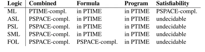
The complexities of these three model checking problems plus the satisfiability problem of the caustic sabotage logics are summarised in Table 1. The new sabo-tage operators strengthen standard modal logic on several (complexity) fronts.

• The satisfiability problems for SML, PSL and ASL are undecidable.

• The combined model checking problems for SML, PSL and ASL are all PSPACE-complete.

Interestingly, there is no difference in complexity between SML, PSL and ASL, even though, intuitively, this sentence lists them in order of decreasing expressive power.

1.2 Temporary Unavailability

This section proposes and motivates a newnon-caustic sabotage operation. The first and foremost reason for this proposal is architectural interest, but I admit that I initially hoped that it would fill the gap between standard modal logic and the caustic sabotage logics. It turns out to do so, but in a way I did not expect. More about this in §2.3. Consider the following scenarios.

Scenario 1. When dealing with computer networks like the Internet, there are al-ways connections that fail. But in general this is not because the computers or networks are physically destroyed by some malevolent force, but because of tem-porary failure. This means that broken entities might eventually be repaired, or might even automatically repair themselves. Furthermore, if failures are indepen-dent random events, it is very unlikely that many entities fail concurrently.

Scenario 2. A researcher is travelling toward an important conference. She is travelling by car and receives a radio message that there is a traffic jam ahead. If the jam is still some time ahead, then instead of rushing to the nearest train station to bypass the traffic jam, and arrive a little late for certain, she might take her chances and hope that the traffic jam will naturally resolve before she hits it.

(5)

1.3 Outline of the article 2 TUL

Note that, although we are using terminology from probability theory and tem-poral reasoning, we are not trying to model chance or time. We are just motivating the idea that compromised entities may eventually return to their normal state.

These scenarios suggest a differentnon-causticsabotage concept. The structure does not crumble as before, but certain parts become temporarily unavailable. We will restrict attention to the deletion of edges, as it is in a sense simpler (to remove a world from a model, one also has to remove all incident edges) and it allows efficient reuse of ideas from [Roh04].

1.3 Outline of the article

[image:5.595.117.478.452.544.2]

The next section, §2, treats the simplest instance of non-caustic sabotage, namely temporary removal of arbitrary single edges. This results in the Temporary Un-availability Logic. The complexity of TUL is subsequently analysed along the lines of [Roh04]. In section §3 we present and motivates a generalisation of TUL called General Modification Logic or GML. Where TUL deals with temporary re-moval of single edges, allowing any individual edge to be removed, GML abstracts away from the actual way in which the model is altered, and introduces restricted accessibility between different alterations. The actual underlying mechanism is a variation of product update (see [BMS98]). We conclude with a comparison of all treated sabotage logics and a list of open problems in §4.

Table 1 Complexities of standard problems for sabotage logics, standard modal logic and first order logic.

Logic Combined Formula Program Satisfiability

ML PTIME-compl. in PTIME in PTIME PSPACE-compl. ASL PSPACE-compl. in PTIME in PTIME undecidable PSL PSPACE-compl. in PTIME in PTIME undecidable SML PSPACE-compl. in PTIME in PTIME undecidable FOL PSPACE-compl. PSPACE-compl. in PTIME undecidable

2 Temporary Unavailability Logic (TUL)

(6)

2.1 Formalisation 2 TUL

2.1 Formalisation

Definition 2.1. Let Φ be a set of proposition letters. The language TUL is the smallest set of formulae containing all formulae generated by the the grammar

ϕ ::= > | p | ¬ϕ | ϕ1∨ϕ2 | ^ϕ | _^*ϕ (1)

The operator_^* is called thetemporary unavailabilityoperator. Analogous to the

dual operator, we define *ϕ := ¬_^*¬ϕ. The fragment of TUL that consists of *

^-free formulae is equivalent to the standard modal logic (ML).

Definition 2.2. LetObe a set of modal operators. Theoperator depthwith respect toO, is given by odO(ϕ) where

ϕ 7→ odO(ϕ)

> 7→ 0

p 7→ 0

¬ϕ 7→ odO(ϕ)

ϕ∨ψ 7→ max

odO(ϕ),odO(ψ)

4ϕ 7→

        

odO(ϕ)+1 if4 ∈O

odO(ϕ) otherwise

For a modal language with operator setO, we abbreviate odO(ϕ) to od(ϕ). The

modal language will always be clear from the context.

Definition 2.3. LetW be a non-empty set of worlds,R :W×W → _Nan acces-sibility multi-relation andV :Φ →

℘

(W) a valuation. We let amodelbe a tuple M=(WM,RM,VM) as usual.

Definition 2.4. Forw,v∈W, we writewRvand also (w,v)∈RforR(w,v)>0 and converselyw6RvforR(w,v)=0. Also|R|=P

w,v∈WR(w,v).

Definition 2.5. We define two multi-relation alteration operators,+and−, that add a unit to or remove a unit from the multiplicity of a certain edge. For (r,s),(t,u)∈

W×Wlet:

R+(r,s)(u,

v) =

        

R(u,v)+1 if (u,v)=(r,s)

R(u,v) otherwise (2)

R−(r,s)(u,

v) =

        

R(u,v)−1 if (u,v)=(r,s)

R(u,v) otherwise (3)

Note that the edge removal operator uses subtraction on the natural numbers, for which 0−x=0. This should not matter, as we do not intend to use the function in this case.

Remark2.6. (3) defines a right inverse of (2), for R+(r,s)

(7)

2.1 Formalisation 2 TUL

Definition 2.7. We now lift the multi-relation operators to models. Again for (r,s),(t,u)∈W×Wlet:

M+(r,s) = W,R+(r,s),V

(4)

M−(r,s) = W,R−(r,s),V

(5)

M(t,u)

(r,s) = M+(r,s)

−(t,u) (6)

Remark2.8. In (6), when (r,s)=(u,v) the model remains unaltered.

Definition 2.9. Now we can inductively define TUL formula satisfaction in a modelM, worldw∈Wand edge (r,s)∈W×W:

M,w,(r,s)> (7)

M,w,(r,s)p ⇔ w∈V(p) (8)

M,w,(r,s)¬ϕ ⇔ M,w,(r,s)1ϕ (9) M,w,(r,s)ϕ∨ψ ⇔ M,w,(r,s)ϕ or M,w,(r,s)ψ (10) M,w,(r,s)^ϕ ⇔ ∃v:wRv∧M,v,(r,s)ϕ (11) M,w,(r,s)_^*ϕ ⇔ ∃(t,u)∈R:M(t,u)

(r,s),w,(t,u)ϕ (12)

Definition 2.10. And finally we define formula satisfaction in a pointed model

M,w ϕ ⇔ ∃(r,s)∈R:M−(r,s),w,(r,s)ϕ (13) M,w∀ϕ ⇔ ∀(r,s)∈R:M−(r,s),w,(r,s)ϕ (14)

The choice for existential quantification as our primary definition is somewhat ar-bitrary, but it is in line with our preference for >, ∨, ^ over ⊥,∧,. There is some motivation for universal quantification too, especially when we want to rea-son about safety or security, that is, satisfaction irrespective of the first edge where disaster strikes.

Remark 2.11. Let M be a TUL model, w ∈ W and ϕ a TUL formula. During evaluation of M,w ϕ we need to evaluate certain subformulae of ϕin pointed models. Tracing the definitions given above, we see that in each nested evaluation N,v,(r,s) ψ, the actual model N equalsM−(r,s). We could have chosen an alternative definition of truth where we drag the original model along, like:

M−(r,s),w_^*ϕ ⇔ ∃(t,u)∈R:M−(t,u),wϕ (15)

(8)

2.2 Translation to First Order Logic 2 TUL

2.2 Translation to First Order Logic

Definition 2.12. LetM=(W,R,V) be a TUL model. We define its corresponding First Order Logic (FOL) structure

ˆ

M=(W,nPp| p∈Φ

o

,R)

wherePp=V(p).

Definition 2.13. Given a TUL formulaϕ, we inductively define itstranslation to FOLϕ(x,ˆ y,z). The variables x,y,z in the FOL formula are used to represent the rôle ofw,r,srespectively in the semantics of TUL.

ϕ 7→ ϕ(ˆ x,y,z)

> 7→ >

p 7→ Pp(x) ¬ϕ 7→ ¬ϕ(x,ˆ y,z)

ϕ∨ψ 7→ ϕ(ˆ x,y,z)∨ψ(x,ˆ y,z)

^ϕ 7→ ∃x0:xRx0∧ ¬(x=y∧x0 =z)∧ϕ(xˆ 0,y,z)

*

^ϕ 7→ ∃(y0,z0)∈R: ˆϕ(x,y0,z0)

Proposition 2.14. ϕ(x,ˆ y,z)is equivalent to a formula of FOL that uses only four variables.

Proof. It is well-known that the ML side of the translation can be done using only two variables. Note that the rule for_^* does not usey,zat all, so in particular does

not pass them on to the inductive application of the translation. Hence we can repeatedly reuse a single pairy0,z0for each (nested) occurrence of^.*

Remark2.15. The reduction of TUL to first order logic does not yield formulae in the Loosely Guarded Fragment, as discussed in [vB05b]. The culprits are the definition for^, in which the existential quantifier is not restrained by a conjunc-tion of atoms, and the definiconjunc-tion forwD, where the existential quantifier is properly restrained by a single atom, but the variablexdoes not co-occur in the atom with the existentially quantified variables.

Proposition 2.16. LetM=(W,R,V)be a TUL model. For all w,r,s,∈W we have M−(r,s),wϕ iff Mˆ ϕ(w,ˆ r,s)

Proof. By induction on the structure ofϕ. The only interesting cases are^and^.*

• The formula is of the form^ϕ. We need to show

M−(r,s),w^ϕ iff Mˆ ^cϕ(w,r,s)

that is

∃v:w R−(r,s)

v∧M−(r,s),vϕ iff

(9)

2.3 Model Checking Complexity 2 TUL

• The formula is of the form_^*ϕ. We need to show

M−(r,s),w_^*ϕ iff Mˆ ^c*ϕ(w,r,s)

Omitting the outer models and noting M−(r,s)(t,u)

(r,s)=M−(t,u) that is

∃(t,u)∈R:M−(t,u),wϕ iff ∃(y0,z0)∈R: ˆϕ(x,y0,z0) which also follows by the induction hypothesis and renaming of variables.

2.3 Model Checking Complexity

We turn to the problem of TUL model checking. We consider the instance of model checking where both the model and the formula are considered as input. Given a formulaϕ, modelMand worldw, how hard is it to determine whetherM,wϕ? The translation to FOL of the previous section places the problem in PSPACE, but we can do better:

Proposition 2.17. The complexity of TUL model checking is in PTIME.

Proof. Letϕbe a TUL formula and M = (W,R,V) a TUL model. First observe that

1. There are at most ϕ

subformulae ofϕ.

2. There are at most|W|2many submodels ofMwhere a single edge’s multi-plicity has been decremented by one.

We give a procedure for determining truth ofϕin all worlds ofMsimultaneously in Algorithm 1. It is a dynamic programming algorithm, that constructs a table of partial solutions which are subsequently reused to answer more complicated questions fast. The algorithm performs|ϕ| · |W|2· |W|evaluations, each requiring

|W|2lookups in the worst case (which occurs at subformulae with_^* as their main

operator). The initial setup in line 1 and final sweep in line 22 do not surpass this amount of work. We conclude that the total needed time is

O|ϕ| · |W|5 ∈ PT I ME |ϕ|,|M|

Corollary 2.18. Formula and program complexity for TUL model checking are in PTIME too.

Corollary 2.19. As TUL is an extension of ML, and ML model checking is PTIME complete (see Table 1), TUL model checking is PTIME complete as well.

(10)

2.3 Model Checking Complexity 2 TUL

Algorithm 1Dynamic programming algorithm for TUL model checking.

1: Constructϕ1, ϕ2, . . . , ϕn, a list of all subformulae of ϕ ordered by increasing

formula length. Obviouslyϕitself is the longest subformula, soϕn=ϕ.

2: Allocate a tableT of truth-values of sizen× |W|2× |W|. 3: for allϕido{the first dimension ofT}

4: for all(r,s)∈W×Wdo{the second dimension ofT} 5: for allw∈Wdo{the third dimension ofT}

6: ifϕi =>then

7: T[i,(r,s),w]=true

8: else ifϕi= pthen

9: T[i,(r,s),w]=V(p) 10: else ifϕi=¬ϕathen{a<i}

11: T[i,(r,s),w]=notT[a,(r,s),w] 12: else ifϕi=ϕa∨ϕbthen{a,b<i}

13: T[i,(r,s),w]=T[a,(r,s),w]orT[b,(r,s),w] 14: else ifϕi=^ϕathen{a<i}

15: T[i,(r,s),w]=1 iffthere is somevs.t.w(R−(r,s))vandT[a,(r,s),v] 16: else ifϕi=_^*ϕ_athen{a<i}

17: T[i,(r,s),w]=1 iffthere aret,u∈Ws.t.T[a,(t,u),w]

18: end if

19: end for

20: end for

21: end for

(11)

2.4 Satisfiability 3 GML

2.4 Satisfiability

TUL model checking can be done efficiently, as shown by the previous section, and in this respect TUL resembles standard ML. This similarity does not extend further, as shown by the following results. Multi-agent TUL extends TUL by including a sabotage modality for several agents.

Proposition 2.20. Multi-agent TUL does not have the finite model property:

Proof. The argument in [Roh04, definition ofϕ∞ on p63] carries over to

multi-agent TUL, for it uses only singly nested occurrences of the global sabotage

oper-ator.

Proposition 2.21. The satisfiability problem for multi-agent TUL is undecidable.

Proof. The argument in [Roh04, section 3.3] that reduces Post’s correspondence problem to SML using only singly nested global sabotage operators carries over to

TUL.

2.5 Several Considerations

The following points require some attention.

• In the introduction we talked about temporarily unavailable entities that will eventually be restored. The current semantics allows the case that a certain single edge remains unavailable for the entire evaluation of the formula. One could add afairnesscondition, which states that each nested evaluation of the_^* operator must take out a different edge.

• One could consider the ability to remove several edges. This requires an edge buffer together with an edge replacement protocol. We could think of for example the bag, queue or stack of fixed size. This allows the model to be altered in a more intricate fashion, while still allowing for the eventual return of removed edges.

• One could desire the ability to remove worlds. We have restricted ourself to edge removal, but we can model deleting a world by simultaneously sup-pressing all incident edges. We call this operationblackout.

These points are the motivation for the generalisation of TUL to GML in the next section.

3 General Modification Logic (GML)

(12)

3.1 Modification frames 3 GML

3.1 Modification frames

LetFbe the class of Kripke frames.

Definition 3.1. A function1i: F→ Fis called amodification frame generatorif for allF = (W,R) ∈ _Fthere are a set F, a directed graphE ⊆ F×F overF and directed multi-graphsRf ⊆W×WoverWfor all f ∈F, such that

i(F)=

F,E,n

Rf

o

f∈F

.

We lift i from frames to models thus: i(M) = i(W,R). We call the structure i(M) =

F,E,n

Rf

o

f∈F

themodification framegenerated byifromMand denote it byTwhen iandMare unambiguous. Furthermore, we call the elements of F modifications. We regard them as names for operations onR, and for each f ∈ F we say thatRf is theresultof f.

Example 3.2. For TUL, we can specify the corresponding modification frame gen-eratoriT U Las follows

iT U L(W,R) =

F,E,n

Rf

o

f∈F

(17)

F = (a,

b)|aRb (18)

E = F×F (19)

R(a,b) = R−(a,b) (20)

We take as modificationsFall edges in the source frame (flattened from a multi-graph to a normal multi-graph). The inter-modification accessibility multi-graphEis the com-plete graph overF, and the resultRf (an accessibility relation overW) that

corre-sponds to f is obtained by removing the edge f fromR.

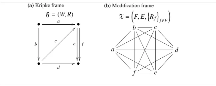
Example 3.3. Consider the Kripke frameFin Figure 0a. Application ofiT U L to

this frame yields the modification frameTin Figure 0b. Each modification f ∈ F (node of T) corresponds to an edge of F. The accessibility relation E between modifications is the complete graph, as shown by the undirected arcs. Reflexive arcs are omitted from the figure for brevity.

3.2 Logic

Now that we have defined the structures of interest, we turn to the logic.

Definition 3.4. Let Φ be a set of proposition letters. The language of General Modification Logic (GML) is the smallest set of formulae containing all formulae generated by the the grammar

ϕ ::= > | p | ¬ϕ | ϕ1∨ϕ2 | ^ϕ | ^?ϕ (21)

1_Technically,_i_{is a class function. In particular, it is a formula in the language of set theory.}

(13)

[image:13.595.117.477.151.294.2]

3.2 Logic 3 GML

Figure 1Example (a) source frame and (b) modification frame generated byiT U L.

(a)Kripke frame F=(W,R)

• a //

b • f e •

d //

c ? ? •

(b)Modification frame

T=

F,E,n

Rf

o

f∈F

b .. .. .. .. .. .. .. . N N N N N N N N N N N N N N c = = = = = = = = a p p p p p p p p p p p p p p N N N N N N N N N N N N N N = = = = = = = = d f p p p p p p p p p p p p p p _e

The operator_^? _{is called the}_{modification operator. Analogous to}_{, the dual} oper-ator of^, we define?ϕ := ¬^?¬ϕ. The fragment of GML that consists of^?-free formulae is equivalent to the standard modal logic (ML).

Definition 3.5. The semantics of GML are defined relative to a modification frame generatorithat we consider fixed to avoid subscripts. Fix a modelM= (W,R,V), and letT = i(M). Additionally fix a world w ∈ W and a modification f ∈ F. Furthermore fix a GML formula ϕ. We inductively define truth in the pointed model, pointed frame combinationM,w,T, f by

M,w,T,f > (22)

M,w,T,f p ⇔ w∈V(p) (23)

M,w,T,f ¬ϕ ⇔ M,w,T,f ₁ϕ (24) M,w,T,f ϕ∨ψ ⇔ M,w,T,f ϕ or M,w,T,f ψ (25) M,w,T,f ^ϕ ⇔ ∃v∈W :wRfv∧M,v,T,f ϕ (26)

M,w,T,f _^*ϕ ⇔ ∃g∈E: f Eg∧M,w,T,gϕ (27)

We callwthefirst focusorcurrent worldand f thesecond focusorcurrent mod-ification. (22) – (25) are just propositional logic with additional ballast. (26), defining the GML diamond operator, is similar to the corresponding clause in stan-dard ML, but readswRfv instead ofwRv. This ensures that the first focus only

uses edges that exist inRf, the result of the current modification. (27), defining

the GML modification operator, allows the second focus to make transitions inE, independent of the current world. Hence the GML modification operator behaves as a regular diamond in the modification frame.

(14)

3.3 Game 3 GML

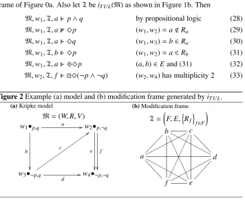
frame of Figure 0a. Also letTbeiT U L(M) as shown in Figure 1b. Then

M,w1,T,ap∧q by propositional logic (28)

M,w1,T,a1^p (w1,w2)=a<Ra (29)

M,w₁,T,a_^q (w1,w3)=b∈Ra (30)

M,w1,T,b^p (w1,w2)=a∈Rb (31)

M,w1,T,a_^^* p (a,b)∈Eand (31) (32)

[image:14.595.123.480.129.424.2]

M,w2,T, f ^(* ¬p∧ ¬q) (w₂,w₄) has multiplicity 2 (33)

Figure 2Example (a) model and (b) modification frame generated byiT U L.

(a)Kripke model

M=(W,R,V) w1•p,q a //

b

w2•p,¬q

f e

w₃•¬p,q

d // c : : v v v v v v v v v v v v v v v v v v v

w₄•¬p,¬q

(b)Modification frame

T=

F,E,n

Rf

o

f∈F

b .. .. .. .. .. .. .. . N N N N N N N N N N N N N N c = = = = = = = = a p p p p p p p p p p p p p p N N N N N N N N N N N N N N = = = = = = = = d f p p p p p p p p p p p p p p _e 3.3 Game

These semantics can easily be interpreted as a two player formula game. The game starts with a GML formulaϕ, a Kripke modelM = (W,R,V) called theoriginal model, a worldw, a modification frameTand a modification f. The players are called Verifier and Falsifier, and they try to do toϕwhat their name suggests. We call (W,Rf,V) thecurrent model. The player to move is determined by the structure

of the formula:

• >. Verifier wins.

• ¬ϕ. Players exchange roles, the game continues with the formulaϕ.

• ϕ∨ψ. Verifier picks one ofϕ,ψto continue the game.

• _^ϕ. Verifier makes a move (w,v) in the current model. The game continues with the formulaϕand worldv.

• _^*ϕ. Verifier makes a move (f,g) in the modification frame. The game

con-tinues with the formulaϕ and the modification g, hence with new current model (W,Rg,V).

Proposition 3.7. Verifier has a winning strategy iffM,w,T,f ϕ.

(15)

3.4 Modification Product 3 GML

3.4 Modification Product

As pointed out in §3.2, the modal operators of GML are similar to the standard diamond operator. This section describes an operation called modification product, that maps a model and corresponding modification frame to a new structure, in which standard bi-agent modal logic suffices.

Definition 3.8. Starting from a Kripke modelM=(W,R,V) and the modification frameT= i(M) =

F,E,n

Rf

o

f∈F

generated byifromMwe define the modifica-tion productby

M×T=W×F,RM₁×T,RM₂×T,VM×T (34) where

(w,f)∈VM×T(p) ⇔ w∈V(p) (35) (w,f)RM₁×T(v,g) ⇔ f =g∧wRfv (36)

(w,f)RM₂×T(v,g) ⇔ w=v∧ f Eg (37)

Definition 3.9. For f ∈F, we call the restriction of the modification productM×T to worlds inW×

f themodification imageof f. The only possible accessibility arrows for the second agent within the accessibility image offare reflexive arrows, and these are present iff f E f.

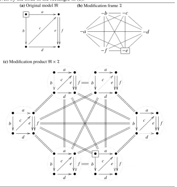
The idea behind these definitions is this: the modification frame specifies a set of modifications. To form the modification product, we “apply” each modifica-tion to the original model and concatenate the resulting modificamodifica-tion images. The accessibility relation for the first agent is determined by the result of each modifica-tion, and relates different worlds within the same modification image. On the other hand, the accessibility relation for the second agent relates images of the same original world between different modification images, for those modifications that are related in the modification frame. The valuations do not consider edges at all, and they are just replicated in each modification image.

Example 3.10. We have shown a particular model and its TUL modification frame in Figure 2. The corresponding modification product is shown in Figure 3. To emphasise the accessibility relation, this figure omits the valuations. The valuation in the product model is formed by repeating copies of the valuation of the source model.

3.5 Reduction to ML-2

We reduce GML to ML-2, bi-agent standard modal logic.

(16)

[image:16.595.124.481.282.659.2]

3.5 Reduction to ML-2 3 GML

Figure 3Modification product construction. In (c), the individual modification im-ages are enclosed by dotted circles, and the removed edge within each modification image is shown as a dotted arrow. Double edges between modification images of f andgabbreviate that (w,f) and (w,g) are related for allw∈W. As an example, when the current world and current modification are given by the nodes in rectan-gles in (a) and (b), then the resulting current world in the modification product is given by the node in the rectangle in (c).

(a)Original modelM

• a //

b • f e •

d //

c ? ? •

(b)Modification frameT

−b 11 11 11 11 11 11 11 1 Q Q Q Q Q Q Q Q Q Q Q Q Q Q

Q −c

C C C C C C C C −a { { { { { { { { m m m m m m m m m m m m m m m Q Q Q Q Q Q Q Q Q Q Q Q Q Q Q B B B B B B B

B −d

(c)Modification productM×T

•

a //

b

•

f e

•

a //

b

•

f e

•

d //

c??

•

d //

c ??

•

a //

b

•

f e

•

a //

b

•

f e

•

d //

c ??

•

d //

c ??

•

a //

b

•

f e

•

a //

b

•

f e

•

d //

c??

•

d //

c??

•

o o o o o o o o o o o o o o o o o o o o o o o o o o o o o o o o o o o o o o o o O O O O O O O O O O O O O O O O O O O O O O O O O O O O O O O O O O O O O O O O @ @ @ @ @ @ @ @ @ @ @ @ @ @ @ @ @ @ O O O O O O O O O O O O O O O O O O O O O O O O O O O O O O O O O O O O O O O O // // // // // // // // // // // // // // // // // // // // @ @ @ @ @ @ @ @ @ @ @ @ @ @ @ @ @ @

ooooooooo

ooooooooo oo

oooooo

(17)

3.5 Reduction to ML-2 3 GML

by

ϕ 7→ ϕˇ

> 7→ >

p 7→ p

¬ϕ 7→ ¬ϕˇ ϕ∨ψ 7→ ϕˇ ∨ψˇ

^ϕ 7→ ^1ϕˇ

?

^ϕ 7→ ^2ϕˇ

Proposition 3.12. The reduction preserves truth, in other words

M,w,T,f ϕ ⇔ M×T,(w, f)ϕˇ (38) Proof. By induction on the complexity ofϕ, and case distinction on structure

• ϕ=>,ϕ=¬ψ,ϕ=ϕ₁∨ϕ₂are all trivial.

• ϕ= p. We need to show

M,w,T,f p ⇔ M×T,(w,f)p (39) which both are equivalent tow∈V(p).

• ϕ=^ψ. We need to show

M,w,T, f _^ψ ⇔ M×T,(w, f)^1ψˇ (40)

well

M×T,(w,f)^1ψˇ (41)

⇔ ∃(v,g) : (w, f)RM₁×T(v,g)∧M×T,(v,g)ψˇ (42)

⇔ ∃v:wRfv∧M×T,(v,f)ψˇ (43)

⇔

IH ∃v:wR_fv∧M,v,T, f ψ (44)

⇔ M,w,T,f _^ψ (45)

• ϕ=_^?ψ. We need to show

M,w,T, f _^?ψ _⇔ _M_×_T,(w, _f₎_^₂ψˇ ₍₄₆₎ well

M×T,(w,f)^2ψˇ (47)

⇔ ∃(v,g) : (w, f)RM₂×T(v,g)∧M×T,(v,g)ψˇ (48)

⇔ ∃g: f Eg∧M×T,(w,g)ψˇ (49)

⇔

IH ∃g: f Eg∧M,w,T,gψ (50)

⇔ M,w,T,f _^?ψ ₍₅₁₎

(18)

3.6 Satisfiability 3 GML

3.6 Satisfiability

We saw that TUL, the simplest non-caustic sabotage logic, can be reduced to GML, from which it follows that the satisfiability problem for GML is generally undecid-able.2 One may think that this is in contradiction with the foregoing reduction of GML to ML, as the satisfiability problem for ML is certainly decidable! The prob-lem with this reasoning is of course that most ML models are not images of GML models under the above reduction.

3.7 Model Checking Complexity

We already saw that model checking for TUL is in PTIME. This means that for certain classes of modification frame generators, the model checking problem for GML is in PTIME as well. We can generalise this result by imposing a polynomial bound on the size of the modification frame, and this will place combined formula complexity for GML in PTIME in this case.

Proposition 3.13. Let i be a modification frame generator, and let there be an algorithm that for all finite F = (W,R) computes i(F) in time O(|W|n) for some fixed n. (This implies that |F| ∈ O(|W|n).) Then the combined model checking problem for i-GML is in PTIME.

Proof. LetM = (W,R,V) be a Kripke model, ϕa GML formula. We first com-puteT = i(M), which we can do in time polynomial in|M| by assumption. We proceed by computing the modification productM×T, which we can do in time polynomial in|M|, yielding a bi-agent Kripke model of polynomial size in|M|. We then compute ˇϕ, in time linear in

ϕ

. We finish by applying the model checking

algorithm for standard modal logic, which runs in polynomial time in both model and formula size. Hence the entire procedure can be completed in polynomial time in|M|and

ϕ

.

Remark3.14. This is a generalisation of Proposition 2.17.

3.8 Applications

We demonstrate the expressive power of GML by modelling the sabotage operators that we described in section §2.5, which lists possible extensions of TUL.

Fairness By takingE irreflexive, we get a fair sabotage operator. Evaluation of the sabotage operator requires making a move, picking an accessible modification, in the modification frame. When the accessibility relationEis irreflexive, we are forced to choose adifferentmodification.

(19)

3.8 Applications 3 GML

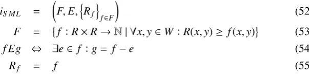
SML By takingFto contain any subrelation ofRand f Egiffgcontains a single edge less than f, we get the global sabotage modality of [Roh04]. Note that we identify modifications and results in this case.

iS ML =

F,E,n

Rf

o

f∈F

(52)

F =

f :R×R→_N| ∀x,y∈W :R(x,y)≥ f(x,y) (53)

f Eg ⇔ ∃e∈ f :g= f −e (54)

Rf = f (55)

This does not imply that we can do SML model checking in PTIME, for the set of modifications is exponentially large inM.

ASL We can not model adjacent sabotage, for the accessibility relation between modifications is not uniform, but in fact depends upon the focus of evaluation.

PSL To model path sabotage, we must make F even larger, including a modifi-cation for every subrelation ofRlike for SML, but now also labelling them with the current path deletion focus.

iPS L =

F,E,n

Rf

o

f∈F

(56)

F = W×

f :R×R→_N| ∀x,y∈W:R(x,y)≥ f(x,y) (57) (w,f)E(v,g) ⇔ w f v∧g= f −(w,v) (58)

R(w,f) = f (59)

Two modifications (w,f) and (v,g) are related if the edge (w,v) is present in f, and gis the result of deleting this edge from f.

Blackout The blackout operator simultaneously removes all edges incident to a certain world. It is used to model removing worlds in terms of edge deletions.

iBO =

F,E,n

Rf

o

f∈F

(60)

F = W (61)

E = F×F (62)

[image:19.595.170.472.178.250.2]

uRwv ⇔ uRv∧w,v (63)

Figure 4 shows an application of the fair blackout operator to the Idol model.

Protocols for multiple edge removal Given an algebraic specification S of a collection (say a bag, queue or stack), we take the modifications to be the states in the external behaviour ofS (see [Fok00]). We then takeRf to be Rminus all

(20)

[image:20.595.114.481.214.615.2]

3.8 Applications 3 GML

Figure 4Example of the fair blackout operator.

(a)Original (Idol) model M

• a //

b • f e •

d //

c ? ? •

(b)Modification frameT

− {}_O_O oo //

c c # # G G G G G G G G G G G G G G G G G

G − {a,OO c}

− {b}{{oo //

; ; w w w w w w w w w w w w w w w w w w w

−d,e,

f

(c)Modification productM×T

•

a

/

b

•

f

e

•

a

/

b

•

f

e

•

d

/

c

?

•

d

/

c

?

•

a

/

b

•

f

e

•

a

/

b

•

f

e

•

d

/

c

?

•

d

/

c

?

• k

s

+

3 K

S

[

c

#

?

;

C

{

K

S

k

(21)

4 CONCLUSION

4 Conclusion

We introduced and motivated TUL, a new sabotage modal logic. It lies in between ML and SML, for its model checking complexity is PTIME complete (like ML), but its satisfiability problem is undecidable (like SML).

We then generalised TUL and arrived at GML, which uses a modification frame generator to merge a Kripke model that represents the common starting point and a modification frame; an accessibility graph over modifications. We introduced mod-ification frame generators to construct modmod-ification frames for arbitrary frames. We reduced GML to bi-agent standard modal logic, and proved that its model checking problem is PTIME complete under certain conditions on the modifica-tion frame generator.

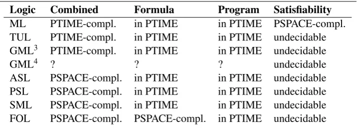
[image:21.595.119.478.326.463.2]

Table 2 summarises the results of this paper, and puts them into context.

Table 2Complexities of standard problems for sabotage logics and first order logic.

Logic Combined Formula Program Satisfiability

ML PTIME-compl. in PTIME in PTIME PSPACE-compl. TUL PTIME-compl. in PTIME in PTIME undecidable GML3 PTIME-compl. in PTIME in PTIME undecidable

GML4 ? ? ? undecidable

ASL PSPACE-compl. in PTIME in PTIME undecidable PSL PSPACE-compl. in PTIME in PTIME undecidable SML PSPACE-compl. in PTIME in PTIME undecidable FOL PSPACE-compl. PSPACE-compl. in PTIME undecidable

4.1 Open questions

The following interesting questions have remained unanswered:

• Under which conditions on the modification frame (generator) is the satisfi-ability problem of GML decidable? When F is a singleton set and E = ∅

we are working in standard modal logic, for which the satisfiability problem is decidable. When imodels temporary unavailability of single edges, we already enter the realm of undecidability.

• A somewhat related question is that of the finite model property. Which modification frame generators do have this property?

• Which modification frame generators have bisimulation invariance? [Roh04, p62] shows that global sabotage allows us to distinguish between loops and paths of otherwise indistinguishable worlds, thus losing bisimulation invari-ance.

(22)

4.2 Acknowledgements REFERENCES

4.2 Acknowledgements

The author would like to thank Prof. Dr. Johan van Benthem for his comments. He also appreciated the remarks by Drs. Steven de Rooij, correcting grammar, style and punctuation.

References

[BdRV01] Patrick Blackburn, Maarten de Rijke, and Yde Venema. Modal Logic. Cambridge University Press, 2001.

[BMS98] Alexandru Baltag, Lawrence S. Moss, and Slawomir Solecki. The logic of public announcements, common knowledge, and private suspicions. InTARK ’98: Proceedings of the 7th conference on Theoretical aspects of rationality and knowledge, pages 43–56, San Francisco, CA, USA, 1998. Morgan Kaufmann Publishers Inc.

[Fok00] Wan Fokkink. Introduction to Process Algebra. Springer, 2000.

[Roh04] Philipp Rohde. On Games and Logics over Dynamically Chang-ing Structures. PhD thesis, Rheinisch-Westfälischen Technischen Hochschule Aachen, 2004.

[vB05a] Johan van Benthem. An essay on sabotage and obstruction, essays in honor of Jörg Siekmann on the occasion of his 69th birthday. In D. Hutter, editor,Mechanizing Mathematical Reasoning, pages 268– 276. Springer Verlag, 2005.

PP 2008 10: Temporary Unavailability Logic and General Modification Logic

Temporary Unavailability Logic

and General Modification Logic

Contents

1

Introduction

2

Temporary Unavailability Logic (TUL)

℘

3

General Modification Logic (GML)

•

•

•

•

•

•

•

•

•

•

•

•

•

•

•

•

•

•

•

•

•

•

•

•

•

/

/

•

•

/

/

•

•

/

/







?

?









•

•

/

/

?

?

•

•

/

/

•

•

/

/

•

•

/

/







?

?



