Climate forcing and sudden change in marine ecosystems

Climate Forcing and Sudden Change

in Marine Ecosystems

by

Michael Andrew Litzow, B.S., M.S.

Institute for Marine and Antarctic Studies

Submitted in fulfillment of the requirements for the Doctor of Philosophy degree

Declaration of Originality

This thesis contains no material which has been accepted for a degree or diploma by

the University or any other institution, except by way of background information and

duly acknowledged in the thesis, and to the best of my knowledge and belief no

material previously published or written by another person except where due

acknowledgement is made in the text of the thesis, nor does the thesis contain any

material that infringes copyright.

Signed: _________________________

Date: ______________

Michael Litzow

Authority of Access

Statement of Co-Authorship

The following people and institutions contributed to the publication of work

undertaken as part of this thesis:

Candidate:

Michael Litzow, Institute for Marine and Antarctic Studies

Author 1:

Franz Mueter, University of Alaska, Fairbanks, USA

Author 2:

Alistair Hobday, Commonwealth Scientific and Industrial Research

Organization

Author 3:

Dan Urban, National Oceanic and Atmospheric Administration, USA

Author 4:

Stewart Frusher, Institute for Marine and Antarctic Studies

Author 5:

Peter Daan, Phillip Island Nature Parks

Author 6:

Geoffrey Tuck,

Commonwealth Scientific and Industrial Research

Organization

Paper 1: Reassessing regime shifts in the North Pacific: incremental climate

change and commercial fishing are necessary for explaining decadal-scale

biological variability.

Global Change Biology, 20, 38-50.

Located in Chapter 1

Candidate was the primary author and had the idea for the study. Authors 1 and 2

contributed to study design, analysis and write-up.

Paper 2: Assessing the ecological importance of climate regime shifts: an

approach from the North Pacific Ocean.

Progress in Oceanography, 120, 110-119.

Located in Chapter 2

Candidate was the primary author and had the idea for the study. Author 1

contributed to study design, analysis and write-up.

Paper 3: State-dependent climate effects on community assemblages in Alaskan

marine ecosystems.

Submitted to Marine Ecology Progress Series.

Located in Chapter 3

Candidate was the sole author on this paper.

Paper 4: Rising catch variability preceded historical fisheries collapses in Alaska.

Ecological Applications, 23, 1475-1487.

Located in Chapter 4

Candidate was the primary author and had the idea for the study. Authors 1 and 3

contributed to study design, analysis and write-up.

Paper 5: Detecting complex ecological change in data-limited situations: an

example from southeast Australia.

Submitted to Regional Environmental Change.

Located in Chapter 5

We the undersigned agree with the above stated “proportion of work undertaken” for

each of the above published (or submitted) peer-reviewed manuscripts contributing to

this thesis:

Signed: __________________

______________________

Stewart Frusher

Mike Coffin

Supervisor

Executive Director

Institute for Marine and

Institute for Marine and

Antarctic Studies

Antarctic Studies

University of Tasmania

University of Tasmania

Our traditional view of natural systems, therefore, might well be less a

meaningful reality than a perceptual convenience.

Table of Contents

Acknowledgements...xiv

Abstract...1

Introduction...5

Chapter 1 Reassessing regime shifts in the North Pacific: incremental climate

change and commercial fishing are necessary for explaining decadal-scale

biological variability ...11

Abstract ...12

Introduction ...13

Materials and Methods ...15

Data...15

Analysis ...18

Results ...21

Goal 1...21

Goal 2...22

Goal 3...25

Discussion...25

Supporting Information...31

Chapter 2 Assessing the ecological importance of climate regime shifts: an

approach from the North Pacific Ocean ...41

Abstract ...42

Introduction ...44

Materials and methods ...47

Data...47

Analysis ...49

Results ...53

Leading axes of ecological variability ...53

Abrupt vs. gradual models of variability ...57

PDO behavior as a measure of ecosystem forcing ...57

Assessing the putative 2007/08 climate shift...57

Discussion...60

Supporting Information...65

Chapter 3 The PDO-NPGO transition produces non-additive community

control in two North Pacific ecosystems ...79

Abstract ...80

Introduction ...81

Methods ...83

Results ...88

Discussion...92

Supplemental Information ...96

Chapter 4 Rising catch variability preceded historical fisheries collapses in

Alaska...101

Abstract ...102

Introduction ...103

Materials and Methods ...105

Data...105

Analysis ...109

H1: Spatial variability in catch increases prior to population collapse ...112

H2: Spatial skewness in catch increases prior to population collapse...113

H3: Increased variability is a transient phenomenon associated with collapse...114

Discussion...114

Chapter 5 Detecting complex ecological change in data-limited situations: an

example from southeast Australia ...123

Abstract ...124

Introduction ...125

Materials and Methods ...126

Terminology...126

Data...127

Analysis ...129

Results ...135

PCA results ...135

Biological change ...137

Climate-biology covariation ...138

Discussion...139

Synthesis...147

Conclusions and Recommendations ...147

Future Directions ...150

List of Figures

Fig. 1.1 Approximate locations for 36 biological time series included in analysis. Dashed line indicates spatial extent of SST and SLP data used in PCA of regional climate. ...15

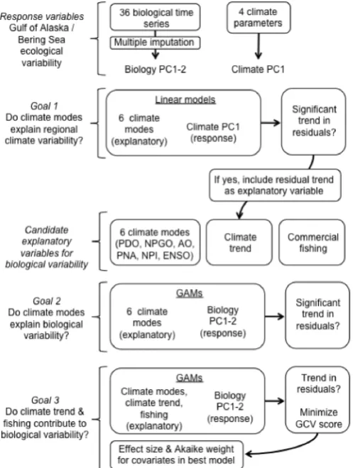
Fig. 1.2 Schematic of analytical steps used in the study. ... 17

Fig. 1.3 Inability of large-scale climate modes to explain regional climate variability: observed values of climate PC1, and residual values from linear model invoking full set of climate modes (PDO, NPGO, AO, PNA, NPI, MEI lag1). Significant linear trend in model residuals (P = 0.03) indicates that the model fails to capture a directional trend in regional climate, and therefore violates the assumption of independent residuals...21

Fig. 1.4 Strongest loadings (absolute value ≥ 0.2) for (a) biology PC1 and (b) biology PC2. Complete loadings are presented in Table 1.S5. G = Gulf of Alaska, S = Southeast Alaska (part of the Gulf of Alaska ecosystem), B = Bering Sea.. ...22

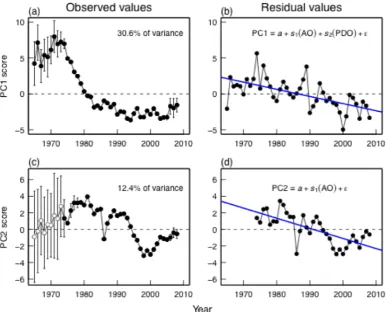
Fig. 1.5 Inability of internal climate variability to explain regional biological variability: time series of observed scores for biology PC1 and PC2 (a, c), and residual scores from best GAMs that could be constructed from internal climate modes alone (b, d). Observed values are mean ± 2 SD from the final 100 imputations used to estimate missing values in individual biology time series (see Methods for details). Years without error bars contained no missing values. Open circles in (c) indicate years where SD of estimated PC2 was greater than the absolute value of mean estimated scores across the time series; these years were not used in subsequent analysis. Plotted residuals from best GAMs invoking only internal climate modes (b, d) show linear trends (heavy lines) that were significant in both cases (PC1: P = 0.001; PC2: P = 0.002), indicating that the models failed to explain directional trends in community variability, and therefore violated the assumption of independent residuals.. ...23

Fig. 1.6 External forcing of leading axes of community-level biological variability. Partial residual plots from best GAM for biology PC1 (a-e) and biology PC2 (g-k) that could be constructed when invoking the full set of forcing variables (internal climate modes, residual climate trend and commercial catch). Solid lines indicate predicted effects with other variables held constant at their mean, dashed lines = 95% CI. Text in each panel indicates effect size in model (proportion of deviance uniquely explained by each covariate). Akaike weights for each variable included in best model for biology PC1 (f) and biology PC2 (l), summed across the global set of candidate models for each PC. Catch = commercial catch, CT = climate trend.. ... 27

Fig. 1.S1 Time series of external forcing variables used in analysis of community variability, scaled as 0 mean, unit variance. Time series that were smoothed for analysis show both smoothed data (black) and raw data (gray)...39

Fig. 2.1 Approximate location of time series used in analysis. Locations for large-scale climate indices not indicated... 48

press disturbance), while the 1988/89 event is characterized by less stable post-shift conditions (weak press disturbance). ...52

Fig. 2.3 Leading modes of ecological variability in the northeast Pacific Ocean: strongest PCA loadings for (a) large-scale climate indices; (b, c) local climate parameters; (d, e) biology time series.. ...54

Fig. 2.4 Leading modes of ecological variability in the northeast Pacific Ocean: PCA time series. Blue circles indicate observations, red lines indicate best models for temporal variability: threshold (STARS/ANOVA; a-c, e), or gradual (GAM, d), as determined by AIC. Error bars = 95% CI, and reflect uncertainty associated with estimating missing values. Dashed black vertical line indicates simultaneous changes in 1976/77, dashed grey vertical line indicates 2007/08. . ...56

Fig. 2.5 Patterns and consequences of changing behavior in the PDO: time series of PDO amplitude (mean absolute value) and strength of PC1biol (average Pearson's |r| between individual time series and PC score). Both time series calculated on a 15-year sliding window to match the length of L in STARS analysis, and standardized as mean 0, unit variance. ... 57

Fig. 2.6 Year-to-year changes in leading axes of northeast Pacific biological variability: Each year plots total change in PC1biol-PC2biol phase space from previous year. Error bars = 95% CI, indicating uncertainty from estimating missing time series variables. The 2007/08 change was 311% of the mean across all other years in the time series (z = 5.53, P < 0.00001). ...58

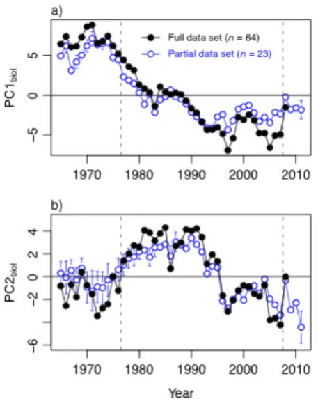
Fig. 2.7 Assessing the persistence of post-2007/08 change in (a) PC1biol, and (b) PC2biol, using a partial set of biology time series that could be updated at least through 2010. Error bars for PC scores calculated from partial data sets = 95% CI, and reflect uncertainty associated with estimating missing values. Time series for PC scores from full data set are plotted for comparison, with error bars omitted for clarity. Dashed vertical lines indicate 1976/77 climate regime shift and putative 2007/08 shift. STARS failed to detect a shift following 2007/08 for either PC time series calculated from the partial data set (P' > 0.2). ... 59

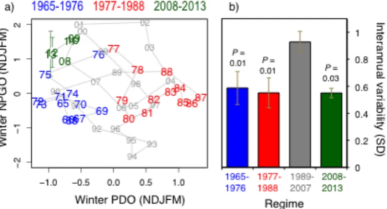
Fig. 2.8 Variability in the PDO and NPGO across 2007/08, relative to historical shifts. (a) NPGO-PDO phase space. Data are smoothed with a 3-year running mean to isolate the trend from noise, except for 2013, which is a 2-year running mean. Colors group earlier climate regimes (1966-1976 and 1977-1988) and recent years (2008-2013). Error bars = 95% CI, and reflect uncertainty associated with estimating 2013 NPGO value. (b) Press perturbations for four possible PDO-NPGO regimes: average SD calculated for every 5-year window in each regime, error bars = 95% CI. Note that lower SD values indicate a stronger press disturbance. Plotted P-values are pairwise comparisons with 1989-2007 variability, derived from randomized ANOVA. ... 60

Fig. 3.1 (a) Approximate location of 36 population time series used in analysis. (b) Time series showing strongest loadings (absolute value ≥ 0.2) on biology PC1. (c) Time series showing strongest loadings on biology PC2. B = Bering Sea, G = Gulf of Alaska, S = southeast Alaska (part of the Gulf of Alaska). Redrawn from Litzow et al. (2014)..

...84

forcing, corresponding to threshold generalized additive model (TGAM). Redrawn from Scheffer et al. (2001)... 86

Fig. 3.3 Changes in the relative importance of the PDO and NPGO across the 1988/89 climate transition. (a) Amplitude (average absolute value) of the winter (NDJFM) PDO and NPGO indices, 1965-2008. Data smoothed with 11-year running mean and normalized as zero mean, unit variance for the period plotted. (b) Relative importance (LMG scores/partial R2 values) for PDO and NPGO in linear regression of regional climate PC1 scores. Loadings for regional climate PCA in Table 3.1. ...89

Fig. 3.4 Non-additive control of biology PC1 scores, 1965-2008: relationship with (a) the winter (NDJFM) PDO, and (b) the winter (JFM) NAM. Both climate indices smoothed with 3-year running mean prior to plotting. Filled symbols indicate years included in best models of PC1 response to external forcing (GAM for 1965-1977, TGAM for 1978-2008). Error bars ± 2SD, indicating uncertainty associated with estimating missing values.. ... 90

Fig. 3.5 Non-additive control of biology PC2 scores, 1973-2008: relationship with (a) commercial catch lagged 3 years, (b) the regional climate trend, independent of natural modes of climate variability, and c) the winter (NDJFM) NPGO. Filled symbols indicate years included in best model (TGAM) of PC2 response to forcing. Climate trend and NPGO smoothed with 3-year running mean prior to plotting. Error bars ± 2SD, indicating uncertainty associated with estimating missing values...92

Fig. 3.6 Prediction skill for statistical models of climate-biology covariation across examples of continuous (1976/77) and non-additive (1988/89) forcing-response relationships. (a) Prediction skill for models of variability in biology PC1 scores. (b) Prediction skill for models of Bering Sea sockeye salmon catch, log transformed and lagged 2 years to reflect year of ocean entry. Models are GAMs invoking the PDO for observation periods of different lengths (9-11 years), ending 1-4 years before shifts. Mixed-effects models showed that root mean squared prediction error averaged across all models was significantly greater for non-additive forcing than for continuous forcing, both for PC1 (t16 = 5.47, P = 0.0001), and for Bering Sea sockeye salmon catches (t16 = 25.29, P < 0.0001). ... 93

Fig. 4.1 Approximate location of fisheries included in study. . ...105

Fig. 4.2 (A) Catch time series included in study, plotted relative to maximum catch size for each fishery. Collapse points used in analysis are indicated by vertical dashed lines. Note that Bristol Bay red king crab data were separated into collapsing and non-collapsing periods for analysis. (B) Sample size (number of active statistical areas) by fishery and year. Horizontal dashed lines indicate mean n for each fishery. Missing years within time series were either years of identified collapse, which were not used in analysis, or years with zero catch for the fishery. ... 108

Fig. 4.4 (A) Length of potential warning from rising spatial variability: estimates of trend in SDL (slope on year) across all collapsing fisheries for analysis periods ending 1-5 years prior to collapse. Sample sizes (number of fisheries with n ≥ 10 years of data for different analysis periods) at top of panel. Random-effects models showed significant increases in variability, across all fisheries, for data ending 1-4 years prior to collapse (one-tailed P ≤ 0.02). (B) "False positives" test: estimates of trend in variability across all collapsing and non-collapsing fisheries (random-effects model, one-tailed P = 0.04). All error bars = 95% CI. . ... 112

Fig. 4.5 Trends in spatial skewness of catch across all fisheries: partial residual plots after effects of sample size have been accounted for. Lines illustrate best-fit linear trends, with associated one-tailed P-values testing hypothesis of increasing skewness prior to collapse. Trends are indicated for non-collapsing fisheries, but P-values are not plotted as these fisheries were not included in hypothesis test for pre-collapse behavior. Random-effects model showed no evidence of pre-collapse increases in skewness across all collapsing fisheries (one-tailed P = 0.83). ... 115

Fig. 4.6 Evidence of persistent increases in spatial variability in post-collapse fisheries, relative to pre-collapse state (ANCOVA, pre- vs. post-collapse state, P < 0.0001). Error bars = 95% CI.. ...116

Fig. 5.1 Schematic depicting steps used in analysis... 130

Fig. 5.2 Secular change in South Pacific SST. (A) Basin-wide SST anomalies. Black line indicates monthly anomalies, red line indicates smoothed trend defined by penalized regression splines. (B) Spatial change in SST (°C / decade), 1950-2012, defined by non-parametric regression fit to each cell... ...135

Fig. 5.3 Leading modes of variability in detrended South Pacific SST: (A) PC1sst, (B) PC2sst. Light grey lines indicate monthly anomalies, mid-weight black lines indicates 36-month running mean, heavy red lines indicate trend defined by penalized regression splines.136

Fig. 5.4 Loadings for (A) PC1sst, (B) PC2sst.. ...138

Fig. 5.5 Loadings for leading modes of regional climate variability. MI = Maria Island, PH = Port Hacking. ...138

Fig. 5.6 Time series of leading PCs of regional climate. Red lines indicate trends from penalized regression splines; the best model invoked a linear trend in both cases.. ...139

Fig. 5.7 Partial regression plot for effects of basin-scale climate patterns (SSTmean and PC1sst) on regional climate PCs. Left-hand column = PC1reg, right-hand column = PC2reg. Solid lines indicate best-fit partial effect, dashed lines = 95% CI.. ...139

Fig. 5.8 Loadings for first two PCs of biological variability. See Table 5.1 for codes...140

Fig. 5.9 Time series of first two PCs of biological variability. Red line in (A) plots trend in PC1biol defined by penalized regression splines; no significant trend was found for PC2biol. Error bars = 95% CI and represent uncertainty associated with estimating missing values...140

replacement) of subsamples from n = 1 to n = 64 of the population of 64 available time series. Blue line plots median EDF for each n, orange lines plot 5th and 95th percentiles. Horizontal grey line plots true EDF for the complete data set, dashed vertical line corresponds to the sample size (n = 12) of long-term biology time series available in southeast Australian ecosystems. Note that the tendency to underestimate EDF at low sample sizes will tend to produce conclusions of secular change, rather than interdecadal variability, as the dominant form of temporal variability...142

Fig. 5.11 Best GAM for variability in PC1biol (deviance explained = 66.9%): partial effects of (A) first-order autoregressive term; and (B) mean South Pacific SST (SSTmean). Solid lines indicate best non-parametric fit with the other term held constant at mean value, dashed lines indicate 95% CI. ... 143

Fig. 5.12 Best GAM for variability in PC2biol (deviance explained = 19.2%): partial effects of (A) first-order autoregressive term; and (B) PC1 of regional climate (PC1reg). Solid lines indicate best non-parametric fit with the other term held constant at mean value, dashed lines indicate 95% CI...144

List of Tables

Table 1.1 Summary of the 36 biological time series used in analysis, ordered by common

name. Complete details in Table 1.S1. ...16

Table 1.2 Model selection results for biology PC1 and PC2; best five GAMs for each PC constructed from the climate modes only, or from the climate modes, residual climate change independent of those modes and commercial catch. Bold type indicates models with significant linear trend in residuals... 24

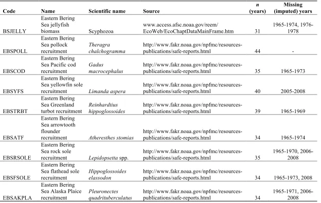
Table 1.S1 Descriptions and sources for biology time series included in study. ... 33

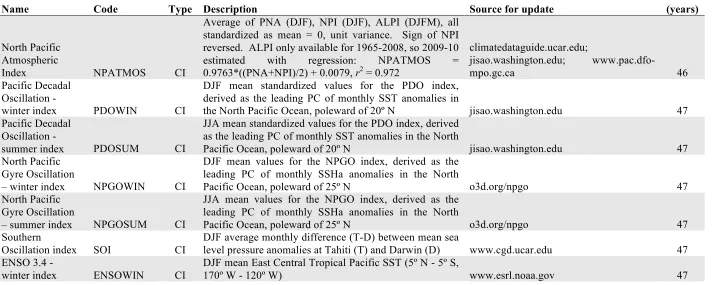
Table 1.S2 Climate data used in analysis: indices of leading modes of large-scale internal climate variability and regional climate parameters. ...37

Table 1.S3 Pairwise Pearson's correlation coefficients between indices of large-scale climate variability. ... 37

Table 1.S4 Pairwise Pearson's correlation coefficients for candidate variables used to explain regional biological variability. PDO, NPGO, AO, PNA, NPI and regional climate trend were smoothed with 3-year running mean. Climate trend was defined with residuals from regression of climate PC1 on the full set of internal climate modes. .37 Table 1.S5. Complete loadings for biology PC1 and PC2, sorted in decreasing order. ...38

Table 2.1 Summary of model selection results for Principle Component (PC) time series. .55 Table 2.S1. Description and sources for time series used in analysis. All time series values that span two calendar values are assigned to the year corresponding to January. Scientific names are given for the first occurrence of each taxon. ... 65

Table 2.S2. Loadings for PCA of large-scale climate index time series. ... 76

Table 2.S3. Loadings for PCA of local climate parameters. ...76

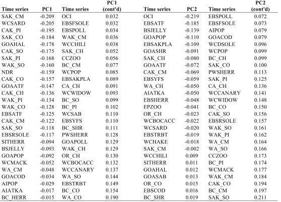
Table 2.S4 Loadings for PCA of biology time series. ... 77

Table 3.1 Loadings for PC1 of six regional climate parameters expected to respond strongly to the PDO and/or NPGO for periods before and after 1988/89 climate transition. Results come from separate PCA conducted on each period. Note changing patterns of correlation among loadings between periods. "Downwelling" refers to the persistently negative values of upwelling indices used in analysis. ... 89

Table 3.S1 Biology time series included in study. ...96

Table S3.2 Loadings for biology PC1 and PC2, sorted in decreasing order. ... 99

Table 4.1 Details of Alaskan crustacean fishery catch time series used in analysis...106

Table 5.1 Climate and biology time series used in analysis. ...128

Table 5.2 Correlations (Pearson's r) between SST PCs in this study and leading global SST modes. ... 135

Table 5.3. Complete loadings for first two axes of biological variability (PC1biol, PC2biol), in ascending order. For code explanations, see Table 5.1. ...141

Acknowledgements

Abstract

Rationale—Continental shelf ecosystems occasionally undergo "regime shifts"

– abrupt reorganization events that can have deleterious social and economic effects

on fishing communities that rely on affected species. Regime shifts are often

interpreted as transitions to alternative ecosystem states after external perturbations

such as fishing pressure cross a critical threshold; they have also been related to shifts

in modes of internal climate variability, such as the Pacific Decadal Oscillation and

North Atlantic Oscillation. However, hypotheses explaining regime shifts are

extremely difficult to test, given the multivariate nature of both stressors and

community response, the frequent paucity of data at adequate spatial and temporal

scales, possible non-linear and non-stationary relationships, and the use of

observational data that preclude strong inference. Furthermore, regime shifts have

often been invoked to explain ecological change without the consideration of

competing models, such as the accumulation of more gradual change over time. As a

result, both the nature of community-level biological change in continental shelf

systems (regime shifts vs. more gradual change), and the identity of factors producing

observed change, remain poorly resolved. Given increasing anthropogenic

disturbance to continental shelf ecosystems globally, there is a need both for better

understanding of the dynamics underlying sudden ecological change, and for tools

providing early detection of ecosystem change to allow for proactive management

measures that might minimize associated socio-economic disruption. Finally, the

regime shift concept is largely based on work in North Atlantic and North Pacific

ecosystems, and there is a need for studies in other areas to determine if the regime

shift model is widely applicable.

commercially-important fish and invertebrate populations), from the 1960s to the

present, covering the continental shelf between 30°N and 65°N. This dataset allowed

me to evaluate internal climate variability, commercial fishing and incremental

climate change as factors explaining decadal-scale biological variability (Chapter 1);

test competing models of gradual change and regime shifts for explaining

decadal-scale ecological variability (Chapter 2); develop an approach for evaluating possible

ecosystem shifts at the ends of time series (Chapter 2); test for non-stationary

biological responses to climate perturbations (Chapter 3); and test statistical tools for

early detection of ecosystem transitions (Chapter 4). In Chapter 5 I use the

methodology developed in the previous chapters to evaluate a data-poor situation in

southeast Australian continental shelf ecosystems, using nine climatic and 12

biological time series (seabird reproductive parameters and recruitment estimates for

commercially-important fish stocks) for the period 1967-present. This chapter tested

competing hypotheses invoking secular change and regime shifts to explain regional

climate-biology covariation.

Results—Analysis of northeast Pacific data showed that: the ecological change

that is frequently related to regime shifts in the literature is in many instances better

described as the result of incremental change over time (Chapters 1 and 2); commonly

held assumptions concerning the dominant role of internal climate variability as an

external driver on the system are poorly supported by data (Chapters 1 and 2);

assessment of incipient ecosystem shifts may be supported both by model-derived

statistical indicators and by formal evaluations of the length of observation needed to

evaluate ecosystem state (Chapters 2 and 4); and assumptions of stationarity are

inadequate for understanding community responses to climate variability (Chapter 3).

In southeast Australia (Chapter 5), I found that secular change best described

decadal-scale climatic and biological variability, with little evidence for a role of regime

shift-type variability in the system.

Introduction

Biological populations and communities are complex systems that may undergo

sudden transitions between alternative stable states. The importance of alternative

states in ecology, and the thresholds and discontinuities separating them, was

established during the 1960s and 1970s (Lewontin 1968, Holling 1973, May 1977),

though, as is the case with many concepts in ecology, precedents may be found

further back in the literature (e.g., Lotka 1956). Alternative stable states are

characterized by: 1) dramatic differences in state characteristics (e.g., density or

reproductive success for populations, species composition and trophic structure for

communities, human services for ecosystems); 2) different sets of internal and

external factors regulating the system; and 3) hysteresis, or critical perturbation

thresholds for transitions between states that depend on the direction of change in the

perturbation parameter (Scheffer et al. 2001, Beisner et al. 2003). Understanding and

predicting switches between alternative states have become leading research topics in

ecology (Scheffer and Carpenter 2003, Scheffer et al. 2012).

underscoring the importance of these transitions as a problem in applied marine

ecology applications, such as fisheries management.

Though alternative stable state theory has a long history in ecology, the

phenomenon remains best-studied in models (van Nes and Scheffer 2004, van Nes

and Scheffer 2007) and in simple ecosystems, notably shallow freshwater lakes

(Scheffer and van Nes 2007). Sudden transitions in continental shelf ecosystems have

long been offered as a possible example of alternative stable states in large, complex

ecosystems (Scheffer et al. 2001, Scheffer and Carpenter 2003), and there has been

interest by oceanographers and marine ecologists in applying alternative stable state

theory to understanding sudden transitions in marine systems (Choi et al. 2004, Collie

et al. 2004, Mantua 2004). However, progress along these lines remains slow.

Problems include the paucity of data at suitable spatial and temporal scales, the use of

observational data sets that are open to alternative interpretations (e.g., Frank et al.

2013, Greene 2013), the time (years to decades) needed to distinguish persistent states

from transitory reactions to perturbation (Frank et al. 2011), and the complexity of

multivariate processes in marine systems with unknown variables and relationships

(Overland et al. 2008). As a result of these difficulties, the question of whether

alternate stable state theory is applicable to abrupt reorganization events in continental

shelf ecosystems remains unanswered (Möllmann and Diekmann 2012), just as it

remains unanswered in much more tractable intertidal and nearshore demersal

ecosystems (Connell and Sousa 1983, Petraitis and Dudgeon 2004, Dudgeon et al.

2010).

As an alternative to stable state theory, another point of view holds that abrupt

reorganizations of continental shelf ecosystems are driven by sudden changes in

leading modes of internal climate variability (Mantua et al. 1997, Minobe 1997,

Hollowed et al. 2001, Greene et al. 2008, Greene et al. 2013). Since red noise

variability may produce decadal-scale periods when climate parameters depart from

their long-term mean (Rudnick and Davis 2003, Overland et al. 2006), a linear

ecological response to internal climate variability, perhaps dampened by the

generation time averaged across the community, might provide a more parsimonious

explanation for sudden ecosystem shifts than alternate stable state theory (Hsieh and

Ohman 2006, Di Lorenzo and Ohman 2013). However, abrupt community shifts may

also result from Gaussian climate variability coupled with non-linear biological

dynamics that are consistent with alternative stable states (Hsieh et al. 2005, Deyle et

al. 2013). The underlying dynamics remain uncertain.

There is widespread expectation that increased anthropogenic disturbance,

most notably through climate change, fishing, eutrophication and habitat destruction,

is making sudden ecosystem transitions more frequent (Folke et al. 2004). A stronger

theoretical underpinning would provide an important step towards understanding

these events, and theory has recently been developed to provide generic early warning

tools for sudden ecosystem transitions (Scheffer et al. 2009, Kéfi et al. 2013).

However, these approaches have so far been tested in models (Carpenter and Brock

2006, Guttal and Jayaprakash 2008), laboratory microcosms (Drake and Griffen 2010)

and small ecosystems amenable to experimental manipulation (Carpenter et al. 2011);

their utility in large, open ecosystems, such as those on continental shelves, remains

largely untested (Scheffer et al. 2012).

In the order in which they are presented, the specific questions addressed by

the thesis are:

Chapter 1) What are the set of external perturbations driving abrupt shifts? As

is the case with most questions in ecology, the answer is likely to be contingent on

system- and time-dependent factors (Lawton 1999). However, northeast Pacific

ecosystems (i.e., the California Current, Gulf of Alaska and eastern Bering Sea large

marine ecosystems [LMEs]) provide an excellent case study for answering this

question. While internal climate variability has long been associated with

decadal-scale variability in these ecosystems (Trenberth and Hurrell 1994, Mantua et al. 1997,

Minobe 1997), the seminal studies documenting the ecological importance of internal

climate variability often made no attempt to test statistical hypotheses explaining

observed ecosystem changes (Hollowed and Wooster 1992, Mantua et al. 1997,

Anderson and Piatt 1999). This was understandable given the statistical techniques

and computing power that were generally available in the 1990s (Daskalov et al.

2003), but even with advances in those fields, studies continue to invoke internal

climate variability as a leading driver of decadal-scale, community-level biological

change, without examining competing hypotheses invoking factors such as secular

change in climate or commercial fishing (e.g., Francis and Hare 1994, Mantua et al.

1997, Anderson and Piatt 1999, Hare and Mantua 2000, Beamish et al. 2004, Litzow

2006, Kaeriyama et al. 2009). This chapter uses updates to previously-published

biological time series from two northeast Pacific LMEs (Gulf of Alaska and eastern

Bering Sea) to examine the importance of internal climate variability, secular climate

change and commercial fishing as drivers of community-level biological change from

1965-present. Overfishing and extensive habitat loss for anadromous fishes in the

California Current LME (Nehlsen 1997, Harvey et al. 2006) were judged too difficult

to account for in statistical models, so data from that ecosystem were excluded from

this chapter.

(Spencer et al. 2012). Although a number of incremental forcing mechanisms are at

work in the northeast Pacific (e.g., secular climate change, persistant fishing

removals, habitat loss; Nehlsen 1997, Gillett et al. 2003, Harvey et al. 2006, Schwing

et al. 2010), making the presence of persistent, incremental ecological change a

reasonable expectation, comparisons of gradual and abrupt models for ecological

change across the region have not been previously published. Additionally, after the

dramatic region-wide ecological transition that accompanied the 1976/77 shift in the

PDO (Anderson and Piatt 1999, Hare and Mantua 2000, Benson and Trites 2002),

there has been a history of attempts to provide early recognition of subsequent shifts

in this region (e.g.; Bond et al. 2003, Peterson and Schwing 2003, Hatch 2013).

However, in spite of the advancement of statistical techniques to test for shifts at the

ends of time series (e.g., Rodionov 2006), many years of data after a putative shift are

required to distinguish interannual noise from low-frequency variability (Litzow

2006). This chapter presents a formal approach for assessing the length of

observation needed for evaluating potential shifts.

Chapter 3) Do continental shelf communities show non-stationary responses to

perturbations such as climate change and fishing? Non-stationary relationships with

external variables are a hallmark of alternate stable state theory (Scheffer et al. 2001,

Beisner et al. 2003). Recent work in the northeast Pacific has produced a number of

examples of populations that are controlled by different sets of external and internal

factors at different points in time, producing correlations with individual driver

parameters that arise and disappear (Ciannelli et al. 2004, Ciannelli et al. 2005,

Litzow and Ciannelli 2007, Bacheler et al. 2012, Ciannelli et al. 2012, Sugihara et al.

2012, Deyle et al. 2013). However, little (or no) research has been published on

non-stationary relationships between regional community variability and external drivers.

By applying a model-selection approach (Burnham and Anderson 2002) using

threshold generalized additive models that fit non-parametric and non-stationary

driver-response relationships, I test for non-stationary community responses to

perturbations of northeast Pacific ecosystems.

generic indicators suggest an avenue for deriving useful fisheries management tools

from ecological theory, the idea is in its infancy, with empirical tests to date mostly

limited to laboratory microcosms and simple, easily manipulated ecosystems, with

few tests in the large, open ecosystems that are the purview of fisheries management

(Scheffer et al. 2012). This chapter uses a set of historical catch data from 14

crustacean fisheries in Alaska, running from the 1960s to the 2000s, to test for the

presence of proposed indicator behaviors (increasing spatial variance and skewness in

catch) prior to stock collapse.

Chapter 1 Reassessing regime shifts in the North Pacific:

incremental climate change and commercial fishing are necessary

for explaining decadal-scale biological variability

Abstract

Introduction

Red noise in leading modes of internal climate variability may produce "square wave"

behavior consisting of abrupt switches between steady states (Minobe 1999, Rudnick and

Davis 2003, Di Lorenzo and Ohman 2013). Recognition of abrupt shifts in leading modes of

basin-scale climate variability (hereafter "climate regime shifts") was a major advance in

marine ecology, as these events explain biological variability that is coherent at very large

spatial scales, such as inverse patterns of salmon (Oncorhynchus spp.) production in the

northern and southern Northeast Pacific and inverse patterns of sardine (Engraulis spp.) and

anchovy (Sardinops

spp.) production in a variety of temperate ecosystems (Mantua et al.

1997, Francis et al. 1998, Chavez et al. 2003). Climate regime shifts are expected to continue

under anthropogenic climate change (Overland and Wang 2007), and understanding the

impacts of these shifts relative to anthropogenic climate change and other anthropogenic

impacts, such as fishing, is vital for understanding and managing marine ecosystems.

Möllmann and Diekmann 2012). In contrast, while some areas of the North Pacific have

been overfished (Harvey et al. 2006, Worm et al. 2009, Milazzo 2012), other areas, such as

the eastern Bering Sea and northern Gulf of Alaska, have largely been free from overfishing

(Litzow and Urban 2009, Milazzo 2012), and have been proposed as models of generally

successful fisheries management (Witherell et al. 2000, Stram and Evans 2009, Worm et al.

2009). These areas are also strongly affected by leading global modes of internal climate

variability (i.e., the El Niño-Southern Oscillation [ENSO], Pacific Decadal Oscillation [PDO]

and North Pacific Gyre Oscillation [NPGO] patterns; Messié and Chavez 2011).

Accordingly, a view of internal climate variability as the most important driver of

community-level variability, especially across climate regime shifts in 1976/77 and 1988/89,

has developed in this region, and studies of the ecological effects of internal climate

variability have often failed to consider alternate hypotheses invoking fishing or other human

activities, or climate trends independent of internal climate variability (e.g., Francis and Hare

1994, Mantua et al. 1997, Anderson and Piatt 1999, Hare and Mantua 2000, Beamish et al.

2004, Litzow 2006, Di Lorenzo et al. 2008, Kaeriyama et al. 2009, Möllmann and Diekmann

2012). Although studies focusing solely on internal climate variability were necessary for

developing understanding of the ecological effects of climate regime shifts, studies that

simultaneously consider alternate hypotheses are a necessary further step for understanding

the relative importance of different external drivers in producing community-level variability

(Choi et al. 2005). Understanding the potential impacts of low-frequency climate variability

relative to other external forcing mechanisms is particularly important given the ongoing

potential for disruptive climate regime shifts in the North Pacific (Zwolinski and Demer

2012, Hatch 2013, Litzow and Mueter 2014).

(Alaskan waters in the U.S. Exclusive Economic Zone) where habitat loss has been much less

pervasive (Nehlsen 1997). The specific goals of our study were 1) to assess the ability of a

comprehensive set of leading modes of internal climate variability to explain decadal-scale

patterns of climatic variability within our study region; 2) to assess the ability of the same

modes of internal climate variability to explain decadal-scale biological variability in the

region; and 3) to compare the evidence for the internal climate modes, climate change

independent of those modes, and commercial fishing (total biomass removals) as explanatory

variables

for

observed

biological

variability.

Although coherent basin-scale

biological variability has been

studied in the North Pacific for

~20 years (e.g., Francis and

Hare 1994), this is, to our

knowledge, the first study that

has used statistical models to

evaluate the relative evidence

for these different drivers as

the causative agents.

Materials and Methods

Data

complete time series descriptions and sources are in Table 1.S1. Justification for the

inclusion of various time series, especially salmon catch data, is given by Hare et al. (1999)

and Hare and Mantua (2000).

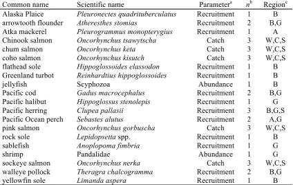
Table 1.1 Summary of the 36 biological time series used in analysis, ordered by common name. Complete details in Table 1.S1.

a _{Recruitment = estimated recruitment, log-transformed and lagged to cohort year; Catch =} commercial catch, log-transformed and lagged to year of ocean entry; Abundance = survey-estimated biomass

b _{number of time series}

c _{A = Aleutian Islands (part of Bering Sea ecosystem); B = Bering Sea; C = central Alaska (i.e.,} western Gulf of Alaska); G = Gulf of Alaska; W = western Alaska (Bering Sea with minor contribution from the Arctic); S = Southeast Alaska (part of Gulf of Alaska ecosystem).

Common name Scientific name Parametera _nb _Regionc

Alaska Plaice Pleuronectes quadrituberculatus Recruitment 1 B arrowtooth flounder Atheresthes stomias Recruitment 2 B,G Atka mackerel Pleurogrammus monopterygius Recruitment 1 A Chinook salmon Oncorhynchus tsawytscha Catch 3 W,C,S

chum salmon Oncorhynchus keta Catch 3 W,C,S

coho salmon Oncorhynchus kisutch Catch 3 W,C,S

flathead sole Hippoglossoides elassodon Recruitment 1 B Greenland turbot Reinhardtius hippoglossoides Recruitment 1 B

jellyfish Scyphozoa Abundance 1 B

Pacific cod Gadus macrocephalus Recruitment 2 B,G

Pacific halibut Hippoglossus stenolepis Recruitment 1 G Pacific herring Clupea pallasii Recruitment 3 B,G,S Pacific Ocean perch Sebastes alutus Recruitment 2 A,G

pink salmon Oncorhynchus gorbuscha Catch 3 W,C,S

rock sole Lepidopsetta spp. Recruitment 1 B

sablefish Anoplopoma fimbria Recruitment 1 G

shrimp Pandalidae Abundance 1 G

sockeye salmon Oncorhynchus nerka Catch 3 W,C,S

walleye pollock Theragra chalcogramma Recruitment 2 B,G

yellowfin sole Limanda aspera Recruitment 1 B

as the Northern Annular Mode] and Pacific-North American Pattern [PNA]), and the North

Pacific Index (NPI), the average of regional SLP that captures variability in the Aleutian

Low. This set includes the most important climate indices implicated by studies of climate

regime shifts in the North Pacific (Minobe 1999, Overland et al. 1999, Mantua and Hare

2002, Schwing et al. 2003, Overland and Wang 2005, Di Lorenzo et al. 2008, Messié and

Chavez 2011). As a measure of El Niño-Southern Oscillation (ENSO) activity we included

annual mean values of the Multivariate ENSO Index (MEI), lagged one year to account for

delay in propagation of the tropical ENSO signal to our study region (sources for climate

indices in Table 1.S2). Leading modes for Northern Hemisphere SLP and detrended North

Pacific SST show the most coherent variability in the winter season, due to a decadal-scale

intensification in winter atmospheric circulation over the North Pacific, and a seasonal peak

in midlatitude response to tropical SST forcing during the winter (Yeh et al. 2011). We

therefore used winter values for the internal climate modes in our analysis, with the months

used conforming to convention for

each index (NDJFM for the PDO and

NPGO, JFM for the AO and PNA,

DJF for the NPI).

total biomass removals (retained catch and, where available, discards) for domestic (U.S.)

and international fleets (Litzow and Urban 2009).

Analysis

Our analysis sought to derive the best explanations for observed patterns of decadal-scale

climatic and biological variability in our study region, using a suite of potential covariates

(drivers). A multi-step analytical approach was required to summarize multivariate

variability in the response variables and to account for temporal autocorrelation in both

drivers and response variables, and for multicollinearity in drivers. We summarize our

analysis around the three study goals, and provide a schematic diagram outlining our

analytical steps in Fig. 1.2.

We began analysis by using principal components analysis (PCA) to summarize

variability in response variables (regional climate and biology). We were interested in the

most important axes of ecological variability, so analysis was restricted to PC1 for the

regional climate variables, and PC1 and 2 for biology variables. The "broken-stick" and

bootstrapped-

λ

approaches of Jackson (1993) were used to confirm that these PCs were

absolute value for the corresponding PC score across all years of the time series, we judged

that too much uncertainty had been introduced by estimating missing values, and these

estimates were excluded from further analysis.

Goal 1: Assess the ability of large-scale climate modes to explain regional climatic

variability

We tested for the ability of the large-scale climate modes to explain observed patterns of

regional climate variability using multiple linear regression (Fig. 1.2). The use of linear

models is consistent with the linear methods (EOFs/PCA) used to derive the modes from

anomaly fields of fundamental climate parameters. This analysis was conducted both with

the full model (i.e., invoking the PDO, NPGO, AO, PNA, NPI and MEI) in order to

maximize the proportion of variance explained, as well as with the best model, as determined

by Akaike's Information Criterion adjusted for small sample size (AICc). Residuals from

regression models were tested for significant trends, which would indicate both that the

model violated the assumption of independent residuals, and that the model failed to explain

a coherent pattern of regional climate variability. To calculate appropriate

P–values for

residual trends in the presence of potential serial autocorrelation, we employed a generalized

least-squares (GLS) approach with first-order autocorrelated residuals and year as a linear

predictor variable, using the package "nlme" in R (Pinheiro and Bates 2000).

Multicollinearity was present among the large-scale climate modes (Table 1.S3), so we did

not calculate P-values for individual covariates (Graham 2003).

Goal 2) Assess the ability of the large-scale climate modes to explain regional biological

variability

biological systems to respond strongly to changes in mean climate state, but to be more

resilient to stochastic (interannual) variability around that mean. Second, we expected the

early life-history processes that dominate the time series in our study (i.e., recruitment and

juvenile survival) to be most sensitive to processes occurring at lags of -1 (e.g., adult feeding,

migration and spawning behavior), 0 (e.g., advection of eggs and larvae) and 1 (e.g., juvenile

survival) years. The inclusion of climate data at lag 1 year through smoothing is justified by

the fact that most of the biological time series in our study had also been lagged between 1

and 8 years in order to reflect year class strength (for groundfish and herring) or cohort

strength at ocean entry (for salmon).

We report results for the five best models that could be constructed for each biology

PC when invoking only the large-scale climate modes as explanatory variables. We

recognize that selection from the full set of models is not typically recommended (Burnham

and Anderson 2002), but in this case there is strong support for a role of each individual

parameter in structuring ecological variability (e.g., Minobe 1999, Overland et al. 1999,

Mantua and Hare 2002, Overland and Wang 2005, Di Lorenzo et al. 2008, Schwing et al.

2010), so our goal was to evaluate the ability of the best models invoking these modes to

explain biological variability; hence model selection from a global set of covariates was

judged to be appropriate in this instance. Model selection was conducted by minimizing the

generalized cross validation (GCV) score, which rewards model parsimony and predictive

power. We then tested the best five models for each biology PC score for significant linear

trends in residuals, again using a GLS approach.

trends with GLS, and compare support for these models (in terms of GCV scores) with the

five best models for each PC score that could be constructed only from the climate modes.

Evaluating the support for individual covariates as drivers of biological variability could

not rely on

P-values, as multicollinearity was also present in the set of external variables for

this analysis (Table 1.S4). We

therefore

evaluated

the

importance

of

individual

parameters from the best model

for each PC in terms of effect

size and evidence for being

included in the true model.

Effect size was calculated as

the proportion of deviance

uniquely explained by each

explanatory variable. For each

biology PC, we fit a set of

reduced models derived from

the best GAM, removing each forcing variable in turn while maintaining the smoothing

parameters for the remaining variables equal to the smoothing parameters from the full

model. If

F = the full model,

N = the null model (i.e.,

, with 0% of deviance

explained), and

X = the reduced model, with variable

x removed, then the proportion of

deviance uniquely explained by

x can be calculated as: (deviance(X) – deviance(F)) /

deviance(N) (S. Wood, public comm., accessed 2 July 2011, R Project / R Help,

r.789695.n4.nabble.com/variance-explained-by-each-term-in-a-GAM-td836513.html). We

also evaluated the evidence supporting individual parameters by summing Akaike weights

(w) over the set of models including a given parameter (Burnham and Anderson 2002).

Results

Goal 1

(0.53), with a weaker loading on Bering Sea ice cover (-0.17). Climate PC1 showed a

significant linear trend during 1965-2008 (GLS, P = 0.02), indicating increasing winter SST,

increasing freshwater input, and decreasing winter SLP during that time. This trend could

not be completely explained by the modes of

internal climate variability; residuals from the

linear model invoking the full set of climate

modes (PDO, NPGO, AO, PNA, NPI, MEI)

also showed a significant linear trend (GLS, P

= 0.03, Fig. 1.3). This trend indicated that the

model failed to meet assumptions of

independent residuals. The best linear model

that could be constructed from the climate

modes alone (invoking the PDO and NPI)

showed a similar trend in residuals (GLS, P =

0.03). Since the residual trend from the full

model captures a pattern of coherent climate

variability that is by definition independent of

the climate modes, we used the residuals from

the full model, smoothed with a 3-year

running mean, as an additional candidate

covariate in models of variability in biology

PC series. We refer to this additional

covariate as the "climate trend"; time series of

all candidate covariates for models of

biological variability are plotted in Fig. 1.S1.

Goal 2

Biology PC1 explained 30.6% of total variance, and showed strong loadings (absolute value

≥ 0.2) on fourteen time series. Eleven salmon time series, from across the study area, showed

negative loadings, as did Gulf of Alaska halibut and Bering Sea rock sole; Gulf of Alaska

shrimp showed a positive loading (Fig. 1.4a). Biology PC2 explained 12.4% of total

variance, and showed strong loadings on ten time series: negative loadings by Bering Sea

jellyfish and arrowtooth flounder and Gulf of Alaska Pacific Ocean perch and arrowtooth

flounder; and positive loadings by all five species of Bering Sea salmon and Prince William

Sound herring (Fig. 1.4b; complete PCA loadings in Table 1.S5).

Our biology PC1 and 2 were well correlated, for the period of overlap, with PC1 and 2 from

the biology time series for the entire northeast Pacific originally published by Hare and

Mantua (2000; PC1: r = 0.96, PC2: r = 0.62). The time series of biology PC1 scores captures

the well-documented transition (Anderson and Piatt 1999, Hare and Mantua 2000), during the

1970s and 1980s, from a crustacean-abundant state to a groundfish- and salmon-abundant

state (Fig. 1.5a). Estimates for biology PC2 scores in 1965-1973 had SD values > the mean

absolute value of PC2 scores across the time series, so these years were excluded from

analysis of factors forcing PC2 variability. The remainder of the time series was associated

with a transition, in the 1990s, from abundant Bering Sea salmon (all five spp.) and Prince

William Sound herring to abundant jellyfish and arrowtooth flounder in the Bering Sea, and

Pacific Ocean perch and arrowtooth flounder in the Gulf of Alaska (Fig. 1.5c).

The best statistical models of biological variability that could be constructed from the

climate modes alone invoked the AO and PDO for biology PC1, and the AO for biology PC2.

However, both of these models showed significant linear trends in residuals (GLS; P ≤ 0.01;

Fig. 1.5b,d), indicating that they failed to capture directional trends in the leading modes of

biological variability, thereby violating the assumption of independent residuals. Similar

significant trends in residuals were shown for all five of the best models that could be

constructed for each PC series from the climate modes alone (Table 1.2).

Goal 3

When the full set of candidate forcing mechanisms (internal climate modes, the climate trend

and commercial catch) was employed, four of the five best models for biology PC1, and all

five of the best models for biology PC2, met the assumption of independent residuals (GLS,

P

≥ 0.09, Table 1.2). The best model for biology PC1 using the full set of candidate

variables invoked commercial catch, the climate trend, the MEI, the NPI and the PDO, with

the climate trend accounting for the highest proportion of unique deviance (Fig. 1.6a-e).

Evidence across models also showed the climate trend to be the most likely of these five

covariates to be included in the true model (Fig. 1.6f). The best model for biology PC2 that

could be constructed from the full set of candidate parameters invoked the AO, commercial

catch, the climate trend, the NPGO and the PNA as explanatory variables, with commercial

catch explaining 1.8 times the unique deviance of the covariate with the next-greatest effect

size (Fig. 1.6g-k). Akaike weights showed strongest support for commercial catch and the

NPGO as explanatory variables for biology PC2 (w > 0.99, Fig. 1.6l).

Discussion

1999). Advances in statistics and computing over the last decade have made this problem

more tractable, and the non-parametric regression (i.e., GAM) approach that we use here is

now commonly employed to make inferences about the factors producing non-linear behavior

in biological time series (Daskalov et al. 2003, Ciannelli et al. 2004, Litzow and Ciannelli

2007, Brodeur et al. 2008, Stige et al. 2010, Mueter et al. 2011, Siddon et al. 2011, Smart et

al. 2012). We show conclusively that leading modes of internal climate variability in the

North Pacific are by themselves inadequate to explain leading axes of climatic (Fig. 1.3) and

biological (Fig. 1.5, Table 1.2) variability in the Gulf of Alaska and Bering Sea ecosystems

over a 44-year period, as indicated by significant trends in model residuals. However, when

the set of candidate covariates was enlarged to include the residual trend in climate PC1 and a

time series of total commercial fishery biomass removals, best GAMs for biology PC1 and

PC2 met assumptions of independent residuals and provided high degrees of explanatory

power (Fig. 1.6, Table 1.2). These results suggest that the view of decadal-scale ecological

variability in this study region as being dominated by internal climate variability (e.g., Hare

and Mantua 2000, Benson and Trites 2002, Möllmann and Diekmann 2012) should be

expanded to include the effects, at least, of commercial fishing and climate change unrelated

to internal variability. Additionally, linear effects of the climate trend (Fig. 1.6b) and

commercial catch (Fig. 1.6h) on biology PC1 and PC2, respectively, also suggest the

importance of incremental ecosystem forcing on biological change in the region, which

argues against an understanding of regional ecosystem dynamics based entirely on abrupt

shifts between quasi-steady states (Lees et al. 2006, Spencer et al. 2012, Litzow and Mueter

2014).

herring populations respond to variability in ice cover and SST (Tojo et al. 2007, Deriso et al.

2008); jellyfish populations respond to variability in SST, ice cover, advection and wind

mixing (Brodeur et al. 2008); and shrimp populations respond to variability in SST and

bottom temperature (Litzow and Ciannelli 2007, Mueter and Litzow 2008). The coherent

large-scale patterns of climate variability that are summarized by the climate modes in our

study affect individual populations through simultaneous change to the set of climate

parameters that are important for regulating particular populations in particular locations

(Mantua and Hare 2002, Di Lorenzo et al. 2008). Simultaneous regional change in SST, SLP

and freshwater discharge that is independent of those climate modes (Fig. 1.3), could

plausibly be expected to regulate the populations loading heavily on biology PC1 in a similar

fashion. Coherent community-level variability in turn arises both from covariation among

populations exposed to large-scale patterns of climate variability (Wilderbuer et al. 2002,

Mueter et al. 2007) and from climate regulation of species interactions, such as predation and

competition (Litzow and Ciannelli 2007, Poloczanska et al. 2008). However, emergent

properties, feedbacks, synergistic effects and other behaviors of complex systems preclude a

simple understanding of the factors regulating community-level variability from the sum of

population-level responses (Drake 1991, Scheffer et al. 2001). Additionally, observational

studies are unable to distinguish the factors maintaining a community in its current state from

the factors that initially produced the observed state (Drake 1991), or to distinguish, a priori,

persistent community states from transients (Frank et al. 2011). These considerations make a

mechanistic understanding of the apparent relationship between the residual climate trend and

biology PC1 (Fig. 1.6b,f) beyond the scale of this study. Additionally, our results support the

view that internal climate variability is an important, though not sufficient, explanation for

community variability summarized by biology PC1. The NPI and PDO indices track the

atmospheric and oceanic imprints, respectively, of a single pattern of large-scale climate

variability (Minobe 1999, Mantua and Hare 2002, Schwing et al. 2003), which is

mechanistically related to ENSO variability (Newman et al. 2003). The combined effect size

of these indices (Fig. 1.6c-e) supports the view that low-frequency internal climate variability

remains critical for understanding large-scale ecological variability in the North Pacific,

especially with recent interest in indications of a possible switch to persistently

PDO-negative conditions in the mid-late 2000s (Cai and van Rensch 2012, Zwolinski and Demer

2012, Hatch 2013, Litzow and Mueter 2014).

surveys (Worm et al. 2009), the number of stocks under rebuilding plans relative to other

ecosystems under U.S. jurisdiction (Milazzo 2012), and stability in catches at decadal time

scales (Litzow and Urban 2009). Our finding that commercial catch plays a leading role in

regulating biology PC2 (Fig. 1.6h,l) therefore occurs in the absence of ongoing overfishing.

Inference of a relationship between commercial catch and biology PC2 variability is

supported by the exploitation history of taxa loading heavily on this axis of variability; the

four populations showing loadings

≤ -0.2, associated with an increasing trend, are either not

subject to a directed fishery (Bering Sea jellyfish, Bering Sea and Gulf of Alaska arrowtooth

flounder) or have been recovering from overfishing during the 1960s (Gulf of Alaska Pacific

Ocean perch, Litzow and Urban 2009). Commercial fishing has the potential to change

community composition (Harvey et al. 2006) and the linear relationship between total catch

and biology PC2 scores (Fig. 1.6h) is consistent with a direct, ongoing influence of fishing

pressure on community structure. In particular, awareness has been growing for several years

that increases in arrowtooth flounder populations in the Gulf of Alaska and Bering Sea may

reflect the lower exploitation pressure on this species relative to other groundfish, with a

positive feedback created by increased arrowtooth flounder predation on other groundfishes

(Bailey 2000, Zador et al. 2011, Bailey et al. 2012).

accumulation of anthropogenic greenhouse gasses (Gedalof et al. 2002), variability in these

modes is to some degree now affected by anthropogenic forcing (Morgenstern et al. 2010,

Bonfils and Santer 2011). Therefore, just as the residual climate trend in our study cannot be

formally attributed to anthropogenic forcing, the climate modes cannot be treated as tracking

purely natural climate variability. The distinction between ecological effects of natural and

anthropogenic climate change cannot therefore be made from our analysis, and we simply

interpret our results as demonstrating the regional ecological importance of observed climate

change that is independent of the leading climate modes. In summary, modes of internal

climate variability remain important for understanding decadal-scale, basin-scale marine

ecosystem variability, but a view of these modes as the most important factor in driving

large-scale patterns of ecological variability may be obsolete, even in areas that are subject to

strong internal climate variability and free of overfishing.

Acknowledgements