Hunting for Tractable Languages for Judgment Aggregation
Ronald de Haan
Institute for Logic, Language and Computation University of Amsterdam
Abstract
Judgment aggregation is a general framework for collective decision making that can be used to model many different set-tings. Due to its general nature, the worst case complexity of essentially all relevant problems in this framework is very high. However, these intractability results are mainly due to the fact that the language to represent the aggregation domain is overly expressive. We initiate an investigation of representation lan-guages for judgment aggregation that strike a balance between (1) being limited enough to yield computational tractability results and (2) being expressive enough to model relevant ap-plications. In particular, we consider the languages of Krom formulas, (definite) Horn formulas, and Boolean circuits in decomposable negation normal form (DNNF). We illustrate the use of the positive complexity results that we obtain for these languages with a concrete application: voting on how to spend a budget (i.e., participatory budgeting).
Introduction
Judgment aggregation is a general framework to study methods for collective opinion forming, that has been in-vestigated in the area of computational social choice (see, e.g., Endriss 2016, Grossi and Pigozzi 2014). The framework is set up in such a general way that it can be used to model an extremely wide range of scenarios—including, e.g., the setting of voting (Dietrich and List 2007). On the one hand, this generality is an advantage: methods studied in judgment aggregation can be employed in all these scenarios. On the other hand, however, this generality severely hinders the use of judgment aggregation methods in applications. Because there are no restrictions on the type of aggregation settings that are modeled, relevant computational tasks across the board are computationally intractable in the worst case. In other words, no performance guarantees are available that warrant the efficient use of judgment aggregation methods for applications—not even for simple settings. For example, com-puting the outcome of a judgment aggregation scenario is NP-hard for all aggregation procedures studied in the literature that satisfy the rudimentary quality condition ofconsistency
(Endriss and De Haan 2015; De Haan and Slavkovik 2017; Lang and Slavkovik 2014).
Copyright c2018, Association for the Advancement of Artificial Intelligence (www.aaai.org). All rights reserved.
These negative computational complexity results are in many cases due purely to the expressivity of the language used to represent aggregation scenarios (full propositional logic, or CNF formulas)—not to the structure of the sce-nario being modeled. In other words, the known negative complexity results draw an overly negative picture
To correct this gloomy and misleading image, a more de-tailed and more fine-grained perspective is needed on the way that application settings are modeled in the general frame-work of judgment aggregation. In this paper, we take a first look at the complexity of judgment aggregation scenarios using this more sensitive point of view. That is, we initiate an investigation of representation languages for judgment aggre-gation that (1) are modest enough to yield positive complexity results for relevant computational tasks, yet (2) are general enough to model interesting and relevant applications.
Concretely, we look at several restricted propositional languages that strike a balance between expressivity and tractability in other settings, and we study to what extent such a balance is attained in the setting of judgment aggre-gation. In particular, we look at Krom (2CNF), Horn and definite Horn formulas, and we consider the class of Boolean circuits in decomposable negation normal form (DNNF). We study the impact of these restricted languages on the com-plexity of computing outcomes for a number of judgment aggregation procedures studied in the literature. We obtain a wide range of (positive and negative) results. Most of the results we obtain are summarized in Tables 3, 4 and 5, located in later sections.
In particular, we obtain several interesting positive com-plexity results for the case where the domain is represented using a Boolean circuit in DNNF. Additionally, we illus-trate how this representation language of Boolean circuits in DNNF—that combines expressivity and tractability—can be used to get tractability results for a specific application: voting on how to spend a budget. This application setting can be seen as an instantiation of the setting ofParticipatory Budgeting(see, e.g., Benade et al. 2017).
of computing outcomes for judgment aggregation procedures has been studied by, a.o., Endriss, Grandi, and Porello (2012), Endriss et al. (2016), Endriss and De Haan (2015), De Haan and Slavkovik (2017) and Lang and Slavkovik (2014). See Table 2 for complexity results that are relevant for this paper.
Roadmap We begin by explaining the framework of judg-ment aggregation. We then study to what extent the known languages of Krom and (definite) Horn formulas lead to suit-able results for judgment aggregation. We continue with look-ing at the class of DNNF circuits—studied in the field of knowledge compilation—and we illustrate how results for this class of circuits can be used for a concrete application of judgment aggregation (that of voting on how to allocate a budget). We conclude with outlining some promising ways in which the research path that we set out can be followed.
An overview of notions from propositional logic and com-putational complexity theory that we use can be found in the appendix. The proofs of some results are omitted from the main paper and are located in the additional material at the end—these results are marked with a star (?).
Judgment Aggregation
We begin by introducing the setting of Judgment Aggregation (Dietrich 2007; Endriss 2016; Grossi and Pigozzi 2014; List and Pettit 2002). In this paper, we will use a variant of the framework that has been studied by, e.g., Grandi (2012), Grandi and Endriss (2013) and Endriss et al. (2016).1
LetI ={x1, . . . , xn}be a finite set ofissues, in the form
of propositional variables. Intuitively, these issues are the topics about which the individuals want to combine their judgments. A truth assignmentα : I → {0,1} is called aballot, and represents an opinion that individuals and the group can have. We will also denote ballotsαby a binary vec-tor(b1, . . . , bn)∈ {0,1}n, wherebi =α(xi)for eachi ∈ [n]—we use[n]to denote{1, . . . , n}for eachn∈N. More-over, we say that(p1, . . . , pn)∈ {0,1, ?}nis apartial
bal-lot, and that(p1, . . . , pn)agrees with a ballot(b1, . . . , bn)
ifpi = bi wheneverpi 6=?, for alli∈ [n]. We use an
in-tegrity constraintΓto restrict the set of feasible opinions (for both the individuals and the group). The integrity constraintΓ is a propositional formula (or more generally, a single-output Boolean circuit), whose variables can includex1, . . . , xn. We
define the setR(I,Γ)ofrational ballotsto be the ballots (forI) that are consistent with the integrity constraintΓ. We say that finite sequencesr ∈ R(I,Γ)+ of rational ballots
areprofiles. A profile contains a ballot for each individual participating in the judgment aggregation scenario. Where convenient we equate a profiler = (r1, . . . , rp)with the
multiset containingr1, . . . , rp.
Ajudgment aggregation procedure(orrule), for the setI
of issues and the integrity constraintΓ, is a functionF that takes as input a profiler∈ R(I,Γ)+, and that produces a non-empty set of ballots. A procedureFis calledconsistent
1
This framework is also known under the name ofbinary aggre-gation with integrity constraints, and can be used interchangeably with other Judgment Aggregation frameworks from the literature —as shown by Endriss et al. (2016).
if for allI,Γandrit holds that eachr∗∈F(r)is consistent withΓ. Consistency is a central requirement for judgment aggregation procedures, and all rules that we consider in this paper are consistent.
An example of a simple judgment aggregation procedure is themajority rule(defined for profiles with an odd number of ballots). We let the majority outcomemrbe the partial ballot
such that for eachx∈ I,mr(x) = 1if a strict majority of
ballotsri∈rsatisfyri(x) = 1,mr(x) = 0if a strict
major-ity of ballotsri ∈rsatisfyri(x) = 0, andmr(x) =?
oth-erwise. The majority rule returns the majority outcomemr.
The majority rule is efficient to compute, but is not consistent (as shown in Example 1).
Example 1. Consider the judgment aggregation scenario. whereI ={x1, x2, x3},Γ = (¬x1∨ ¬x2∨ ¬x3), and the
profiler= (r1, r2, r3)is as shown in Table 1. The majority
outcomeMAJ(r)is inconsistent withΓ.
r x1 x2 x3
r1 1 1 0
r2 1 0 1
r3 0 1 1
[image:2.612.384.496.260.332.2]MAJ(r) 1 1 1
Table 1: Example of a judgment aggregation scenario.
Judgment Aggregation Procedures
Next, we introduce the judgment aggregation rules that we use in this paper. These procedures are all consistent and are many of the ones that have been studied in the literature (for an overview see, e.g., Lang et al. 2017).
Several procedures that we consider can be seen as instan-tiations of a general template:scoring procedures. LetIbe a set of issues andΓbe an integrity constraint. Moreover, let s : R(I,Γ)×Lit(I) → Nbe ascoring functionthat assigns a value to each literal l ∈ Lit(I)with respect to a ballot r ∈ R(I,Γ). The scoring judgment aggregation procedureFsthat corresponds tosis defined as follows:
Fs(r) = arg max
r∈R(I,Γ)
X
ri∈r
X
l∈Lit(I)
r(l)=1
s(ri, l).
That is, Fs selects the rational ballots r ∈ R(I,Γ) that maximize the cumulative score for all literals agreeing withr
with respect to all ballotsri ∈r.
Themedian (or Kemeny) procedureMEDis based on the scoring function and is defined by lettingsK(r, l) = r(l) for eachr ∈ R(I,Γ) and eachl ∈ Lit(I). Alternatively, theMEDprocedure can be defined as the rule that selects the ballotsr∗∈ R(I,Γ)that minimize the cumulative Hamming distance to the profiler. TheHamming distancebetween two ballotsr, r0isdH(r, r0) =|{x∈ I :r(x)6=r0(x)}|.
The reversal scoring procedure REV is based on the scoring function sR(r, l) such that sR(r, l) = minr0∈R(I,Γ),r0(l)=0dH(r, r0) for each r ∈ R(I,Γ) and
the minimal number of issues whose truth value needs to be flipped to get a rational ballotr0that setslto false.
Themax-card Condorcet (or Slater) procedure MCC is also based on the Hamming distance. Let r be a pro-file. The MCC procedure is defined by letting MCC(r) = arg minr∗∈R(I,Γ)dH(r∗, mr). That is, theMCC procedure
selects the rational ballots that minimize the Hamming dis-tance to the majority outcomemr.
TheYoung procedure YOUNGselects those ballots that can be obtained as a rational majority outcome by delet-ing a minimal number of ballots from the profile. Letrbe a profile, and let ddenote the smallest number such that deletingdindividual ballots fromrresults in a profiler0
such thatmr0 is a complete and rational ballot. We let the
outcomeYOUNG(r)of the Young procedure be the set of ra-tional ballotsr∗such that deletingdindividual fromrresults in a profiler0withmr0 =r∗.
The Max-Hamming procedure MAXHAM is also based on the Hamming distance. Let r be a single ballot, and let r = (r1, . . . , rp) be a profile. We define the
max-Hamming distance betweenr andr to bedmax,H(r,r) = maxri∈rdH(r, ri). The Max-Hamming procedure is defined
by letting MAXHAM(r) = arg minr∗∈R(I,Γ)dmax,H(r∗,r). That is, the Max-Hamming procedure selects the rational ballots that minimize the max-Hamming distance tor.
Theranked agenda (or Tideman) procedureRAis based on the notion of majority strength.2Letrbe a profile and letl ∈Lit(I). The majority strength ms(r, l)oflforris the number of ballots r ∈ r such thatr(l) = 1. Let<tb be a fixed linear order on Lit(I) (the tie-breaking order). Based on<tband the majority strength, we define the linear order<r on Lit(I). Letl1, l2 ∈ Lit(I). Thenl1 <r l2if
either (i) ms(r, l1)>ms(r, l2)or (ii) ms(r, l1) =ms(r, l2)
andl1 <tb l2. Then RA(r) = {r∗}where the ballot r∗ is
defined inductively as follows. Letl1, l2, . . . , l2nbe such that
for eachi ∈ [2n−1]it holds thatli <r li+1. Lets0 be
the empty truth assignment. For eachi ∈ [2n−1], check whether bothsi(li)6= 0ands0iis consistent withΓ, wheres0i
is obtained fromsi by settingli to true (and keeping the assignments to variables not occurring inliunchanged). If both are the case, then letsi+1=s0i. Otherwise, letsi+1=si.
Thenr∗ =s2n. Intuitively, the procedure iterates over the
assignmentsl1, l2, . . . in the order specified by<r. Each
literalli is set to true whenever this does not lead to an inconsistency with previously assigned literals.
Outcome Determination
When given a judgment aggregation scenario (i.e., an agenda, an integrity constraint, and a profile of individual opinions), an important computational task is to compute a possible collective opinion, for a fixed judgment aggregation proce-dure. This task is often referred to asoutcome determination. Moreover, often it makes sense to seek possible collective
2
Here, we consider a variant of the ranked agenda procedure that works with a fixed tie-breaking order. Other variants, where all possible tie-breaking orders are considered in parallel, have also been studied in the literature (see, e.g., Lang et al. 2017).
opinions that satisfy certain properties (e.g., whether or not a given issue is accepted in the collective opinion).
Essentially, this is a search problem: the task is to find one of (possibly) multiple solutions. However, to make the theoretical complexity analysis easier, we will consider the following decision variant of this problem.
OUTCOME(F)
Instance:A setIof issues with an integrity constraintΓ a profiler∈ R(I,Γ)+and a partial ballots(forI).
Question:Is there a ballotr∗∈F(r)such thatsagrees
withr∗?
An outcomer∗witnessing a yes-answer can be obtained by solving this decision problem a linear number of times. In addition to the basic task of finding one outcome (that agrees with a given partial ballots), one could consider other com-putational tasks, e.g., representing the setF(r)of outcomes in a succinct way that admits certain queries/operations to be performed efficiently. For example, it might be desirable to enumerate all (possibly exponentially many) outcomes with polynomial delay. It could also be desirable to check whether all outcomes agree with a given partial ballots(skeptical reasoning). For the sake of simplicity, in this paper we will stick to the decision problem described above. All tractability results that we obtain for the decision problem can straight-forwardly be extended to tractability results for the above computational tasks.
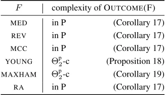
For the judgment aggregation proceduresFthat we con-sidered above, OUTCOME(F) isΘp2-hard. For an overview, see Table 2.
F complexity of OUTCOME(F)
MED Θp2-c (Lang and Slavkovik 2014)
REV Θp2-c (De Haan and Slavkovik 2017)
MCC Θp2-c (Lang and Slavkovik 2014)
YOUNG Θp2-c (Endriss and De Haan 2015)
MAXHAM Θp2-c (De Haan and Slavkovik 2017)
RA ∆p2-c (Endriss and De Haan 2015)
Table 2: The computational complexity of outcome determi-nation for various proceduresF.
Krom and (Definite) Horn Formulas
In this section, we consider the fragments of Krom (2CNF), Horn and definite Horn formulas—for a formal definition of these fragments, see the appendix. These fragments can be used to express settings where only basic dependencies between issues play a role—see Example 2 for an indication.Example 2. Krom (2CNF) formulas can be used to express dependencies of the form “if we decide to use software tool 1 (s1) or software tool 2 (s2), then we need to purchase the
entire package (p):”(s1∨s2)→p≡(¬s1∨p)∧(¬s2∨p).
Definite Horn formulas can be used to express depen-dencies of the form “if we hire both researcher 1 (r1) and
For some judgment aggregation rules these fragments make computing outcomes tractable, and for other judgment aggregation rules they do not. We begin with considering the rulesMEDandMCC. Computing outcomes for these rules is tractable when restricted to Krom formulas, but not when restricted to (definite) Horn formulas.
Proposition? 1. OUTCOME(MED) is Θp
2-hard even when
restricted to the case whereΓ∈DEFHORN.
Proposition? 2. OUTCOME(MCC) is Θp
2-hard even when
restricted to the case whereΓ∈DEFHORN.
The following result refers to the notion of majority con-sistency (see, e.g., Lang and Slavkovik 2014). A profileris
majority consistent(with respect to an integrity constraintΓ) if the majority outcomemr is consistent withΓ. A
judg-ment aggregation procedure ismajority consistentif for each integrity constraintΓand each profilerthat is majority con-sistent (w.r.t.Γ), the procedure outputs all and only those complete ballots that agree with the (partial) ballotmr.
Theorem 3. For all judgment aggregation proceduresFthat are majority consistent, e.g.,F ∈ {MED,MCC},OUTCOME
-(F)is polynomial-time solvable whenΓ∈KROM.
Proof. The general idea behind this proof is to use the prop-erty that when Γ ∈ KROM, the majority outcomemr is
alwaysΓ-consistent. Let(I,Γ,r, s)be an instance of OUT-COME(F) withΓ ∈ KROM. Letr = (r1, . . . , rp). We
con-sider the majority outcomer∗=mr.
We show that the partial ballot r∗ is consistent withΓ. Suppose, to derive a contradiction, thatr∗ is inconsistent withΓ. Then there must be some clause(l1∨l2)of size2
such thatΓ|= (l1∨l2)andr∗sets bothl1andl2to false. By
definition ofr∗, then a strict majority of the ballots inrsetl1
to false, and a strict majority of the ballots inrsetl2to false.
By the pigeonhole principle then there must be some ballotri
inrthat sets bothl1andl2to false. However, sinceΓ|= (l1∨
l2), we get thatridoes not satisfyΓ, which is a contradiction
with our assumption that all ballots in the profile satisfyΓ. Thus, we can conclude thatr∗is consistent withΓ.
SinceF is majority consistent, we know thatF(r) con-tains all ballots that are consistent with both r∗ and Γ. SinceΓ ∈ KROM, deciding ifF(r)contains a ballot that is consistent withscan be done in polynomial time.
We continue with theMAXHAMprocedure for which com-puting outcomes is not tractable when restricted to Krom formulas nor when restricted to definite Horn formulas. Proposition? 4. OUTCOME(MAXHAM) is Θp2-hard even when restricted to the case whereΓ =>.
OUTCOME(MAXHAM) restricted to the case whereΓ =
>coincides with a problem known as CLOSEST STRING for binary alphabets (see, e.g., Li, Ma, and Wang 2002). To the best of our knowledge, this is the first time that the exact complexity of (this variant of) this problem has been identified. OUTCOME(MAXHAM) is also very similar to the problem of computing outcomes for the minimax rule in approval voting (Brams, Kilgour, and Sanver 2004). Corollary 5. OUTCOME(MAXHAM)isΘp2-hard even when restricted to the case whereΓ∈DEFHORN∩KROM.
Finally, we consider the procedureRA, for which comput-ing outcomes is tractable for both Krom and Horn formulas.
Theorem 6. LetCbe a class of propositional formulas (or Boolean circuits) with the following two properties:
• C is closed under instantiation, i.e., for anyΓ ∈ C and any partial truth assignmentα:Var(Γ)→ {0,1}it holds thatΓ[α]∈ C; and
• satisfiability of formulas inCis polynomial-time solvable.
ThenOUTCOME(RA)is polynomial-time solvable when re-stricted to the case whereΓ∈ C.
Proof (sketch). Let C be a class of propositional formulas that satisfies the conditions stated above, and let Γ ∈ C. We can then compute OUTCOME(RA) ={r∗}by directly
using the iterative definition ofr∗given in the description of the ranked agenda procedure. This definition iteratively constructs partial ballotss0, . . . , s2n. Ballots0is the empty
ballot, and for eachi >0, ballotsiis constructed fromsi−1
by using only the operations of instantiating the integrity constraint and checking satisfiability of the resulting for-mula. Due to the properties of C, these operations are all polynomial-time solvable. Thus, constructingr∗=s2ncan
be done in polynomial time.
Corollary 7. For eachC ∈ {KROM,HORN},OUTCOME
-(RA)is polynomial-time solvable when restricted to the case whereΓ∈ C.
An overview of the complexity results that we established in this section can be found in Table 3.
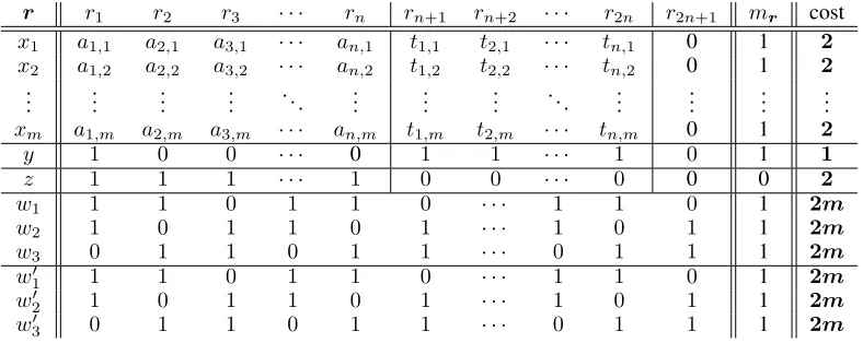
F complexity of OUTCOME(F) restricted to HORN/ DEFHORN
MED Θp2-c (Proposition 1)
MCC Θp2-c (Proposition 2)
MAXHAM Θp2-c (Corollary 5)
RA in P (Corollary 7)
F complexity of OUTCOME(F) restricted to KROM
MED in P (Theorem 3)
MCC in P (Theorem 3)
MAXHAM Θp2-c (Corollary 5)
[image:4.612.351.522.406.567.2]RA in P (Corollary 7)
Table 3: The computational complexity of outcome deter-mination for several procedures F restricted to the case where Γ ∈ KROM, the case where Γ ∈ HORN, and the case whereΓ∈DEFHORN.
The results that we obtained for Horn formulas can all be straightforwardly extended to the fragment of renamable Horn formulas—e.g., the fragment of renamable Horn formu-las satisfies the requirements of Theorem 6. A propositional formulaϕisrenamable Hornif there is a setR⊆Var(ϕ)of variables such thatϕbecomes Horn when all literals overR
Boolean Circuits in DNNF
Next, we consider the case where the integrity constraints are restricted to Boolean circuits in Decomposable Negation Normal Form (DNNF). This is a class of Boolean circuits studied in the area of knowledge compilation. We illustrate how this class of circuits is useful for judgment aggregation.
Knowledge Compilation
Knowledge compilation(see, e.g., Darwiche and Marquis 2002, Darwiche 2014, Marquis 2015) refers to a collection of approaches for solving reasoning problems in the area of artificial intelligence and knowledge representation and reasoning that are computationally intractable in the worst-case asymptotic sense. These reasoning problems typically involve knowledge in the form of a Boolean function—often represented as a propositional formula. The general idea be-hind these approaches is to split the reasoning process into two phases: (1) compiling the knowledge into a different for-mat that allows the reasoning problem to be solved efficiently, and (2) solving the reasoning problem using the compiled knowledge. Since the entire reasoning problem is computa-tionally intractable, at least one of these two phases must be intractable. Indeed, typically the first phase does not enjoy performance guarantees on the running time—upper bounds on the size of the compiled knowledge are often desired in-stead. One of the advantages of this methodology is that one can reuse the compiled knowledge for many instances, which could lead to a smaller overall running time.
A prototypical example of a problem studied in the setting of knowledge compilation is that ofclause entailment(see, e.g., Darwiche and Marquis 2002, Cadoli et al. 2002). In this problem, one is given a knowledge base, say in the form of a propositional formulaϕin CNF, together with a clauseδ. The question is to decide whetherϕ|=δ. This problem is co-NP-complete in general. The knowledge compilation approach to solve this problem would be to firstly compile the CNF formulaϕinto an equivalent expression in a different format. For example, one could consider the formalism of Boolean circuits inDecomposable Negation Normal Form (DNNF)
(orDNNF circuits, for short).
DNNF circuits are a particular class of Boolean circuits inNegation Normal Form (NNF). A Boolean circuitC in NNF is a direct acyclic graph with a single root (a node with no ingoing edges) where each leaf is labelled with>,⊥,x
or¬xfor a propositional variablex, and where each internal node is labelled with∧or∨. (An arc in the graph fromN1
toN2indicates thatN2 is a child node ofN1.) The set of
propositional variables occurring inCis denoted by Var(C). For any truth assignmentα: Var(C) → {0,1}, we define the truth valueC[α]assigned toC byαin the usual way, i.e., each node is assigned a truth value based on its label and the truth value assigned to its children, and the truth value assigned toCis the truth value assigned to the root of the circuit. DNNF circuits are Boolean circuits in NNF that sat-isfy the additional property of decomposability. A circuitC
isdecomposableif for each conjunction in the circuit, the conjuncts do not share variables. That is, for each noded
inCthat is labelled with∧and for any two childrend1, d2of
this node, it holds that Var(C1)∩Var(C2) =∅, whereC1, C2
are the subcircuits ofCthat haved1, d2as root, respectively.
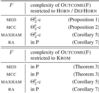
An example of a DNNF circuit is given in Figure 1.
x1 ¬x1 x2 ¬x2
∧ ∧
[image:5.612.367.511.101.150.2]∨
Figure 1: An example of a DNNF circuit.
The problem of clause entailment can be solved in poly-nomial time when the propositional knowledge is given as a DNNF circuit (Darwiche and Marquis 2002). Moreover, every CNF formula can be translated to an equivalent DNNF circuit—without guarantees on the size of the circuit. Thus, one could solve the problem of clause entailment by first compiling the CNF formulaϕinto an equivalent DNNF cir-cuitC(without guarantees on the running time or size of the result) and then solvingC|=δin time polynomial in|C|.
Next, we will show how representation languages such as DNNF circuits can be used in the setting of Judgment Aggregation, and we will argue how Judgment Aggregation can benefit from the approach of first compiling knowledge (without performance guarantees) before using the compiled knowledge to solve the initial problem.
Algebraic Model Counting
We will use the technique of algebraic model counting (Kim-mig, Van den Broeck, and De Raedt 2017) to execute several judgment aggregation procedures efficiently using the struc-ture of DNNF circuits. Algebraic model counting is a gen-eralization of the problem of counting models of a Boolean function that uses the addition and multiplication operators of a commutative semiring.
Definition 1(Commutative semiring). Asemiringis a struc-ture(A,⊕,⊗, e⊕, e⊗), where:
• addition⊕is an associative and commutative binary oper-ation over the setA;
• multiplication⊗is an associative binary operation over the setA;
• ⊗distributes over⊕;
• e⊕ ∈ A is the neutral element of ⊕, i.e., for all a ∈ A,a⊕e⊕=a;
• e⊗ ∈ A is the neutral element of ⊗, i.e., for all a ∈ A,a⊗e⊗=a; and
• e⊕is an annihilator for⊗, i.e., for alla∈ A,e⊕⊗a=
a⊗e⊕ =e⊕.
When⊗is commutative, we say that the semiring is commu-tative. When⊕is idempotent, we say that the semiring is idempotent.
Definition 2(Algebraic model counting). Given:
• a Boolean functionf over a setI of propositional vari-ables;
• a labelling functionλ:Lit(I)→ Amapping literals over the variables inIto values in the setA,
the task of algebraic model counting (AMC)is to compute:
A(f) = M
α:I→{0,1} f(α)=1
O
l∈Lit(I)
λ(l)=1
λ(l).
We can solve the task of algebraic model counting effi-ciently for DNNF circuits when the semiring satisfies an additional condition.
Definition 3(Neutral(⊕, α)). Let (A,⊕,⊗, e⊕, e⊗)be a
semiring, and letλ: Lit(I) → Abe a labelling function for some setIof propositional variables. A pair(⊕, λ)is
neutralif for allx∈ Iit holds thatλ(x)⊕λ(¬x) =e⊗.
Theorem 8(Kimmig, Van den Broeck, and De Raedt 2017, Thm 5). When f is represented as a DNNF circuit, and the semiring(A,⊕,⊗, e⊕, e⊗)and the labelling functionλ
have the properties that (i)⊕is idempotent, and (ii)(⊕, λ)
is neutral, then the algebraic model counting problem is polynomial-time solvable—when givenf andλas input, and when the operations of addition (⊕) and multiplication (⊗) overAcan be performed in polynomial time.
We will use the result of Theorem 8 to show that outcome determination for several judgment aggregation procedures is tractable for the case whereΓis a DNNF circuit. To do so, we will consider the following commutative, idempotent semiring (also known as themax-plus algebra). We letA=
Z∪ {−∞,∞}, we let⊕ = max, ⊗ = +,e⊕ = −∞,
ande⊗ = 1. Whenever we have a labelling functionαsuch that(⊕, λ)is neutral—i.e., such thatmax(λ(x), λ(¬x)) = 0 for eachx∈ I—we satisfy the conditions of Theorem 8.
Theorem 9. OUTCOME(MED) and OUTCOME(MCC) are polynomial-time computable whenΓis a DNNF circuit.
Proof. We prove the statement for OUTCOME(MED). The case for OUTCOME(MCC) is analogous. Let(I,Γ,r, s)be an instance of OUTCOME(MED). We solve the problem by reducing it to the problem of algebraic model count-ing. For (A,⊕,⊗, e⊕, e⊗), we use the max-plus algebra
described above. We construct the labelling functionλas follows. For each x ∈ I, we count the number nx,1 of
ballots r ∈ r such that r(x) = 1 and we count the numbernx,0 of ballots r ∈ r such thatr(x) = 0. That
is, we let nx,0 and nx,1 be the majority strength of ¬x
andx, respectively, in the profiler. We pick a constantcx
such that max{n0
x,0, n0x,1} = 0 where n0x,0 = nx,0 +cx
andn0x,1=nx,1+cx. We then letλ(x) =n0x,1andλ(¬x) =
n0
x,0. This ensures that(⊕, λ)satisfies the condition of
neu-trality (i.e., thatλ(x)⊕λ(¬x) =e⊗for eachx∈ I). This choice of(A,⊕,⊗, e⊕, e⊗)andλhas the property
that the ballotsr∗ ∈ MED(r)are exactly those complete ballotsr∗ that satisfyΓand for which holds thatA(Γ) =
N
l∈Lit(I),r∗(l)=1λ(l). That is, the set MED(r) consists of
those rational ballots that achieve the solution of the algebraic model counting problemA(Γ). We can solve the instance of decision problem OUTCOME(MED) by solving the algebraic model counting problem twice: once forΓand once forΓ[s].
The instance is a yes-instance if and only ifA(Γ) =A(Γ[s]). By Theorem 8, this can be done in polynomial time.
To make this algorithm work for the case of OUTCOME-(MCC), one only needs to adapt the values ofnx,0andnx,1.
Instead of settingnx,0andnx,1to the majority strength of¬x
andx, respectively, we letnx,0 = 0if a strict majority of
ballots r ∈ r have that r(x) = 1, and we let nx,0 = 1
otherwise. Similarly, we let nx,1 = 0if a strict majority
of ballotsr ∈ rhave thatr(x) = 0, and we letnx,0 = 1
otherwise.
Representing the integrity constraint as a DNNF circuit makes it possible to perform more tasks efficiently than just the decision problem OUTCOME(F). For example, the algo-rithms for algebraic model counting can be used to produce a DNNF circuit that represents the setF(r)of outcomes, allowing further operations to be carried out efficiently.
Theorem 10. OUTCOME(REV) is polynomial-time com-putable whenΓis a DNNF circuit.
Proof (sketch). The polynomial-time algorithm for OUT-COME(REV) is analogous to the algorithm described for OUTCOME(MED) described in the proof of Theorem 9. The only modification that needs to be made to make this algo-rithm work for OUTCOME(REV) is to adapt the numbersnx,0
andnx,1, for eachx∈ I. Instead of identifying these
num-bers with the majority strength of¬xandx, respectively, we identify them with the total reversal score ofxand¬x, over the profiler. That is, we letnx,0=Pr∈rsR(r,¬x)and we letnx,1=Pr∈rsR(r, x). For general propositional formu-lasΓ, the reversal scoring functionsRis NP-hard to compute. However, sinceΓis given as a DNNF circuit, we can com-pute the scoring functionsR, and therebynx,0andnx,1, in
polynomial time—by using another reduction to the problem of algebraic model counting. We omit the details of this latter reduction.
Intuitively, the results of Theorems 9 and 10 are a conse-quence of the fact that DNNF circuits allow polynomial-time weighted maximal model computation, and that the judg-ment aggregation proceduresMED,MCCandREVare based on weighted maximal model computation. These results can therefore also straightforwardly be extended to other judg-ment aggregation procedures that are based on weighted maximal model computation.
Other Results
We can extend some previously established results (Proposi-tion 4 and Theorem 6) to the case of DNNF circuits.
Corollary 11. OUTCOME(RA) is polynomial-time com-putable when restricted to the case where Γ is a DNNF circuit.
Corollary 12. OUTCOME(MAXHAM)isΘp2-complete when restricted to the case whereΓis a DNNF circuit.
A similar result forYOUNGfollows from a result that we will establish in the next section (Proposition 18).
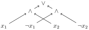
An overview of the results established so far in this section can be found in Table 4.
F complexity of OUTCOME(F)
MED in P (Theorem 9)
REV in P (Theorem 10)
MCC in P (Theorem 9)
YOUNG Θp2-c (Corollary 13)
MAXHAM Θp2-c (Corollary 12)
[image:7.612.90.257.86.184.2]RA in P (Corollary 11)
Table 4: The computational complexity of outcome determi-nation for various proceduresFrestricted to the case whereΓ is a DNNF circuit.
A Compilation Approach
The results of Theorems 9 and 10 and Corollary 11 pave the way for another approach towards finding cases where judgment aggregation procedures can be performed effi-ciently. The idea behind this approach is to compile the integrity constraint into a DNNF circuit—regardless of whether this compilation process enjoys a polynomial-time worst-case performance guarantee. There are several off-the-shelf tools available that compile CNF formulas into DNNF circuits using optimized methods based on SAT solving algorithms (Darwiche 2004; Muise et al. 2012; Oztok and Darwiche 2014b). Since the class of DNNF cir-cuits is expressively complete—i.e., every Boolean function can be expressed using a DNNF circuit—it is possible to compile any integrity constraintΓinto a DNNF circuitCΓ.
The downside is that the circuitCΓcould be of exponential
size, or it could take exponential time to compute it. However, once the circuitCΓis computed and stored in memory, one
can use several judgment aggregation procedures efficiently: MED,MCC,REVandRA.
Thus, this approach restricts the computational bottleneck to thecompilation phase, before any judgments are solicited from the individuals in the judgment aggregation scenario. Once the compilation phase has been completed, there are polynomial-time guarantees on theaggregation phase (poly-nomial in the size of the compiled DNNF circuitCΓ).
CNF Formulas of Bounded Treewidth
The tractability results for DNNF circuits can be leveraged to get parameterized tractability results for the case where the integrity constraint is a CNF formula with a ‘treelike’ structure.
Parameterized Complexity Theory & Treewidth In or-der to explain the results that follow, we briefly introduce some relevant concepts from the theory of parameterized complexity. For more details, we refer to textbooks on the topic (see, e.g., Cygan et al. 2015, Downey and Fellows 2013). The central notion in parameterized complexity is that offixed-parameter tractability—a notion of computational tractability that is more lenient than the traditional notion
of polynomial-time solvability. In parameterized complexity running times are measured in terms of the input sizenas well as a problem parameterk. Intuitively, the parameter is used to capture structure that is present in the input and that can be exploited algorithmically. The smaller the value of the problem parameterk, the more structure the input exhibits. Formally, we considerparameterized problemsthat capture the computational task at hand as well as the choice of pa-rameter. A parameterized problemQis a subset ofΣ∗×N
for some fixed alphabetΣ. An instance(x, k)ofQcontains the problem inputx∈Σ∗and the parameter valuek ∈N. A parameterized problem isfixed-parameter tractablethere is a deterministic algorithm that for each instance(x, k) de-cides whether(x, k) ∈ Qand that runs in timef(k)|x|c,
wherefis a computable function ofk, andcis a fixed con-stant. Algorithms running within such time bounds are called
fpt-algorithms. The idea behind these definitions is that fixed-parameter tractable running times are scalable whenever the value ofkis small.
A commonly used parameter is that of the treewidth of a graph. Intuitively, the treewidth measures the extent to which a graph is like a tree—trees and forests have treewidth 1, cycles have treewidth 2, and so forth. The notion of treewidth is defined as follows. Atree decompositionof a graphG= (V, E)is a pair(T,(Bt)t∈T)whereT = (T, F)is a tree and
(Bt)t∈T is a family of subsets ofV such that:
• for everyv∈V, the setB−1(v) ={t∈T :v∈Bt}is
nonempty and connected inT; and
• for every edge{v, w} ∈ E, there is a t ∈ T such that
v, w∈Bt.
Thewidthof the decomposition(T,(Bt)t∈T)is the number
max{ |Bt|:t∈T} −1. ThetreewidthofGis the minimum
of the widths of all tree decompositions ofG. LetGbe a graph andka nonnegative integer. There is an fpt-algorithm that computes a tree decomposition of Gof widthk if it exists, and fails otherwise (Bodlaender 1996).
Encoding Results We can then use results from the lit-erature to establish tractability results for computing out-comes of various judgment aggregation procedures for in-tegrity constraints whose variable interactions have a tree-like structure. LetΓ = c1∧ · · · ∧cmbe a CNF formula.
Theincidence graph ofΓis the graph(V, E), whereV = Var(Γ)∪ {c1, . . . , cu}andE={ {cj, x}: 1≤j ≤m, x∈
Var(Γ), xoccurs in the clausecj}. Theincidence treewidth ofΓis defined as the treewidth of the incidence graph ofΓ.
We can leverage the results of Theorems 9 and 10 and Corollary 11 to get fixed-parameter tractability results for computing outcomes ofMED,MCC,REVandRAfor integrity constraints with small incidence treewidth.
Proposition 14 (Oztok and Darwiche 2014a, Bova et al. 2015). LetΓ be a CNF formula of incidence treewidthk. Constructing a DNNF circuitΓ0that is equivalent toΓcan be done in fixed-parameter tractable time.
Corollary 15. The problemsOUTCOME(MED),OUTCOME
fixed-parameter tractable when fixed-parameterized by the incidence treewidth ofΓ.
Case Study: Budget Constraints
In this section, we illustrate how the results of the previous section can contribute to providing a computational complex-ity analysis for an application setting. The setting that we consider as an example is that of budget constraints. This set-ting is closely related to that ofParticipatory Budgeting(see, e.g., Benade et al. 2017), where citizens propose projects and vote on which projects get funded by public money. In the setting that we consider, each issuex∈ Irepresents whether or not some measure is implemented. Each such measure has an implementation costcxassociated with it. Moreover, there
is a total budgetBthat cannot be exceeded—that is, each ballot (individual or collective) can set a set of variablesx
to true such that the cumulative cost of these variables is at mostB (and set the remaining variables to false). The in-tegrity constraintΓencodes that the total budgetBcannot be exceeded by the total cost of the variables that are set to true. (For the sake of simplicity, we assume that all costs and the total budget are all positive integers.)
The concepts and tools from judgment aggregation are use-ful and relevant in this setting. This is witnessed, for instance, by the fact that simply taking a majority vote will not always lead to a suitable collective outcome. Consider the example where there are three measures that are each associated with cost1, and where there is a budget of2. Moreover, suppose that there are three individuals. The first individual votes to implement measures1and2; the second votes for measures1 and3, and the third for2 and3. Each of the individuals’ opinions is consistent with the budget. However, taking a majority measure-by-measure vote results in implementing all three issues, which exceeds the budget. (In other words, the individual opinions r1, r2, r3 are all rational, whereas
the collective majority opinionmris not.) This example is
illustrated in Figure 2—in this figure, we encode the budget constraint using a DNNF circuitΓ.
r x1 x2 x3
r1 1 1 0
r2 1 0 1
r3 0 1 1
MAJ(r) 1 1 1
(a) The profiler
x1 x2 ¬x3¬x2¬x1
∧ ∨ ∧
∨
Γ =
[image:8.612.56.285.493.588.2](b) The integrity constraintΓ
Figure 2: Example of an aggregation scenario with a budget constraint (forB = 2andcx= 1for allx∈ I), where the
budget constraint is represented as a DNNF circuitΓ.
Encoding into a Polynomial-Size DNNF Circuit
To use the framework of judgment aggregation to model settings with budget constraints, we need to encode budget constraints using integrity constraintsΓ. One can do this in several ways. We consider an encoding using DNNF circuits
(as in Figure 2b). LetI be a set of issues, let{cx}x∈I be
a vector of implementation costs, and letB ∈Nbe a total budget. We say that an integrity constraint Γencodes the budget constraint for{cx}x∈I andB if for each complete
ballotr :I → {0,1}it holds thatrsatisfiesΓif and only ifP
x∈I,r(x)=1cx≤B.
We can encode budget constraints efficiently using DNNF circuits by expressing them as binary decision diagrams. A
binary decision diagram (BDD)is a particular type of NNF circuit. LetΓbe an NNF circuit. We say that a nodeNofΓis adecision nodeif (i) it is a leaf or (ii) it is a disjunction node expressing(x∧α)∨(¬x∧β), wherex∈Var(Γ)andαandβ
are decision nodes. A binary decision diagram is an NNF circuit whose root is a decision node. Afree binary decision diagram (FBDD)is a BDD that satisfies decomposability (see, e.g., Darwiche and Marquis 2002, Gergov and Meinel 1994).
Theorem 16. For each I, {cx}x∈I and B, we can
con-struct a DNNF circuit Γ encoding the budget constraint for{cx}x∈IandBin time polynomial inB+|I|.
Proof. We construct an FBDD Γ encoding the budget constraint for {cx}x∈I and B as follows. Without loss
of generality, suppose that cx > 0 for each x ∈ I. LetI ={x1, . . . , xn}. We introduce a decision nodeNi,j
for each i ∈ {0, . . . , n} and j ∈ {0, . . . , B}. Take arbi-trary i ∈ {0, . . . , n} and j ∈ {0, . . . , B}. Ifi = n, we let Ni,j = >. If i < n, we distinguish two cases: either
(i)j0 ≤Bor (ii)j0 > B, wherej0 =j+cxi.. In case (i), we letNi,j = (xi∧Ni+1,j0)∨(¬xi∧Ni+1,j). In case (ii),
we letNi,j = (xi∧ ⊥)∨(¬xi∧Ni+1,j). We let the root
of the FBDD be the nodeN0,0—and we remove all nodes
that are not descendants ofN0,0. Intuitively, the subcircuit
rooted atNi,j represents all truth assignments to the vari-ables xi+1, . . . , xn that fit within a budget ofB −j. For
each nodeNi,jit holds that the variables in the leaves reach-able fromNi,jare amongxi+1, . . . , xn. Therefore, we
con-structed an FBDD. Moreover, each complete ballotrsatisfies the circuitΓif and only ifP
x∈I,r(x)=1cx≤B. Thus,Γis
a DNNF circuit constructed in time polynomial inB+|I|
encoding the budget constraint for{cx}x∈IandB.
An example of a DNNF circuit resulting from the en-coding described in the proof of Theorem 16—after some simplifications—can be found in Figure 2b.
Complexity Results
Using the encoding result of Theorem 16, we can establish polynomial-time solvability results for computing outcomes for several judgment aggregation procedures in the setting of budget constraints.
Corollary 17. OUTCOME(MED), OUTCOME(MCC), OUT
-COME(REV), andOUTCOME(RA)are polynomial-time com-putable when restricted to the case where Γ expresses a budget constraint.
For theYOUNGandMAXHAMprocedures, we obtain in-tractability results for the case of budget constraints—for both procedures computing outcomes isΘp2-hard.
Proposition?18. OUTCOME(YOUNG)isΘp
2-hard when
re-stricted to the case whereΓexpresses a budget constraint.
Corollary 19. OUTCOME(MAXHAM)isΘp2-hard when re-stricted to the case whereΓexpresses a budget constraint.
Proof. The result follows directly from Proposition 4.
An overview of the complexity results that we established in this section can be found in Table 5.
F complexity of OUTCOME(F)
MED in P (Corollary 17)
REV in P (Corollary 17)
MCC in P (Corollary 17)
YOUNG Θp2-c (Proposition 18)
MAXHAM Θp2-c (Corollary 19)
[image:9.612.89.258.200.296.2]RA in P (Corollary 17)
Table 5: The computational complexity of outcome determi-nation for various proceduresFrestricted to the case whereΓ is a budget constraint.
Directions for Future Research
In this paper, we provided a set of initial results for restricted languages for judgment aggregation, but these results are only the tip of the iceberg that is to be explored. We outline some directions for interesting future work on this topic.
One first direction is to establish the complexity of OUT-COME(F) for cases that are left open in this paper—for exam-ple, forYOUNGandREVfor the case of Krom and (definite) Horn formulas. Another direction is to pinpoint the complex-ity of OUTCOME(F) for the languages that we considered for other judgment aggregation rules studied in the literature (see, e.g., Lang et al. 2017).
Yet another direction is to extend tractability results ob-tained in this paper—e.g., for Krom and Horn formulas—to formulas that are ‘close’ to Krom or Horn formulas. One could use the notion of backdoors for this (see, e.g., Gaspers and Szeider 2012).
Finally, further restricted languages of propositional for-mulas or Boolean circuits need to be studied, to get a more complete picture of where the boundaries of the expressivity-tractability balance lie in the setting of judgment aggregation. A good source for additional languages is the field of knowl-edge compilation (see, e.g., Darwiche and Marquis 2002, Darwiche 2014, Marquis 2015), where many restricted lan-guages have been studied with respect to their expressivity and support for performing various operations tractably.
Conclusion
In this paper, we initiated the hunt for representation lan-guages for the setting of judgment aggregation that strike a balance between (1) allowing relevant computational tasks
to be performed efficiently and (2) being expressive enough to model interesting and relevant application settings. Con-cretely, we considered Krom and (definite) Horn formulas, and we studied the class of Boolean circuits in DNNF. We studied the impact of these languages on the complexity of computing outcomes for a number of judgment aggregation procedures studied in the literature. Additionally, we illus-trated the use of these languages for a specific application setting: voting on how to spend a budget.
Appendix: Preliminaries
We give an overview of some notions from propositional logic and computational complexity that we use in the paper.
Propositional Logic
Propositional formulas are constructed from propositional variables using the Boolean operators ∧,∨,→, and¬. A
literalis a propositional variablex(apositive literal) or a negated variable¬x(anegative literal). Aclauseis a finite set of literals, not containing a complementary pairx,¬x, and is interpreted as the disjunction of these literals. A formula inconjunctive normal form (CNF)is a finite set of clauses, interpreted as the conjunction of these clauses. For eachr≥
1, anr-clauseis a clause that contains at mostrliterals, and
rCNF denotes the class of all CNF formulas consisting only ofr-clauses.2CNF is also denoted by KROM, and 2CNF formulas are also known asKrom formulas. AHorn clauseis a clause that contains at most one positive literal. Adefinite Horn clauseis a clause that contains exactly one positive literal. We let HORNdenote the class of all CNF formulas that contain only Horn clauses (Horn formulas), and we let DEFHORNdenote the class of all CNF formulas that contain only definite Horn clauses (definite Horn formulas).
For a propositional formulaϕ, Var(ϕ)denotes the set of all variables occurring inϕ. Moreover, for a setX of vari-ables, Lit(X)denotes the set of all literals over variables inX, i.e., Lit(X) = {x,¬x: x ∈ X}. We use the stan-dard notion of(truth) assignmentsα:Var(ϕ)→ {0,1}for Boolean formulas andtruthof a formula under such an as-signment. For any formulaϕand any truth assignmentα, we letϕ[α]denote the formula obtained fromϕby instantiating variablessin the domain ofαwithα(x)and simplifying the formula accordingly. By a slight abuse of notation, ifαis defined on all Var(ϕ), we letϕ[α]denote the truth value ofϕ
underα.
Computational Complexity Theory
We assume the reader to be familiar with the complexity classes P and NP, and with basic notions such as polynomial-time reductions. For more details, we refer to textbooks on computational complexity theory (see, e.g., Arora and Barak 2009).
In this paper, we also refer to the complexity classesΘp2 and ∆p2 that consist of all decision problems that can be solved by a polynomial-time algorithm that queries an NP oracleO(logn)ornO(1)times, respectively. Formally, algo-rithms with access to an oracle are defined as follows. LetO
anOoracleis a Turing machine with a dedicatedoracle tape
and dedicated statesqquery,qyesandqno. WheneverMis in the stateqquery, it does not proceed according to the transition relation, but instead it transitions into the state qyes if the oracle tape contains a stringxthat is a yes-instance for the problemO, i.e., ifx∈O, and it transitions into the stateqno ifx 6∈ O. Intuitively, the oracle solves arbitrary instances ofOin a single time step. The classΘp2(resp.∆p2) consists of all decision problemsQfor which there exists a deterministic Turing machine that decides for each instancexof sizen
whetherx∈Qin time polynomial innby querying some oracleO∈NP at mostO(logn)(resp.nO(1)) times.
LetCbe a class of propositional formulas. The following problem is complete for the classΘp2under polynomial-time reductions whenCis the class of all propositional formulas (Chen and Toda 1995; Krentel 1988; Wagner 1990).
MAX-MODEL(C)
Instance:A satisfiable propositional formulaϕ∈ C, and a variablez∈Var(ϕ).
Question:Is there a model ofϕthat sets a maximal num-ber of variables in Var(ϕ)to true (among all models ofϕ) and that setszto true?
For any classC of propositional formulas, we let MAX-MODEL(C)denote the problem MAX-MODELrestricted to formulasϕ∈ C.
Acknowledgments. This work was supported by the Aus-trian Science Fund (FWF), project J4047.
References
Arora, S., and Barak, B. 2009.Computational Complexity – A Modern Approach. Cambridge University Press.
Benade, G.; Nath, S.; Procaccia, A. D.; and Shah, N. 2017. Preference elicitation for participatory budgeting. InProc. of the 31st AAAI Conf. on Artificial Intelligence (AAAI 2017), 376–382. AAAI Press.
Bodlaender, H. L. 1996. A linear-time algorithm for finding tree-decompositions of small treewidth. SIAM J. Comput.
25(6):1305–1317.
Bova, S.; Capelli, F.; Mengel, S.; and Slivovsky, F. 2015. On compiling CNFs into structured deterministic DNNFs. In
Proc. of the 18th Intern. Conf. on Theory and Applications of Satisfiability Testing (SAT 2015), 199–214.
Brams, S. J.; Kilgour, D. M.; and Sanver, M. R. 2004. A minimax procedure for negotiating multilateral treaties. In
Proc. of the 2004 Annual Meeting of the American Political Science Association.
Cadoli, M.; Donini, F. M.; Liberatore, P.; and Schaerf, M. 2002. Preprocessing of intractable problems. Inf. Comput.
176(2):89–120.
Chen, Z.-Z., and Toda, S. 1995. The complexity of selecting maximal solutions.Inf. Comput.119:231–239.
Cygan, M.; Fomin, F. V.; Kowalik, L.; Lokshtanov, D.; Marx, D.; Pilipczuk, M.; Pilipczuk, M.; and Saurabh, S. 2015.
Parameterized Algorithms. Springer.
Darwiche, A., and Marquis, P. 2002. A knowledge compila-tion map. J. Artif. Intell. Res.17:229–264.
Darwiche, A. 2004. New advances in compiling CNF into decomposable negation normal form. In de M´antaras, R. L., and Saitta, L., eds.,Proc. of the 16th European Conf. on Artificial Intelligence, (ECAI 2004), 328–332. IOS Press. Darwiche, A. 2014. Tractable knowledge representation formalisms. In Bordeaux, L.; Hamadi, Y.; and Kohli, P., eds.,Tractability: Practical Approaches to Hard Problems. Cambridge University Press. 141–172.
Dietrich, F., and List, C. 2007. Arrow’s theorem in judgment aggregation. Social Choice and Welfare29(1):19–33. Dietrich, F. 2007. A generalised model of judgment aggrega-tion. Social Choice and Welfare28(4):529–565.
Downey, R. G., and Fellows, M. R. 2013.Fundamentals of Parameterized Complexity. Springer Verlag.
Endriss, U., and de Haan, R. 2015. Complexity of the winner determination problem in judgment aggregation: Kemeny, Slater, Tideman, Young. InProc. of the 14th Intern. Conf. on Autonomous Agents and Multiagent Systems (AAMAS 2015). Endriss, U.; Grandi, U.; de Haan, R.; and Lang, J. 2016. Succinctness of languages for judgment aggregation. In
Proc. of the 15th Intern. Conf. on the Principles of Knowledge Representation and Reasoning (KR 2016). AAAI Press. Endriss, U.; Grandi, U.; and Porello, D. 2012. Complexity of judgment aggregation. J. Artif. Intell. Res.45:481–514. Endriss, U. 2016. Judgment aggregation. In Brandt, F.; Conitzer, V.; Endriss, U.; Lang, J.; and Procaccia, A., eds.,
Handbook of Computational Social Choice. Cambridge Uni-versity Press, Cambridge.
Gaspers, S., and Szeider, S. 2012. Backdoors to satisfaction. In Bodlaender, H. L.; Downey, R.; Fomin, F. V.; and Marx, D., eds.,The Multivariate Algorithmic Revolution and Beyond, 287–317. Springer Verlag.
Gergov, J., and Meinel, C. 1994. Efficient analysis and manipulation of OBDDs can be extended to FBDDs.IEEE Transactions on Computers43(10):1197–1209.
Grandi, U., and Endriss, U. 2013. Lifting integrity constraints in binary aggregation. Artificial Intelligence199:45–66. Grandi, U. 2012. Binary Aggregation with Integrity Con-straints. Ph.D. Dissertation, University of Amsterdam. Grossi, D., and Pigozzi, G. 2014. Judgment Aggregation: A Primer. Morgan & Claypool Publishers.
Lang, J.; Pigozzi, G.; Slavkovik, M.; van der Torre, L.; and Vesic, S. 2017. A partial taxonomy of judgment aggrega-tion rules and their properties. Social Choice and Welfare
48(2):327–356.
Li, M.; Ma, B.; and Wang, L. 2002. On the closest string and substring problems.J. of the ACM49(2):157–171.
List, C., and Pettit, P. 2002. Aggregating sets of judgments: An impossibility result.Economics and Philosophy18(1):89– 110.
Marquis, P. 2015. Compile! In Bonet, B., and Koenig, S., eds.,Proc. of the 29th AAAI Conf. on Artificial Intelligence (AAAI 2015), 4112–4118. AAAI Press.
Muise, C. J.; McIlraith, S. A.; Beck, J. C.; and Hsu, E. I. 2012. Dsharp: Fast d-DNNF compilation with sharpSAT. In
Kosseim, L., and Inkpen, D., eds.,Proc. of the 25th Canadian Conf. on Artificial Intelligence (Canadian AI 2012), 356–361. Springer Verlag.
Oztok, U., and Darwiche, A. 2014a. CV-width: A new com-plexity parameter for CNFs. InProc. of the 21st European Conf. on Artificial Intelligence (ECAI 2014), 675–680. IOS Press.
Oztok, U., and Darwiche, A. 2014b. On compiling CNF into decision-DNNF. InProc. of the 20th Intern. Conf. on Principles and Practice of Constraint Programming (CP 2014), 42–57. Springer Verlag.
Additional Material: Lemmas and Proofs
As additional material, we provide proofs for all statements in the main paper marked with a star (?), as well as additional lemmas used for these proofs.Lemma 20. MAX-MODEL(3CNF)isΘp2-complete.
Proof. We sketch a reduction from MAX-MODELfor arbi-trary propositional formulas. Let(ϕ, z)be an instance of MAX-MODEL. By using the standard Tseitin transformation, we can transformϕinto a 3CNF formulaϕ0with Var(ϕ0) = Var(ϕ)∪Z for some set Z of new variables, such that for each truth assignment α : Var(ϕ) → {0,1} it holds thatϕ[α]is true if and only if there exists a truth assign-mentβ:Z → {0,1}such thatϕ0[α∪β]is true.
We then transform ϕ0 into a 3CNF formula ϕ00
with Var(ϕ00) =Var(ϕ0)∪Z0, for the setZ0 ={z0:z∈Z}
of fresh variables, such that the maximal models ofϕ00 corre-spond exactly to the maximal models ofϕ. We defineϕ00as follows:
ϕ00=ϕ0∧ ^ z∈Z
((¬z∨ ¬z0)∧(z∨z0)).
Each model ofϕ00then must set the same number of variables inZ∪Z0to true—namely|Z|of them.
Lemma 21. MAX-MODEL(HORN ∩ KROM) is Θp2 -com-plete.
Proof. We give a reduction from MAX-MODEL(3CNF). Let (ϕ, z) be an instance of MAX-MODEL(3CNF), where Var(ϕ) =X ={x1, . . . , xn}and whereϕconsists of
the clausesc1, . . . , cm. Without loss of generality, we may
assume that each clausecj is of size exactly 3. Also, with-out loss of generality, we may assume thatϕis satisfied by the “all zeroes” assignment, that is, by the assignmentα0
such thatα0(xi) = 0for all i ∈ [n]. Moreover, we may
assume without loss of generality thatm≥n. We construct an instance(ϕ0, z0) of MAX-MODEL(HORN∩KROM)as follows.
For each clausecj, we introduce fresh variablesyjuandyuj,`,
foru∈[3]and`∈[n]. Moreover, for eachxi, we introduce
fresh variablesx1i,x0i,z1i,`for`∈[m+ 1]andzi,`0 for`∈
[m]. We then let ϕ0 consist of the following clauses. For eachj∈[m], we add the clauses:
(¬y1
j ∨ ¬y
2
j),(¬y
1
j ∨ ¬y
3
j),(¬y
2
j ∨ ¬y
3
j),
ensuring that at most one variable amongy1
j, y2j, y3j can be
true. Moreover, for eachj ∈[m]and eachu∈[3], we add the clauses:
(yu
j →yj,u1),(yj,u1→yj,u2), . . . ,(yj,nu −1→yuj,n),
(yu
j,n→yju),
ensuring that the variables yu
j andyj,`u get the same truth
value, for eachu∈[3]and eachj∈[m].
Then, for eachi ∈ [n], we add the clause(¬x1
i ∨ ¬x0i),
ensuring that at most one variable amongx1
i, x0i is true.
More-over for eachi∈[n]we add the clauses:
(x1
i →zi,11),(zi,11→z1i,2), . . . ,(zi,m1 →zi,m1 +1), (z1
i,m+1→x1i),
and:
(x0
i →z0i,1),(zi,01→zi,02), . . . ,(zi,m0 −1→z0i,m),
(z0
i,m →x0i),
ensuring that the variablesxui andzi,`u get the same truth value, for eachu∈ {0,1}and eachi∈[n].
Finally, we add the following clauses to ϕ0, for each clausecjofϕ. Letcjbe a clause ofϕ, and letlj,ube theu-th
literal incj, foru∈[3]. Iflj,u=xifor somei∈[n], we add the clause(yju →x1i), and iflj,u =¬xi for somei∈ [n], we add the clause(yu
j →x0i).
To finish our construction, we letz0=x1
i, for the uniquei
such thatz=xi.
Before we show correctness of this reduction, we establish several other properties of the formula ϕ0. Any maximal model ofϕ0sets at leastn(m+ 1) +m(n+ 1) = 2nm+
n+mvariables to true. Since the “all zeroes” assignmentα0
satisfiesϕ, we can satisfyϕ0by setting all variablesx0i, zi,`0 to true, setting all variablesx1
i, zi,`1 to false, and for eachj∈[m]
setting all variablesyu
j, yj,`u to true for someu ∈ [3], and
setting all variablesyu0 j , yu
0
j,` to false for the otheru
0 ∈[3].
This model ofϕ0sets2nm+n+mvariables to true. Moreover, by construction ofϕ0, we know that each model ofϕ0sets at mostn(m+ 2) +m(n+ 1) = 2nm+ 2n+m
variables to true.
By construction of ϕ0, we know that any model ofϕ0
sets variables xu
i, zui,`to true for at mostoneu ∈ {0,1}
for eachi ∈ [n], and that it sets variablesyu
j, yuj,` to true
for at most one u ∈ [3] for each j ∈ [m]. We argue that any maximal model of ϕ0 must set variables xu
i, zi,`u
to true for exactlyone u ∈ {0,1} for each i ∈ [n], and must set variables yu
j, yj,`u to true for exactlyoneu ∈ [3]
for each j ∈ [m]. Suppose that there is some maximal model ofϕ0 that sets all variablesx1i, x0i, zi,`1 , zi,`0 to false, for some i ∈ [n]. Then we know that this model can set at most 2nm+ 2n−2 variables to true. Since m ≥ n, we know that this model cannot be maximal, since there is a model that sets2nm+n+m > 2nm+ 2n−2 vari-ables to true. From this we can conclude that each maximal model ofϕ0 must set variablesxui, zi,`u to true for exactly oneu ∈ {0,1}for eachi ∈ [n]. An entirely similar argu-ment can be used to show that each maximal model ofϕ0
must set variablesyju, yuj,`to true for exactly oneu∈[3]for eachj ∈[m].
Then, for each maximal model α0 of ϕ0, we can con-struct a truth assignment α: X → {0,1}as follows. For eachxi ∈X, we letα(xi) = 1if and only ifα0 setsx1
i to
true, and we letα(xi) = 0if and only ifα0setsx0i to true.
byα0. This is a contradiction with our assumption thatα0
satisfiesϕ0. Therefore, we can conclude thatαsatisfiesϕ. Conversely, for any model α ofϕ we can construct a modelα0 ofϕ0 as follows. For eachi ∈ [n]and eachu∈ {0,1}, α0 sets the variables xu
i, zi,`u to true if and only
ifα(xi) =u. Moreover, sinceαsatisfiesϕ, we know that
for eachj∈[m]there is someuj∈[3]such thatαsatisfies theuj-th literal in clausecj. Then, for eachj ∈ [m]and
eachu∈[3],α0sets the variablesyju, yj,`u to true if and only ifu=uj. It is straightforward to verify thatα0satisfiesϕ0.
We will now argue that there is a maximal model ofϕthat setszto true if and only if there is a maximal model ofϕ0
that setsz0to true.
(⇒)Suppose that there is a maximal modelαofϕthat setszto true. We can then construct a modelα0 ofϕ0, as described above. It is easy to verify thatα0setsz0to true. We argue thatα0is a maximal model ofϕ0. Suppose, to derive a contradiction, thatα0is not a maximal model ofϕ0—that is, there is some modelβ0ofϕ0that sets more variables to true thanα0. Then, as described above, we can construct a modelβ
ofϕfromβ0. It is straightforward to verify thatβsets more
variables inXto true thanα. This is a contradiction with our assumption thatαis a maximal model ofϕ. Therefore, we can conclude thatα0is a maximal model ofϕ0.
(⇐)Conversely, suppose that there is a maximal modelα0
ofϕ0that setsz0 to true. We can then construct a modelα
ofϕ0, as described above. It is easy to verify thatαsetszto true. We argue thatαis a maximal model ofϕ. Suppose, to derive a contradiction, thatαis not a maximal model ofϕ— that is, there is some modelβofϕthat sets more variables to true thanα. Then, as described above, we can construct a modelβ0ofϕ0fromβ. It is straightforward to verify thatβ0
sets more variables in Var(ϕ0)to true thanα0. This is a con-tradiction with our assumption thatα0is a maximal model ofϕ0. Therefore, we can conclude thatαis a maximal model ofϕ.
Lemma 22. OUTCOME(MED) is Θp2-hard even when re-stricted to the case whereΓ∈HORN.
Proof. We give a reduction from MAX-MODEL(HORN). Let (ϕ, z) be an instance of MAX-MODEL(HORN), where Var(ϕ) =X ={x1, . . . , xn}. We may assume
with-out loss of generality that the “all zeroes” assignmentα0 :
X → {0,1}, for whichα0(xi) = 0for alli∈[n], satisfiesϕ.
We construct an instance(I,Γ,r, s)of OUTCOME(MED), withΓ∈HORN, as follows.
We letI =X∪ {yi,j, y0i,j:i∈[n], j∈[3]}. We defineΓ as follows:Γ =ϕ∧V
i∈[n]((yi,1∧yi,2∧yi,3→xi)∧(y0i,1∧
yi,02∧y0i,3→xi)). We define the profiler= (r1, r2, r3)as
shown in Figure 3. Finally, we letsbe the partial ballot that only setszto1.
Clearly, each rational ballotr∗∈ R(I,Γ)must satisfyϕ, sinceΓ|=ϕ. Moreover, to satisfyΓ, each rational ballotr∗
must—for eachi∈[n]—either (i) setxito1or (ii) set at least
one variable amongyi,1, yi,2, yi,3and at least one variable
among yi,01, y0i,2, yi,03 to 0. In case (i), the total Hamming distance to the profilerincreases with3, and in case (ii), the total Hamming distance to the profilerincreases with
at least4. Therefore, the rational ballotsr∗ with minimal cumulative Hamming distance to the profilercorrespond exactly to the models of ϕthat set a maximal number of variablesx∈ X to true. From this it immediately follows that there exists somer∗∈MED(r)that agrees withsif and only if there is a maximal model ofϕthat setszto true.
Proof of Proposition 1 (sketch). We give a reduction from OUTCOME(MED) restricted to the case whereΓ ∈ HORN. Let(I,Γ,r, s)be an instance of OUTCOME(MED) withΓ∈
HORN. Let r = (r1, . . . , rp). Also, let c1, . . . , cm
denote the clauses of Γ. Moreover, suppose that the clauses c1, . . . , cu are non-definite Horn clauses, and that
the clausescu+1, . . . , cmare definite Horn clauses. We
con-struct an equivalent instance (I0,Γ0,r0, s) of
OUTCOME-(MED) withΓ0 ∈DEFHORN, as follows.
Firstly, we letI0=I ∪ {yj,`:j∈[u], `∈[n+ 1]}. We
obtain the definite Horn formulaΓ0fromΓas follows. Firstly, we add the clausescu+1, . . . , cmtoΓ0. Then, for each
non-definite Horn clausecj, withj ∈[u], we add a definite Horn clause(cj∨yj,`)toΓ0for each`∈[n+ 1]. We obtain the
profiler0= (r10, . . . , rp0)fromras follows. For eachi∈[p], we letri0 agree withri on the issues in I. Moreover, for
eachi ∈ [p]and eachx0 ∈ I0\I, we letr0
i(x0) = 0. It is
straightforward to verify that eachr0iis rational.
We firstly show that for each r∗ ∈ MED(r0) and for each j ∈ [u], it holds that r∗ sets all variables yj,` to0. We proceed indirectly, and suppose that this is not the case, i.e., that there is somej ∈[u]such thatr∗ does not set all variablesyj,` to0. We distinguish two cases: either (i) for
all`∈[n+ 1]it holds thatr∗setsyj,`to1, or (ii) this is not the case. In case (i), we know that the cumulative Hamming distance fromr∗to the profiler0is at leastp(n+1). However, the ballotr0such thatr0(x) = 0for allx∈ I0is rational and
has cumulative distance of at mostpntor0. Thus,r∗does not have minimal distance tor0, which contradicts our as-sumption thatr∗∈MED(r0). In case (ii), we know that there exists some`, `0 ∈[n+ 1]such thatr∗setsyj,`to1andyj,`0
to0. Then, we know thatr∗ |=cj, sincer∗ |= (cj∨yj,`0).
However, then modifyingr∗by settingyj,`to0would result in a rational ballot with strictly smaller cumulative distance to the profiler0, which is a contradiction with our assump-tion that r∗ ∈ MED(r0). Thus, we can conclude that for eachr∗∈MED(r0)and for eachj∈[u], it holds thatr∗sets
all variablesyj,`to0.
It is then straightforward to verify that eachr∗∈MED(r0) satisfiesΓ, and that there exists a ballotr∗∈MED(r)such thatsagrees withr∗if and only if there exists a ballotr∗∈
MED(r0)such thatsagrees withr∗.
r xi yi,1 yi,2 yi,3 yi,01 y0i,2 y0i,3
r1 0 1 1 0 1 1 0
r2 0 1 0 1 1 0 1
[image:13.612.329.550.604.661.2]r3 0 0 1 1 0 1 1
Figure 3: The profile r = (r1, r2, r3) in the proof of


![Figure 3: The profile r = (r1, r2, r3) in the proof ofLemma 22—here i ranges over [n].](https://thumb-us.123doks.com/thumbv2/123dok_us/8382447.320968/13.612.329.550.604.661/figure-prole-r-r-r-proof-oflemma-ranges.webp)