INTERACTION
Benjamin Keith Galton-Fenzi
B.
Sc. (Hons Env. Sc.), Grad. Cert. Mar. Sci.
Submitted in fulfilment of the requirements for a
Doctor of Philosophy in Quantitative Marine Science
A joint program between the
Commonwealth Science and Industry Research Organisation and the University of Tasmania
STATEMENT OF DECLARATION
I declare that this thesis contains no material which has been accepted for a degree or diploma by the University or any other institution, except by way of background information and duly acknowledged in the thesis, and to the best of my knowledge and belief no material previously published or written by another persona except where due acknowledgement is made in the text of the thesis, nor does the thesis contain any material that infringes copyright.
This thesis may be made available for loan and limited copying in accordance with the Copyright Act of 1968
Benjamin Keith Galton-Fenzi 2009
ABSTRACT v
ACKNOWLEDGEMENTS vii
LIST OF SYMBOLS ix
CHAPTER 1. INTRODUCTION 1
1.1 Interaction of Ice Shelves with the Ocean 4
1.2 Modelling Ice Shelf-Ocean Interaction 7
1.3 Thesis Aims: Testable Objectives 7
1.4 Thesis Overview 8
CHAPTER 2. ICE-OCEAN THERMODYNAMICS 11
2.1 Ice Shelf-Ocean Dynamics 11
2.2 Frazil Ice-Ocean Dynamics 13
2.3 Concluding Remarks 26
CHAPTER 3. ADAPTATION OF AN OCEAN MODEL 27
3.1 The Regional Ocean Modeling System 27
3.2 The Pressure Gradient Force 28
3.3 Equation of State for Seawater in Polar Regions 40
3.4 Frazil Settling Scheme 41
3.5 Concluding Remarks 44
CHAPTER 4. SIMPLIFIED MODELS OF ICE-OCEAN INTERACTION 45
4.1 The Plume Model of Jenkins & Bombosch (1995) 45
4.2 With Rotation: Variations on Grosfeld (1997) 52
4.3 Concluding Remarks 57
CHAPTER 5. THE AMERY ICE SHELF OCEAN MODEL: SETUP 59
5.1 Geometry and Location 59
5.2 General Model Configuration 68
5.3 Forcing and Initial Conditions 68
5.4 Concluding Remarks 78
CHAPTER 6. THE AMERY ICE SHELF-OCEAN MODEL 79
6.1 General Circulation and Water Mass Properties 79
6.2 Antarctic Bottom Water Formation 85
6.3 Mass Balance of the Amery Ice Shelf 89
6.4 Seasonal Cycles of Melt/Freeze and Circulation 96
6.5 Sensitivity Studies 104
6.6 Concluding Remarks 107
CHAPTER 7. COASTAL ANTARCTIC RESPONSE TO CLIMATE CHANGE 113
7.1 Recent Climate Change 113
7.2 Experiments 116
7.3 Results and Discussion 117
7.4 Concluding Remarks 125
CHAPTER 8. CONCLUSIONS 127
8.1 Summary and Main Findings 127
8.2 Caveats and Future Work 129
APPENDIX 1. EQUATION OF STATE POLYNOMIALS 133
REFERENCES 137
The effect of climate change on the mass balance of ice shelves and bottom water formation is investigated using a terrain-following three-dimensional numerical ocean model. The Regional Ocean Modeling System was modified to simulate the thermodynamic processes beneath ice shelves, including direct basal processes and frazil ice dynamics. Process-orientated studies of simplified ice-shelf-ocean cavities investigate the sensitivity of the melting/freezing to the various parametrisations which describe the internal physics of the models. The Amery Ice Shelf/ocean model is forced with tides, seasonal winds and relaxation to seasonal lateral boundary climatologies. The open ocean surface fluxes are modified by an imposed climatological sea-ice cover that includes the seasonal effect of polynyas.
The circulation and basal melting and freezing show good agreement with glaciological and oceanographic observations that have been collected from beneath the Amery Ice Shelf via boreholes through the ice and in the adjacent area of Prydz Bay. Strong horizontal and thermohaline ("ice-pump") circulation is primarily driven by melting and refreezing of the ice shelf. The net basal melt rate is — 45 Gt year (— 0.7 m year-1), which represents 67 % of the total mass loss of the Amery Ice Shelf. The total amount of refreezing is — 5.3 Gt year-1, of which 70 % is due to frazil accretion. The seasonal variability of the basal melt/freeze (up to ±1 m year-1) within 100 km of the open ocean is the same magnitude as the area-averaged melt rates. The annual averaged bottom water formation rates are r-1.2 Sv to the west of the Amery, in the vicinity of Cape Darnley.
The Amery Ice Shelf/ocean model is used to investigate the sensitivity of the basal melt/freeze and bottom water formation to the inclusion of various physical mechanisms and changes in forcing. Direct comparison with glaciological observations shows that ice-shelf models that include frazil processes improve the simulated pattern of marine ice accretion. Simulations without ice-shelf/ocean thermodynamic processes overestimate bottom water formation by up to 2.8 times as much as simulations with ice-shelf/ocean thermodynamic processes, due to the missing buoyant freshwater from the melting ice shelf. Climate change sensitivity studies suggest that an ocean warming of 1°C above present day temperatures can potentially remove the Amery Ice Shelf in —500 years, solely due to increased basal melting, and can also lead to a significant decrease in the formation of bottom water. This research contributes to understanding how interaction between ice shelves and various forcing mechanisms can lead to changes in basal melt/freeze and dense water formation, which has major implications for the stability of ice shelves, sea level rise, and the salt budget of the global oceans.
ACKNOWLEDGEMENTS
The completion of this thesis would not have been possible without the help of many people. I would like to acknowledge the complementary guidance, inspiration, resources and support of my supervisors Richard Coleman, John Hunter, Simon Marsland and John Church.
I would also like to thank, in no particular order, Claire Maraldi ; Dave Rasch for a great time on the Amery Ice Shelf; Neal Young (ACE CRC); Helen Fricker (Scripps Institution of Oceanography); Hugh Tassell (Geoscience Australia) and Kath McMahon (Macquarie University); Rachael Hurd (ACE CRC) and Mike Craven (AAD); Mark Hemer; Andreas Klocker; Michael Schlodlock (NASA-JPL); Takeshi Tamura and the Hokaido group (Low Temperature Institute, Hokaido); Roland Warner (AAD); Jason Roberts (AAD); Trevor McDougall (CSIRO); Chris Sherwood (USGS); Robin Robertson (ADFA, Canberra); The Society of Sub-professional Oceanographers (SoS0) and last but not least, Ben Joseph (UTas) for fantastic computing support. Special thanks must also go to Benoit Legresy (LEGOS, Toulouse) for hosting me during two visitis to LEGOS; Mike Dinniman (ODU, Norfolk) and Paul Holland (BAS, Cambridge) for allowing me to examine specific parts of their code for development of the model presented here. Thanks also to my examiners Adrien Jenkins (BAS) and Chris Sherwood (UGS) for their constructive comments.
This research was supported by a scholarship jointly provided by the Commonwealth Science and Industry Research organisation and the University of Tasmania as part of the Quantitative Marine Science PhD program, and a stipend from the Antarctic Climate and Ecosystems Cooperative Research Centre. Supercomputing resources were kindly provided by the Tasmanian Partnership for Advanced Computing, Hobart and under two separate grants from the National Computing Infrastructure (formally known as the Australian Partnerships for Advanced Computing) located in Canberra.
I am especially indebted to Bill Scott for sharing with me his love for science. Second last is a thanks to my friend and office mate Andrew Meijers. Finally, to Wenneke ten Hout, my eternal gratitude.
Bedankt, mijn kleine prinsesje
LIST OF SYMBOLS
Latin Symbols
a Slope of liquidus for seawater (Tf decrease with S) ar Aspect ratio of frazil discs
A
Tidal amplitudeA
AreaOffset of liquidus for seawater (Tf at 5=0, z=surface) Freezing temp change with depth (Tf decrease with zeta)
Cd Drag coefficient
c crystal drag coefficient
Cj Specific heat capacity of ice
cto Specific heat capacity of seawater Frazil concentration
Diameter of frazil crystal Kinetic energy
Barotropic Kintetic energy
f' Rate of change of frazil ice volume Tracer flux
Barotropic Kinetic Energy Fraction Acceleration due to gravity
Thickess of a sigma layer He Heaviside function
Total average depth
HC
Haney criteria Ocean heat content Ice draftFrazil size class Thermal conductivity
kT Molecular thermal diffusivity of seawater
ks
Molecular haline diffusivity of seawater Tracer eddy diffusionKx,y Horizontal tracer eddy diffusion
K,
Vertical tracer eddy diffusion Turbulent length scale Latent heat of ice fusion Basal melt ratem* Ratio between frazil radius and Kolmogorov length scale Mass of seawater fraction and frazil
Al Total number of frazil size classes
Nu
Nusselt number
Frazil precipitation rate
Pressure
Pb
Pressure at ice shelf base
Pr
Molecular Prandtl number of seawater
Re Frazil disc reynolds number
qc Rate of conductive heat transfer
qi
Rate of conductive heat transfer from ice to freshwater
Surface heat flux
Radius of major frazil ice surface
Bottomslope
Salinity of mixed layer
Tracer source
Sb
Salinity of boundary layer
Salinity of shelf (salt trapped in ice during freezing)
Sc Molecular Schmidt number of seawater
Sh Sherwood number
Sv Sverdrup
Time
Temperature of mixed layer
Tb
Temperature of boundary layer
Tf
Thermodynamic freezing point temperature
Temperature of ice
Mixed layer velocity
u v Wind speed
Tt, 77,
Depth averaged velocities in the x and y directions
ui Critical erosion velocity at ice shelf base
Friction velocity
Advection velocity
< V > Maximum baroclinic velocity
✓
Volume
terminal velocity
Wturb
Turbulent motions of frazil crystals
x,y
Horizontal coordinates
Greek Symbols
Direction of the axis of principal variability
"YS Salt transfer coefficient at ice shelf base
-rr
Heat transfer coefficient at ice shelf base Salt transfer coefficient for frazil ice Heat transfer coefficient for frazil ice Density of seawaterPa Density of air
P1 Density at the first level of the ocean model
pi Density of ice
Po Reference density of seawater
Ps Density of seawater fraction Stress at ice base or sea floor
a Vertical sigma coordinate
Crinaj Major axis of an ellipse
amin Minor axis of an ellipse
Turbulent dissipation rate (Chapter 2) or Complex error (Chapter 5) Kolmogorov length scale
0 Potential temperature
Basal "two equation" scaling factor 8' Frazil "two equation" scaling factor ii Kinematic viscosity of seawater
Surface stress or Relaxation time (Chapter 3) Tidal phase
CHAPTER ONE
INTRODUCTION
Much of the uncertainty in climate change projections and their impacts on sea level rise and ocean salt budgets is due to limited understanding of the dynamical processes in the cryosphere between grounded ice sheets and the ocean [IPCC, 2007]. Ice shelves are a major part of the global climate system and are an important interface between the grounded ice sheet and the oceans. Most of the snowfall on inland Antarctica drains, via large ice streams, to the sea where it floats seaward of the grounding line forming ice shelves (Fig. 1.1).
About 50% of the Antarctic continental margin [Fox and Cooper, 1994] is framed by ice shelves
kgrn-1Yr1
At 5 6 7 l
9 9
10 [image:11.555.123.459.312.661.2]Log
io
(Ice Flux)
Figure 1.1: Slow moving ice (blue) drains from the Antarctic interior to the coast via fast moving glaciers (red). The image is produced using Lagrangian
balance ice flux estimates from the Arthern et al. [2006] accumulation data set,
2 CHAPTER 1
in coastal embayments, such as the Filchner, Ronne, Ross and Amery, and fringing shelves on the periphery of the ice sheet, such as the Shackleton, Fimbulisen, West, and Larsen shelves (see Fig.
1.2).
Assuming that the Antarctic ice sheet is in approximate steady state, then accumulation over the ice sheet must be balanced by the major outputs. The net average accumulation rate over the Antarctic ice sheet has been estimated at 1811 Gt year-1 [Vaughan et al., 1999], which represents —57 mSv of fresh water that is added to the Southern Ocean. The freshwater contribution is primarily due to melting of ice shelves and the melting of icebergs that have calved from the front of ice shelves. The basal melt water contributions from ice shelves have been estimated using numerical models to be 28 mSv (1 mSv = 103 m3 s —1) of freshwater to the Southern Ocean [Hellmer, 2004]. Earlier estimates of iceberg calving suggest a mass loss of 70 mSv [2016 Gt year-1, Jacobs et al., 1992]. Although these estimates are subject to considerable uncertainty
0
[image:12.562.97.441.315.660.2]180°W
Ablation/Surface-melt Accumulation
...„...--■
===.
Mean Sea LevelGlacier inflow —,-
\
Basal Melting
Marine Ice Accretion
Iceberg calving they imply that the Antarctic continent is currently in negative mass balance. The imbalance of the ice sheet's mass-budget can effect sea level and the heat and salt tracer budgets of the oceans. As such, the ice flux from the major ice sheets into the ocean is strongly controlled by the mass loss processes that occur beneath the ice shelves.
Ice shelves are similarly assumed to be maintained in a dynamic equilibrium that depends on the flow of the feed glacier, snowfall and ablation on the upper surface, basal melting and freezing, and the calving of icebergs (Fig. 1.3).
Figure 1.3: Ice shelf mass balance schematic. Ice shelves are maintained by being in a dynamic balance between the addition of 'ice' via inflowing glaciers, net snow accumulation and marine ice accretion and the removal of ice via basal melting and iceberg calving. The net basal mass loss is equal to the basal melting minus marine ice accretion.
The dynamics (and hence the response time) of upstream inland Antarctic ice is now known to be influenced by ice shelves. Removal of mass from an ice shelf leads to an acceleration and thinning of tributary ice streams and can hence indirectly influence sea level [Dupont and Alley, 2005]. This process is known as the buttressing effect [Thomas, 1979]. For example, Larsen A and B Ice Shelves on the Antarctic Peninsula disappeared in 1995 and 2002 respectively. The collapse of the Larsen B ice shelf and the subsequent speed-up of grounded ice behind [De Angelis and
Skvarca, 2003], led to an increase of about 4 % in the rate of sea level rise [Scambos etal., 2004]. Satellite observations of the Antarctic ice sheet fringing the Amundsen Sea have confirmed that various ice streams there are thinning [ Wingham et al., 2006], accelerating [Joughin et al., 2003], and experiencing retreat of their associated grounding lines, at which the ice stream goes afloat
4
CHAPTER 1
ocean temperature (and hence basal melting) has been implicated in the thinning of Pine Island
Glacier in West Antarctica and the collapse of parts of the Larsen Ice Shelf on the Antarctic
Peninsula
[Shepherd et al.,2003, 2004]. Limitations in our understanding of these processes
present a fundamental barrier to accurate predictions of sea level rise
[JPCC,2007].
The current rate of sea level rise from 1961 to 2003 is about 1.5±0.4 mm yr
-1
[Domingueset al.,
2008]. The contribution due to the melting of continental ice (glaciers, ice caps and ice
sheets) is a substantial source of current sea level rise, and one that is accelerating more rapidly
than was predicted a few years ago. The most recent report from the
IPCC[2007] highlights
that the uncertainty in projections of future sea level rise is dominated by uncertainty concerning
continental ice. Understanding of the key processes that can lead to loss of continental ice must be
improved before reliable projections of sea level rise can be made. The direct basal melting of ice
shelves can also cause a small but significant change in the rate of sea level rise
[Noerdlinger andBrower,
2007;
Jenkins and Holland,2007] due to the density differences between the ice shelf,
primarily composed of glacial ice, and the oceans.
Recent estimates suggest an accelerating mass loss from the Antarctic ice sheet, which is
thought to manifest itself as a freshening signal in the Antarctic bottom water and Antarctic
surface waters. Possible reasons for the Southern Ocean freshening include changes in winds and
precipitation, evolving sea-ice volume, and increased melting of the Antarctic ice sheet
[Jacobs,2004]. Much of the observed freshening in the upper part of the Southern Ocean can be explained
by an increase in net precipitation, north of 60 °S chosen as the southern data limit due to the
low numbers of Argo profiles in the polar region
[Helm,2008]. However, freshening of the deep
ocean near the Antarctic continent can only partially be explained by this mechanism suggesting
the source is due to enhanced ice shelf melt
[Rintoul,2007].
1.1 Interaction of Ice Shelves with the Ocean
In most cases, the major forcing on ice shelf evolution is the basal melt/freeze rate. Ice shelves
largely isolate the ocean below from the effects of the atmosphere. The interaction between the
ice shelves and the ocean is mainly thermodynamic with heat and freshwater exchanged between
the ice shelf and the ocean. The major physical processes of an ice shelf-ocean system are shown
in Fig. 1.4.
The freezing point temperature of seawater decreases with increasing pressure and therefore
depth. Most water that enters ice shelf cavities is either at or near the surface freezing temperature,
such as High Salinity Shelf Water (HSSW). Water masses from the ocean can enter the cavity
and become warmer than the local freezing temperature by moving deeper in the water column.
Interaction of these waters with the base of the ice shelf causes melting. The meltwater can mix
with the ambient water forming Ice Shelf Water (ISW), which is colder than the surface freezing
temperature. Although the ISW is colder, it is fresher and more buoyant than the ambient water
and can rise under the ice shelf. The circulation associated with these processes is known as the
Sea-ice
AABW
Grounding Line
/
Mean Sea Level
Ice Shelf Marine Ice
HSSW
•ISW - " -
‘
Frazil
CDW
Tides
Wind
Polynya
Continental Shelf
Figure 1.4: Schematic of an ice shelf and the 'ice-pump' mechanism (illustrated using the straight and curved lines). An inflow of Circumpolar Deep Water (CDW) can mix with the product of sea-ice formation (solid curved lines), such as High Salinity Shelf Water (HSSW), which can sink (typically poleward) down the continental shelf and can melt the ice sheet. Buoyant freshwater that is released during the melting process rises along the underside of the ice shelf as Ice Shelf Water (ISW) and can become locally supercooled at a shallower depth, leading to the formation of frazil ice (shown by the dots) and basal accretion of marine ice. The water that is created by the re-freezing process is analogous to that created by sea-ice formation (dashed curved lines). These processes are important for deep water formation processes — such as Antarctic Bottom Water (AABW) — that ventilate the abyssal oceans. The grounding line is the region where the ice shelf is in contact with the sea floor.
1.1.1 Marine ice formation
The increase in the local freezing temperature may then cause the ISW to become supercooled where it can freeze directly at the ice shelf base and also (much more effectively) as small frazil ice crystals in the water column that can later accrete to the base of the ice shelf. These two re-freezing processes act to remove the supercooling from the ISW and are important to sub-ice ocean dynamics and overall glacial ice mass balance.
Marine ice has been shown to occupy distinct areas under the Amery Ice Shelf [Fricker et al.,
20011. Recent observations suggest marine ice accretion can act to 'cement' adjacent ice streams
together, thereby enhancing the ice shelf stability [Holland et al., 2009; Craven et al., 2009]. It is thought that a large component of the refrozen marine ice is due to accreted frazil ice. Frazil ice is thought to be important to sub-ice ocean dynamics and overall glacial ice mass balance for a number of reasons described by Smedsrud and Jenkins [2004]:
6 CHAPTER 1
of columnar ice directly onto the ice shelf base
• The presence of suspended ice crystals makes the ISW more buoyant. The formation of
frazil ice thus modifies the forcing on the overturning circulation within the cavity, which
determines the location and rate of marine ice accumulation at the ice shelf base
[Jenkinsand Bombosch,
1995].
With its own set of unique thermal and mechanical properties the presence of marine ice has
important ramifications for the dynamic modelling of ice shelf processes and interaction with
seawater in the ocean cavities beneath them.
1.1.2 Dense water formation
Ocean interaction beneath the ice shelves is important because they are a major component of
the Antarctic mass budget and because they modify the characteristics of the surrounding ocean.
Water that circulates onto the continental shelf is modified through sea-ice formation processes
and interaction with the base of the ice shelves
[Williams et al.,2008]. The resulting dense shelf
water, with sufficient negative buoyancy and an export pathway to the continental slope, can mix
downslope and supply the deep and bottom layers of the global ocean with nutrients and oxygen,
as well as with indicators of recent anthropogenic activity, such as chlorofluorocarbons
[Meredithet al.,
20011 and increased concentrations of carbon dioxide
[Sabine et al.,2004]. Moreover,
the temperature and salinity changes that have been observed for Antarctic water masses may
influence circulation patterns and lead to modification of Antarctic ice shelves
[Jacobs etal.,2002;
Aoki et al.,
2005].
The densest waters in the world's ocean thermohaline circulation are formed in the Southern
Ocean, primarily along the Antarctic continental margin. Several interrelated mechanisms involve
the addition of 'negative buoyancy' by cooling and salinisation of partially ventilated surface and
shelf waters, and by enhancement of mixing with warmer and saltier deep water. Mixing of
modified Circumpolar Deep Water (CDW) near the continental shelf break with locally-formed
HSSW may contribute to the formation of Antarctic Bottom Water (AABW) which is a key driver
in the global thermohaline circulation
[Jacobs,2004]. Heat exchange at the ice-ocean interface
has a major impact on the global ocean heat and freshwater budget as water masses are formed
and modified in the sub-ice shelf cavity
[Wong etal.,1998;
Williams etal.,2001].
Many coupled climate models tend to have too much ventilation of the deep Southern Ocean
[Dutay et al.,
2002]. Perturbation experiments showed that models without ice shelf cavities and
the freshwater flux associated with them both underestimated sea-ice thicknesses and increased
the rate of bottom water formation and overturning
Hellmer[2004]. However, both the formation
1.2 Modelling Ice Shelf-Ocean Interaction
Numerical modelling studies are crucial to improve our understanding of the impact of climate change on floating ice shelves and ice sheet mass balance. Understanding the physical mechanisms between ice shelves and the ocean relies on numerical simulations because observations in the polar regions are logistically difficult. Numerical simulations can also be used to predict the response of these mechanisms to climate change. However, most global climate models poorly resolve the continental shelf surrounding the Antarctic continent. As such, understanding the impacts of climate change on ice-ocean interaction relies on using high resolution regional models.
Three-dimensional numerical ocean models have been applied to cavities under several theoretical ice shelves [Determann and Gerdes, 1994] and more recently with some success to the Filchner-Ronne Ice Shelf [Gerdes et al., 1999; Jenkins and Holland, 2002; Jenkins et al., 2004; Grosfeld et al., 2001; Grosfeld and Sandhager, 2004], the Ross Ice Shelf [Holland et al., 2003], and the Amery Ice Shelf [Williams et al., 2001, 2002]. The local nature of the basal heat and freshwater fluxes are largely understood and can be reasonably well characterised [for example Hellmer and Olbers, 1989; Grosfeld et al., 1997; Holland and Jenkins, 1999]. However, frazil ice dynamics remain a complication to the processes of marine ice formation and the effect of the thermohaline circulation beneath ice shelves.
The dynamics of ISW plumes have been the focus of many specialised modelling studies [for example, MacAyeal, 1985; Hellmer and Olbers, 1989; Jenkins, 1991]. Frazil ice dynamics in ISW plumes have been studied in one-dimensional averaged models by Jenkins and Bombosch [1995]; Sherwood [2000]; Smedsrud and Jenkins [2004] and most recently in two-dimensions by Holland and Feltham [2005]. However, these models are deficient for two reasons: (1) The path that each plume follows must be known beforehand to determine the pressure at the ice shelf base, and (2) the plume is introduced between the ambient fluid and the ice shelf base and so must stay in contact with the base of the ice shelf.
1.3 Thesis Aims: Testable Objectives
8 CHAPTER 1
For this study, a three-dimensional ice shelf ocean cavity model, based on the Regional Ocean Modelling System [ROMS, Shchepetkin and McWilliams, 2005], has been developed, which represents the state-of-the-art in ice shelf cavity ocean modelling. The thesis will apply the ice shelf/ocean model to the Amery Ice Shelf/Prydz Bay system. Since 2002/03 there has been a concerted program of data collection on and under the Amery Ice Shelf and in the adjacent area of Prydz Bay. These data, not available to previous studies, are used to evaluate the model.
As well as for our understanding of the impacts of climate change, understanding the mechanisms that drive the circulation and water mass formation in the vicinity of the MS are important for sediment studies [Hemer and Harris, 2003], biological studies [Craven et al., 2006; Riddle et al., 2007] and paleo-climate studies of past grounding line positions [O'Brien et al., 2007]. Marine ice has been shown to occupy distinct areas under the Amery Ice Shelf [Fricker et al., 2001] which are thought to be important for ice shelf stability [Craven et al., 2009]. Furthermore, some sparse ocean observations suggest that the region is an important source of AABW formation [Yabuki et al., 2006; Meijers et al., 2009]. This is a result of the combined effects of features such as the presence of a large ice shelf cavity, recurring polynyas, and a wide and abruptly sloping continental shelf over which the densest shelf waters in Antarctica are formed [Ohshima et al., 2009].
The objectives of this thesis are summarised as follows:
• To extend the present equations of ice-ocean thermodynamics, including frazil dynamics to be used in a three-dimensional terrain following ocean model.
• To establish the validity of using terrain following models for the study of ice shelf/ocean interaction.
• To quantify the interaction between the ocean and the Amery Ice Shelf with a model that incorporates the physical components outlined in Fig. 1.4. These interactions include describing the general circulation and patterns, and rates of melt/freeze in the vicinity of the ice shelf over a seasonal cycle.
• To make projections about the state of ice shelves and deep water formation under different climate forcing regimes.
1.4 Thesis Overview
The outline of the remainder of this thesis is as follows:
Chapter 2 reviews previous formulations of the thermodynamic processes that occur beneath ice shelves. The chapter identifies some key discrepancies related to frazil ice dynamics that are explored in later chapters.
errors that occur with the pressure gradient force calculation in sigma-coordinate models, due to the non-orthogonality of the vertical coordinate.
Chapter 4 examines the results from some simplified ice shelf ocean cavity studies. The results are evaluated against previous simplified studies, including the Ice Shelf - Ocean Model Inter-comparison Project (ISOMIP) and shows some of the first modelling that includes frazil ice dynamics in a three-dimensional ocean model.
Chapter 5 describes the set-up used for the Amery Ice Shelf ocean model. Particular attention is given to the development of the cavity geometry and seasonal boundary conditions.
Chapter 6 evaluates the response of the Amery Ice Shelf ocean system to present day forcing and tests the sensitivity of some physical parameters.
Chapter 7 tests the sensitivity of the Amery Ice Shelf ocean system to climate change with a range of experiments that examine both the combined and separate effects that changing air-sea forcing and lateral boundary warming can have on the mass balance of the Amery Ice Shelf and the formation of AABW.
Chapter 8 presents the major conclusions of the thesis and discusses some caveats related to using ocean models for ice/ocean interaction studies and briefly discusses the potential for future research.
Two fundamentally different ways are used to evaluate the model, as discussed in the IPCC [2001]. In the first, an attempt has been made to quantify model errors, to consider the causes for those errors (where possible) and to understand the nature of interactions within the model. In the second, the important issues are the degree to which a model is physically based and the degree of realism with which essential physical and dynamical processes and their interactions have been modelled. It should be emphasised that, within this context, evaluation is a more appropriate term than the commonly-used term validation. Validation implies an affirmation that a model is a complete and accurate representation of the system which is being simulated; however, this is impossible in practice, given that such an affirmation requires a complete and accurate understanding of that system [Oreskes et al., 1994].
The evaluation considers:
• Component-level evaluation: the model is evaluated against the results of other models that have contributed to ISOMIP [Hunter, 2006] and against the two-dimensional overturning model first described by Jenkins and Bombosch [1995] in Chapters 3 and 4.
10 CHAPTER 1
CHAPTER
Two
ICE-OCEAN THERMODYNAMICS
The major forcing on ice shelf evolution that is considered here is the melting and freezing processes that occur beneath the ice shelf. Processes that are occur internally to the ice shelf, such as strain thinning and ice shelf calving, are not considered in this thesis. As such, the purpose of this chapter is to develop a set of equations to describe ice-ocean thermodynamics to be used as a basis for the rest of the thesis. The well defined ice shelf-ocean thermodynamics are briefly summarised before a longer review of the current state of frazil ice-ocean thermodynamics. The formulations for the ice-ocean parametrisations that are shown in this chapter are tested in simplified cavities (Chapter 4) and for the Amery Ice Shelf cavity (Chapters 5, 6 and 7).
All known published forms of ice-ocean interactions are derived from Fourier's Law, where the conductive heat transfer rate qc for a given surface area A, is given by [Pitts and Sissom, 1977]:
qc A
w m
-2 (2.1)Here,
R.',
is the temperature gradient in the direction normal to the area A. The thermal conductivity k is an empirically determined constant for the medium, and may depend on other properties such as temperature and pressure. The minus sign in Fourier's law is required by the second law of thermodynamics that is thermal energy transfer resulting from a thermal gradient must be from a warmer to a colder region. Eqn 2.1 is appropriate for ice growth in freshwater and care must be given when examining ice growth rates in saltwater.2.1 Ice Shelf-Ocean Dynamics
At the ice-ocean shelf interface, a parameterisation with a viscous sub-layer model is used (see Fig. 2.1). Three equations represent the conservation of heat and salt and a linearised version of the equation of freezing point of seawater as a function of salinity and pressure [Holland and
Jenkins, 1999]. The free variables that are found by solving the three equations simultaneously are temperature, Tb, salinity, Sb, at the ice shelf base, and the melt rate, m. The parameterization of the fluxes of heat and freshwater that occur at the ice shelf-ocean interface is effective due to the difference in time-scales between the slowly flowing ice shelf (for example, 1 x 10⁻⁵ m s-1-) and the faster sub-ice shelf ocean current (for example, lx 10-1 m s-1). This approach allows the spatial pattern of melting and freezing at an ice shelf base to be simulated. The assumption is that the ice shelf is in a steady-state balance with respect to sources and sinks of mass and heat.
The conservation of heat and salt are:
Pi(L — ciAT)m = pcuryT(Tb — T) (2.2a)
Ud
'YT =
2.12
In(udit 1 v) +
12.5Pr
2
/
3
—9
Ud7s=
2.12
ln(udli 1 v) + 12.5Sc213 9
(2.4a)
(2.4b)
12 CHAPTER 2
Ice shelf
S =O
i
,,,,,,,././ ,././././/7,,/,',//1Viscous sub-layer
Tb=T
f Sb ltdOcean
Figure 2.1: Schematic showing the ice shelf-ocean thermodynamic processes. T and S are the water temperature and salinity, with subscript b indicating the condition at the boundary and subscript i in the ice. The free variables are Tb,
which is the temperature at the ice shelf base, Sb, which is the salinity at the ice
shelf base, and m , which is the melting (m < 0) or freezing Cm > 0) rate (m s'). The symbols are further described in-text.
where, pi
is the density of ice (assumed to be 916 kg m
-3
),
pis the density of ocean water,
Lis the latent heat of ice fusion (3.35 x 10
5
),
ciand
cu,are the specific heats of ice (2009 J kg
-1
K
-1
) and water (3974 J kg
-1
K
-1
), respectively. AT is the temperature difference between the
ice shelf interior, Ti (-20 °C ), and the freezing temperature at the base of the ice shelf,
T1. Tis the temperature and
Sthe salinity of the water away from the base of the ice shelf base. The
assumption is that no salt is present in the ice shelf, which simplifies eqn 2.2b to,
P2Sbm = Prys(Sb — S)
(2.3)
The parameters
-y7,and
7sare coefficients that represent the transfer of heat and salt across the
boundary layer.
Jenkins [1991]used a molecular sub-layer approximation to formulate expressions
for
-y7,and
-ysas:
where, the molecular Prandtl number
(Pr)is the ratio of viscosity to thermal diffusivity and the
molecular Schmidt number
(Sc),is the ratio of viscosity to salinity diffusivity. The kinematic
viscosity of seawater, v (1.95 x 10
-6
m
2
s
-1
), is considered constant
[Holland and Jenkins,1999]
over the thickness of the boundary layer,
h.The friction velocity,
ud,is defined in terms of the
shear stress at the ice-ocean interface:
2 2
FRAZIL ICE-OCEAN DYNAMICS 13
where cd is a dimensionless drag coefficient (0.0025) and u is the velocity of the ocean. Note that the ice is considered to be stationary.
The linearised version of the freezing point of seawater as a function of salinity and pressure is:
TI = aSb b + cP (2.6)
where, T1 is the freezing point at the ice-ocean interface, a is the slope of liquidis for seawater (-5.73 x 10⁻² °C psu-1), b is the offset of liquidus for seawater (8.32 x 10⁻² °C ), c is the change in freezing temperature with pressure (-7.61 x 10⁻⁴ °C dbar-1), and P is the pressure at the ice shelf base.
Eqns 2.2a, 2.3 and 2.6 can be solved simultaneously (using known mixed layer and ice properties) to calculate heat and freshwater (salt) fluxes into the ocean [Scheduikat and Olbers, 1990; Hellmer et al., 1998; Holland and Jenkins, 1999]. This has been done previously for several simulations of the flow beneath ice shelves [for example, Beckmann et al., 1999; Timmermann et al., 2002; Holland et al., 2003]. The calculation of the actual heat and salt fluxes into the top model layer of the ocean includes the meltwater advection term that can be important in long simulations or with high basal melt rates [Jenkins et al., 2001]. Simplifications of these equations can be made by assuming that the melt/freeze rates is only driven by the temperature gradient; that is, by setting S = Sb in eqn 2.2b. This assumption reduces the equations to the "two equation" parametrisation as has been discussed in Holland and Jenkins [1999].
2.2 Frazil Ice-Ocean Dynamics
Frazil is important to sub-ice ocean dynamics and overall glacial ice mass balance for two reasons described by Smedsrud and Jenkins [2004]: (1) Frazil ice growth is thought to be a more effective sink for supercooling than is the growth of columnar ice directly onto the ice shelf base. (2) The presence of suspended ice crystals makes the ISW more buoyant. The formation of frazil ice thus modifies the forcing on the overturning circulation within the cavity, which determines the location and rate of marine ice accumulation at the ice shelf base [Jenkins and Bombosch, 1995].
2.2.1 Fundamental equations
Frazil laden water is considered to be a two-component mixture of ice and seawater that is treated as a homogeneous fluid with spatially-averaged properties. The total mass of frazil ice crystals within a fluid parcel is,
d.A/lc = (dM)C, (2.7)
14
CHAPTER 2
Ps
P = Ps + PC(1—
(2.8)
Pi
where
p,is the density of the seawater without the ice fraction and
pCis the mass of frazil ice per
unit volume of seawater mixture.
There are two ways in which the mass of frazil ice within a seawater parcel can change:
1. There can be sources and sinks of frazil ice mass within the fluid domain due to
melting/freezing, nucleation and precipitation.
2. There can be irreversible molecular or turbulent mixing events that move frazil ice mass
between fluid parcels.
For Boussinesq fluid, the time tendency for frazil concentration takes the form,
C,t
= —V (Cv) — V • (F) + S(2.9)
where the changes to the frazil ice mass can be mathematically represented by the convergence of
tracer flux
Fand tracer source
S.For frazil ice that is suspended in the water column,
Fhas properties that allow for (1) frazil ice
buoyant rising and (2) the turbulent mixing of frazil ice crystals, which yields,
OC OC
-I- V • (Cv) w' —
az =
V
• (KVC) Sut
Advection Mixing Source/Sink
Transient Buoyant rising
(2.10)
where
w'is the vertical buoyancy rising velocity of frazil ice,
zis the vertical coordinate (positive
upwards), and
Kis the turbulent exchange coefficient (eddy diffusivity). The model used for the
majority of the modelling in this thesis is the Regional Ocean Modeling System that allows the
addition of extra tracers, which then handles the advection and diffusion as part of its routines. The
mixing term in eqn 2.10 (first term on R.H.S) is separated into horizontal and vertical components,
such that,
V • (KVC) = V.
(K
x
,
y
V
x
,
v
C
+ KzV ze)(2.11)
The horizontal component K
x
,
y
is not explicit in the model (K
x
=
Ky= 0 m
2
s
-1
), since
the Smolarkiewicz advection scheme used in ROMS is implicitly dissipative
[Shchepetkin andMcWilliams,
1998]. Vertical eddy diffusion for tracers
(Ks)is determined using the K-profile
parametrisation (KPP) by
Large et al.[1994], unless specified to be otherwise.
ROMS solves each term independently using a common numerical technique known as the
"Method of Fractional steps"
[Yanenko,19711. The terms in eqn 2.10 are solved in the sequence:
Ocean
FRAZIL ICE-OCEAN DYNAMICS 15
Melting and freezing
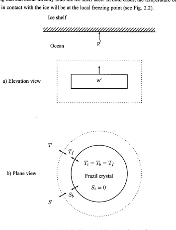
The process of freezing onto ice crystals that are suspended in the ocean is analogous to that of freezing that can occur directly onto the ice shelf base. In both cases, the temperature of the water that is in contact with the ice will be at the local freezing point (see Fig. 2.2).
Ice shelf
a) Elevation view WI
... .. .• • •
b) Plane view
[image:25.554.107.461.143.604.2]• • ...
Figure 2.2: Schematic of a frazil ice crystal showing exchanges of temperature
T and salinity S across the viscous sub-layer, represented by the dotted circle.
The frazil crystal has a vertical settling velocity w' and can precipitate onto the
base of the ice shelf at a rate p'. The system is simplified here by making Sb = 5,
which is analogous to the 'two equation' basal ice-ocean interaction formulation
described in Holland and Jenkins [1999].
16
CHAPTER 2
crystals to surrounding
freshwater(per unit crystal area) from Fourier's Law (eqn 2.1), is:
Nuk
= (Ti — T)
A 1
(2.12)
where
Nu isthe Nusselt number, describing the ratio of total heat transfer to conductive heat
transfer,
k = kTpcp(,-0.564 W m -1 K-1) is the thermal conductivity across the ice-water
interface,
lis characteristic turbulence length scale and
kT— 1.4
x 10-7is the molecular thermal
diffusivity of seawater.
Jenkins and Bombosch
[1995] state that, as the Nusselt number does not vary significantly
from unity, then the transfer of heat from the crystal to the surrounds is solely by molecular
diffusion
[Drazin and Reid,Second Edition, 2004;
Hammar and Shen,1995] 1 . However,
Hollandet al.
[2007] found that the Nusselt number formulation developed by
Hammar and Shen[1995]
incorrectly shows
Nu increasesas the crystal radius decreases, rather than
decreasesas the crystal
radius decreases, once eddies that move heat away from the crystals surface become smaller than
the crystal radius.
Defining an appropriate / is crucial for determining the boundary-layer mixing. The choice of
I
should match the length scale over which the relevant temperature gradient is taken. Previous
authors have chosen a variety of quantities to use for
I.Most authors use the crystal disc radius r
[Daly,
1984;
Hammar and Shen,1995;
Sherwood,2000;
Holland and Feltham,2005;
Smedsrud,2002;
Smedsrud and Jenkins,2004], but the length
V3/8r(based on the crystals total surface
area), the disc thickness and half of the disc thickness
[Jenkins and Bombosch,1995] have
also been used.
Holland et al.[2007] argue that
lis the scale beneath which eddies mix the
frazil crystal's boundary layer rather than moving the crystal; whether any such eddies exist is
established by comparing
Ito the Kolmogorov length scale, ii =
(v/E) 1/4 , where
cis the turbulent
dissipation rate. Using any of the smaller lengths mentioned above will overestimate the influence
of these relatively small eddies on the particles relative velocity and thus underestimate their effect
on mixing of its thermal boundary layer
[Holland et al.,2007].
The formulation of frazil boundary layers in the scientific literature make use of the assumption
that the entire crystal is at the local freezing point: that is, there is a zero internal temperature
gradient between the edge of the crystal in contact with the water and the centre of the crystal (see
Fig. 2.2). However, the analysis is complicated by the fact that the growth and melting of frazil is
influenced by transfer of both heat and salt between the ocean and the surface of the ice crystals.
Three equations
The conservation equations for heat and salt due to frazil ice growth and melting are analogous
to eqns 2.2a and 2.3. With the assumption that heat diffusion into the crystals are negligible
{ 1 + 0.17m Pr1/2 Tri!ir 1
1 > pr 1/2
Nu =
3 1+ 0.55m*213, Pr 11
(2.15)
FRAZIL ICE-OCEAN DYNAMICS 17
(AT = 0) they can be written as:
Pi = Pew -rfrA(Tb — T) (2.13a)
PiSbt = tr/sA(Sb — S) (2.13b)
where, f' is the rate of change of frazil ice volume and the coefficients for heat -6, and salt -y's are defined in terms of the Nusselt Nu and Sherwood Sh numbers, respectively,
NukT
— r , Shks 7.s r
(2.14a)
(2.14b)
where r is the radius of a disk shaped frazil crystal.
The formulas for the exchange coefficients presented here are different to those in previous literature [for example, Jenkins and Bombosch, 1995]. Here, ry's is scaled by the Sherwood number Sh (the mass transfer analogy of the Nusselt number), which is the ratio of turbulent mass transfer to mass diffusion. In the course of this review, it was found that Jenkins and Bombosch [1995] incorrectly scale both
-6,
and -y's only by Nu. Also, the exhange coefficients are scaled by the radius of the frazil disk, r [Holland et al., 2007] and not the half-disk thickness, rar [Jenkins and Bombosch, 1995], where ar is the disk aspect ratio.As such, the growth of frazil ice crystals in saltwater depends on the heat transfer rate that is limited by the rate that salt can move away from the ice crystal and water molecules can move toward the ice crystal. An alternate method of calculating the conservation of heat and salt due to frazil growth/melt might, instead, utilise the Sherwood number to calculate the exchange of water molecules from (to) the face of a melting (freezing) ice crystal.
Here, a version of Nu is used that has been truncated for a reasonable range of crystal radii [Holland and Feltham, 2006; Hammar and Shen, 1995]:
where rrq = 7-171 is the ratio between the frazil radius, r, of size class i and the Kolmogorov length scale, n 1 mm. The Sherwood number can be calculated, utilising the well known mass-heat transfer analogy [Drazin and Reid, Second Edition, 2004], by exchanging Sc for Pr in eqn 2.15, as:
1+ 0.17mSc112 7-4 < sc1
Shi = *s 1/3 1/2
* > 1
1 + 0.55mi213 c mi sc1/2
(2.16)
102
10
18
CHAPTER2
10-2 10-1 100 101
m* = rig
Figure 2.3: Comparing the Nusselt number (Nu; black line) and Sherwood
number (Sh; grey line) over a range of m*, where r 1 mm. The Nu curve is plotted for Pr = 13.8 and the Sh curve is plotted for Sc = 2432. Discontinuities
occur for Nu at m* = 1/Pr1/2 and for Sh at m* = 1/Sc1/2.
and for
Shat m* = 1/Sc
1
/
2
(see Fig. 2.3).
This section has outlined a set of equations (eqns 2.13a-2.16), that together with knowledge
of the local freezing point (eqn 2.6), ambient water properties and the concentrations and size of
frazil already present in the water, can be used to calculate heat and freshwater (salt) fluxes into
the ocean.
Two equations
It is beneficial to reduce the set of equations outlined above to a simpler 'two equation' to
reduce the computational overhead that would be required to solve the set of three equations for
each frazil size class. This section outlines a set of equations describing frazil melt/freeze that have
been implemented into the three-dimensional ocean model used for the remainder of this thesis.
The set of three equations can be simplified by assuming that the growth/melt of frazil ice
is driven purely by the heat exchange; that is,
Sb =
S[for example,
Holland and Feltham,2005;
Smedsrud,2002].
Holland and Feltham[2006] state that since the concern is about the
turbulent transfer of heat, which is much larger than the molecular heat exchange, we can regard
the diffusion of salt and heat to be equal and the possible effects of salinity are therefore negligible.
However, the finite salinity diffusivity supports a salinity difference across the boundary layer and
aSbcp-6
8 = 1
L7's (2.18)
Holland and Feltham [2006] that the boundary salinity is equal to the ocean salinity will lead to melt/freeze rates that are too large.
To correct for the overestimate of frazil melt/growth, Smedsrud and Jenkins [2004] suggested that the Nusselt number can be scaled to consider the effects of salt, based on the scaling factor that was considered for the 'two equation' formulation of the ice shelf-ocean boundary conditions
[Holland and Jenkins, 1999]. That is, as the melt rate of frazil crystals is approximately a linear function of the thermal driving under typical conditions, the impact of salt rejection can be accounted for by simply dividing the heat transfer coefficient, -y,'T by 1.6 to 5.7, depending on the value assumed for the salt transfer coefficient.
However, it has been shown here that the salt transfer coefficient actually depends on the Sherwood number and not the Nusselt number. So, as with the Nusselt number, the exchange of salt between the crystal surface and the ocean scales with the size of the crystal. The ratio of salt transfer coefficient to the heat transfer coefficient is:
Shiks
k N
'TT i 7' (2.17)
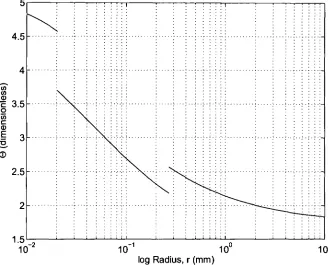
The effect of salt diffusion, as with that for heat is strongly dependant on crystal radii. However, the critical frazil crystal radius that determines the turbulent transition points of heat transfer are different to those for mass transfer with discontinuities at m* = 1/Pr1/2 and m* = 1/Sc1/2. The critical radii can be calculated for m* = r/71 where Ti — 1 mm to occur at the turbulent mass transfer point when r 0.0203 mm and at the turbulent heat transfer point when r 0.2692 mm (Fig. 2.4). The solid horizontal line in Fig. 2.4 is the ratio of salt transfer coefficient to the heat transfer coefficient when Sh = Nu, as is implicit in the forms of the exchange coefficients expressed in Jenkins and Bombosch [1995]. The effect of frazil radii on the exchange of salt and heat between the frazil crystals and the ocean is clear from Fig. 2.4.
Utilising the similarities in the equations between the ice growth rate at the base of an ice shelf and at the surface of an ice crystal, the scaling factor 8 in Holland and Jenkins [1999, eqn 35],
can be modified for frazil to include the formulations of -6 and y's, presented here as,
= 1 aSbcpNuikT
000
LShiks (2.19)
Fig. 2.5 shows the scaling factor for a range of frazil radii, where St, = 34.4. The scaling factor for heat transfer is important across all crystal radii and increases towards smaller frazil radii. Provided this factor is approximately constant, a two equation formulation with an effective transfer coefficient of -6/8' should yield appropriate melt rates.
20 CHAPTER 2
0.035
0.03
0.025 17') En
0.02
:a
0.015co
0.01
0.005
10_i 10° 101
[image:30.562.98.435.89.345.2]Radius, r (mm)
Figure 2.4: The ratio of the salinity ('y's) to thermal (-6) exchange velocities
plotted against a range of frazil ice sizes. -y's and
-6
were calculated using eqns 2.14a and b. Discontinuities occur for frazil radii, when m* = r/n where n ,-- 1 mm, at the turbulent mass transfer point r 0.02 mm and at the turbulent heat transfer point r — 0.27 mm. The solid horizontal line isks/kT = 8 x 10-1044 x 10-7 = 1/175.
The analysis is complicated by the fact that crystal size (and shape) influences the processes of salt and heat transfer, and in reality a spectrum of frazil crystals can exist within the plume at any one time. See Daly [1984] and Morse and Richard [2009] for a more thorough review of the problem. The development of a multiple size class frazil model allows that the source of ice is adjusted for the volume concentration of the i-th class [Smedsrud and Jenkins, 2004; Holland and Feltham, 2005]. The frazil ice concentration C is distributed between N size classes such that:
C
=
Eci
(2.20)Melting and freezing of frazil is modelled by the transfer of a certain number of frazil crystals from class n to the larger size class (n 1) in the case of freezing, or smaller size class (n — 1) in the case of melting. Therefore, the rate change of frazil concentration in each class is determined by the difference in growth (melting) rates between that class and the one above (below). Transfer processes between classes must also be consistent with the movement of the appropriate volume [Smedsrud and Jenkins, 2004].
5
4.5
4
3.5
3 --a
2.5
2
10- 10-i 100
log Radius, r (mm)
1.5 2
[image:31.554.127.455.96.361.2]1
0
1Figure 2.5: Scaling factor plotted against frazil size. The effective exchange based on two equations should include this approximate scaling factor that accounts for the effect of salt.
over the entire crystal. This formulation assumes that the growth of frazil in turbulent seawater only occurs at the edge of the disk and melting occurs over the entire disk to give:
Gi = cp
L°
Nuikt(T1
A =
cpAIukt (Tf T) r] (12arri + 1 )
LAYi ri r i
(2.21a)
(2.2 lb)
In these expressions Nu,, is the turbulent Nusselt number for each size class, i, which is calculated using eqn 2.15, following Holland et al. [2007] and (Yi is calculated using eqn 2.19 for each size class. Note that, for ■CY, = 1, the expressions are those used in previous studies [Smedsrud and Jenkins, 2004; Holland and Feltham, 2005].
Nucleation
Formulations of the melt/freeze of frazil rely on the assumption that the growth and melting of frazil is limited by the turbulent diffusion of heat to and from the area of crystals that are already in the water. So, the first step that is required when the water becomes locally supercooled is to 'seed' the water with a small number of crystals to provide an initial surface area that can be used to calculate the growth rates of ice at the next time-step.
22 CHAPTER 2
and Bombosch, 1995] have all used strategies of introducing a small concentration of frazil ice crystals when the water becomes supercooled. Frazil seeding is due to dendrite-like platelet ice crystals growing on the ice shelf base that may be detached by eddies and suspended in the water column, providing frazil nuclei of various sizes. As such, the seeding process used by these models makes no adjustment to the temperature and salinity when adding frazil seeds to the water column. If a model cell becomes supercooled and does not contain frazil ice crystals, then the concentration of crystals in that cell is set to 10-7, following the strategy of Holland and Feltham [2005]. The assumptions here are:
• There are always sufficient nuclei in the water to grow frazil ice;
• They are distributed evenly over the range of sizes; and
• The initial seed has no impact on the final frazil ice concentrations.
Using a three-dimensional ocean model it is possible that supercooling can occur away from the surface boundary and, as such, frazil nucleation sites are likely at all points in the water column. Seeding is thus allowed to occur at any cell in the model that becomes supercooled.
Secondary nucleation is the process whereby frazil crystals can spawn new "seed" crystals; crystals of the largest size class can fragment into the smallest size class. The main processes thought to give rise to secondary nucleated seed crystals are collisions between frazil and detachment of surface irregularities by fluid shear [Daly, 1984]. The formulation used here follows that outlined in Holland and Feltham [2005] and allows for secondary nucleation process that include turbulent motions to create new seed crystals. The process is limited to produce a maximum number of seed crystals (N = 1 x 10³) [Smedsrud, 2002].
Precipitation, p'
The precipitation of frazil onto the base of an ice shelf borrows from studies of sedimentation in the approach used by Jenkins and Bombosch [1995]. Each frazil size class, i will precipitate at a rate:
2
= 11 w',C (1 — —lul ui2 ) He1 —( 1u12)
\ I (2.22)
where He is the Heaviside function, which prevents erosion from occuring, and ui is a critical velocity above which no precipitation can occur, and zdi is the vertical rise velocity of the frazil crystal (discussed below). This assumes that the flux of crystals that can precipitate out of the water column due to buoyancy is reduced by turbulence in the boundary layer adjacent to the ice shelf base. The critical velocity is expressed as,
2 0.05(p — p2)g2r u, =
Ped (2.23)
critical velocity. The total precipitation rate is,
=
EA
(2.24)2.2.2 Buoyant "terminal" rise velocity, w'
A frazil ice crystal in still water will rise at its terminal velocity when gravitational forces and drag forces are equal. The formulation choice for the rise velocity wb relative to the moving fluid is approximated by the rise velocity for frazil ice in still water, following Holland and Feltham [2005]:
2 4(p — pi)garr wb =
PC1c1
(2.25)
where, c'd is a frazil crystal drag coefficient that is calculated using the Newton-Rhapson method from the disc Reynolds number Re = (wb2r)I v. ed and can be formulated using either of the below equations:
log(c) = 1.386 — 0.892 log (Re) + 0.111 log (Re)2
/ 24 6 +0.4
Re 1 + vRe
(2.26a) (2.26b)
Eqn 2.26a uses an empirical relationship between rise velocity [Gosink and Osterkamp, 1983] and eqn 2.26b is a theoretical formulation of the drag on a sphere [White, 1974]. Note that the calculation of the Reynolds number, and hence drag coefficient is only valid for frazil ice crystals larger than 100 pm.
A recent empirical relationship between frazil size and rise velocity has been devised by Morse
and Richard [2009] based on field observations of frazil ice formation in rivers (sample size = 26470). By fitting power laws to the data they developed a piecewise function:
w
, = 2.025D1'621 ifD < 1.27mm
(2.27) —0.103D2 + 4.069D — 2.024 if 1.27 < D < 7min
where, D = 2r is the diameter of a frazil ice crystal.
_ G083. ar=1/25
_ _ _
G083, a, = 1/15 _ W74, a, = 1/25 _ _ W74, a, = 1/15 _MR09, ar = 1/15• MR09. median
0.25 03 G083, ar=1/25
_ _ _ G083, ar = 1/15 W74, at
=
1/25 0.90.8
0.7
E
0.6To 0.4
.° 0.3
0.2
0.1
0.05 0.1 0.15 0.2 radius, r (mm)
o
o
24
CHAPTER 2
2 3 4 5
[image:34.560.141.383.96.561.2]radius, r (mm)
Figure 2.6: Three different formulations for the frazil rise velocity. The formulations follow Gosink and Osterkamp [1983, blue lines, eqn 2.26a], White
[1974, red lines, eqn 2.26b] and Morse and Richard [2009, black line, eqn 2.27].
2.2.3 Frazil model stability
During the course of this review and the subsequent simulations (see Chapter 4), it became
apparent that a number of stability criterion must be satisfied, which are analogous to the Courant,
Friedrichs, and Lewy (CFL) criterion. These are:
1. Frazil
crystals should not rise vertically through a grid-level in one time-step.
35
30
25
3 20
15
10
5
2. The growth/melt of frazil should not exceed the amount of supercooling/superheating in one time-step, with one related constraint.
3. The amount of frazil that is melted should not exceed the amount of frazil present in the cell; that is, C' = max(0, C AC), where C' is the frazil concentration at an incremented time-step and AC is the amount of frazil melt (negative).
Thermodynamic rate conditions
As melting occurs over the whole surface of a crystal and is therefore much faster than freezing which only occurs at the edges of a crystal, a violation is more likely to occur because of excessive melting rather than excessive freezing. The rate of transfer between size classes due to melting depends on both the surface area, A, of crystals available for melting and the thermal driving, AT. It is difficult to predict the AT or A that will be present in a given model cell before a model is run to be able to 'estimate' the growth-rate and so ensure that the time-step constraint is not violated. Also, the difference between the volumes of the two smallest size classes is the greatest [see eqns 17 and 19, Holland and Feltham, 2006]. During melting the transfer of volume between the classes is proportional to AT(1/r4i — 1/71). The uptake of superheating (in the case of melting) is due (non-linearly) to the difference between size class radii, rather than the radii themselves. So, stability can be enhanced by reducing the difference between the two smallest size classes by increasing the size of the smallest size class, and/or increasing the number of size classes 2•
The violation of this criterion can be avoided by:
1. Using a smaller time-step.
2. Increasing 8 to reduce the frazil growth/melt rates. Given the uncertainty and assumptions with many aspects of our understanding of frazil dynamics, in the context of ice-ocean modelling, 8 represents a parameter that can be used to 'tune' the frazil model.
3. Bound the maximum growth of frazil in one step to a maximum value pre-calculated from AT. The maximum melting of frazil can be bounded by both the limit due to the amount of heat present in the water and the amount of ice that is available for melting.
In the sense of an overall modelling strategy, the time-step ideally needs to be a fraction of the frazil growth and melting. Coupled climate models often use an ice-ocean condition in which only the freezing point at the upper level of the ocean model is diagnosed. At each time-step, the computed temperature is reset to the freezing point and an appropriate amount if ice melted or frozen. In the case of frazil modelling, removing the thermal driving in less than one time-step means that the frazil dynamics is parametrised rather than modelled, which is what is done in most sea-ice models [for example, Schmidt et al., 2004]. However, several time-steps are required during the thermal driving take-up, so that the frazil dynamics can be used to accurately determine


![Figure 2.6: Three different formulations for the frazil rise velocity. The formulations follow Gosink and Osterkamp [1983, blue lines, eqn 2.26a], White [1974, red lines, eqn 2.26b] and Morse and Richard [2009, black line, eqn 2.27]](https://thumb-us.123doks.com/thumbv2/123dok_us/8433828.332585/34.560.141.383.96.561/figure-different-formulations-velocity-formulations-gosink-osterkamp-richard.webp)