Structural Parameterized Complexity
MSc Thesis
(Afstudeerscriptie)
written byJouke E. Witteveen
(born January 28, 1988 in Leeuwarden)
under the supervision ofDr Leen Torenvliet, and submitted to the Board of Examiners in partial fulfillment of the requirements for the degree of
MSc in Logic
at theUniversiteit van Amsterdam.
Date of the public defense: Members of the Thesis Committee: January 28, 2015 Prof Dr Hans L. Bodlaender
Prof Dr Harry M. Buhrman Dr Leen Torenvliet
Contents
1 Introduction 2
2 History 3
3 Preliminaries 5
4 Parameterized Complexity 9
5 Fixed-Parameter Space Tractability 16
6 Two-Part Codes 24
7 Arbitrary Problems Made Tractable 29
8 The Parameter Distribution of VC 34
9 Autoreducibility and XP 41
10 Open Problems 44
11 Conclusion 46
Abstract
1
Introduction
We give an informal introduction to the topics this thesis is concerned with, leaving a formal treatment to the subsequent sections. An overview of the contents of this thesis is provided, so that the reader can skip some or all of the thesis, depending on his/her (current) interests.
Computationally hard problems are an integral part of every day life. The boundary between computationally hard and computationally not hard is a popular area of exploration in computer science. Although computer science has an undeniable presence in society, much of its power is a result of advances in hardware. With computers becoming faster and cheaper, we can take on more and more computational problems. There are computational problems, however, for which making computers faster and more plentiful is of little use. While many such intrinsically intractable problems are known, a definitive separation of the intractable from the tractable is a major unsolved problem in computer science. For a large class of problems known as the NP-complete problems, their presumed intractability is phrased as the statement that they do not lie in a class known asP. A definitive proof of their intractability would settle theP versusNPproblem, which has been troubling computer scientists at least since it was formulated by Cook in 1971.
In the 1990s a more detailed view to the study of tractability and intractabil-ity was introduced. This parameterized take on tractabilintractabil-ity has proven of use for both theoretical and practical computer science. Textbooks have appeared both on the classification of problems in the framework of parameterized complexity and on algorithm design using methods aimed at fixed-parameter tractability. Still, we feel that parameterized complexity has far greater potential then is re-flected in the current body of research.
Most parameterized complexity classes currently studied are derived from the class of problems that are fixed-parameter tractable in a strong sense with respect to computation time. We feel that this leaves us with a rather limited complexity zoo and see an opportunity for the development of more diverse parameterized complexity classes and corresponding notions of preprocessing. In this thesis, we will make a humble beginning with such a diversification by introducing the notion of fixed-parameter tractability with respect to the working memory requirements of computations.
There are also lines of research to which parameterized complexity con-tributes invaluable new methods which have yet to find their way into text-books. One such line of research is that of the distribution of complexity over the instances of problems. Given an intractable problem, one could wonder how many instances are responsible for the intractability of that problem. Using pa-rameter values to keep track of the individual hardness of problem instances, parameterized complexity provides a framework for the analysis of such ques-tions.
of existing insights.
This thesis first works its way to an exposition of some central notions of parameterized complexity in Section 4. While revisiting the basics, we identify some shortcomings in the customary definitions. In Section 5, the definition of fixed-parameter tractability with respect to computation time is lifted into the realm of fixed-parameter tractability with respect to the working memory re-quirements of computations. The main results and contributions of this thesis to parameterized complexity are in Section 6 and Section 7. Section 6 points out a link to descriptive complexity theory which reflects the interpretation of the parameter as a measure of the complexity of problem instances. Section 7 con-tains an investigation of what is needed from a parameter to make an arbitrary problem fixed-parameter tractable. This can be interpreted as an investigation of the limits of the usability of parameterized complexity, or as a foray into the kinds of restrictions that could be placed on parameters. For the sake of comparing our methods to classical methods from probability theory, we stray from our structural ways and present, in Section 8, an analysis of the parameter values of a specific graph problem. Compensating for this digression, a funda-mentally structural approach to parameterized complexity is tried in Section 9, using a form of reducibility as the central concept. Although of very limited success, this approach does inspire one of the conjectures listed in the section on possible future research in structural parameterized complexity, Section 10.
2
History
Parameterized complexity is a young branch of computational complexity the-ory. We give a brief overview of its history and of its motivation. As the history of computer science is well documented [19] and references are readily available, we choose to not clutter the bibliography with references that do not relate to the subject matter of this thesis.
was firmly established andPwas recognized as the complexity class represent-ing tractability. However, by the 1990s this take on tractability had become unsatisfactory for a variety of reasons and in a series of four groundbreaking papers, Downey and Fellows introduced a new standard for tractability: fixed-parameter tractability. This new notion was formalized in the complexity class FPTand accompanied by a suitable notion of reducibility, facilitating the struc-tural study of this new complexity class and its relatives [18]. We will mention some of the most important arguments in favor of fixed-parameter tractability as an approach to tractability.
The use of parameters in the specification of problems makes more fine-grained expressions of complexity possible. With parameters representing met-rics or other aspects of the input to a Turing machine, it is possible give a de-scription of the resource requirements of that machine which incorporates these aspects. Such a description is based not only on the length of the input, but also on the parameters. In particular, a parameterized analysis can distinguish complexities that are indistinguishable when expressed as a function of only the length of the input.
In practice, problems for which no tractable solution is known do not always pose problems. This is mostly due to the fact that not all possible inputs of any given length are equally likely to be encountered. In many practical situa-tions, data tends to be cooperative, save for some relatively small troublesome part. Keeping the size of such a troublesome part fixed and looking at the com-plexity behavior for variable input sizes is precisely the fixed-parameter look at complexity. Thus fixed-parameter tractability promises to give a more realistic account of tractability in practice. From a theoretical perspective, we could say that parameterizing problems allows prior knowledge about values of metrics or of other aspects of problem instances to be taken into account when considering tractability. Thus fixed-parameter tractability is a way to loosen the constraints placed on tractability by the classical notion captured byP.
A related motivation for fixed-parameter tractability comes from the desire to understand sources of intractability. For many problems, intractability is a result of a combinatorial explosion. That is, a search space related to solving such a problem has a size that cannot be bounded by any polynomial in the length of the input to a machine that is supposed to solve the problem. Still, there may be an upper bound, however big, to the size this search space that can be expressed in terms of an aspect of the input instead of in terms of the length of the input. If the length of the input and the aspect are not too strongly correlated, such an upper bound should be thought of as confining the combi-natorial explosion. After all, for some inputs of great length the aspect value may nonetheless indicate a relatively limited search space. This is the case, for example, when the input specifies a rather redundant problem instance. In such cases it is often possible to strip away the redundant parts and reduce an in-stance to its more or less intrinsically hard part. Here, we find a connection between parameterized complexity theory and preprocessing practice. More-over, we notice that parameterized complexity enables an investigation of the distribution of the source of complexity, where this distribution is considered within problems.
which a definition can be found in Section 7. It is an open problem whether or not all NP-complete problems are natural. For parameterized versions of NP-complete problems it is unclear which problems to call natural. In fact, such structural considerations are seemingly underdeveloped in current param-eterized complexity research. Suggestions for conditions that should be satisfied by natural parameterized problems are included in Section 6, but all suggested conditions are unsatisfactory. Either they exclude problems which we would want included, or they allow parameterizations such as those constructed in Section 7, which we would want rejected. Nevertheless some parameteriza-tions are intuitively more natural than others and research in parameterized tractability has commonly focussed on those problems that are natural in an intuitive sense. The alternative program of finding parameterized problems re-lated to a classically intractable problem that are both natural in some sense and have favorable fixed-parameter tractability is rarely attempted. Although several textbooks on parameterized complexity have already appeared and re-sults have found applications outside academia, the field of parameterized com-plexity theory is still in flux and its foundations are not yet set in stone.
3
Preliminaries
We review the small number of basic definitions from computer science that are used in this thesis. None of these definitions is unusual, so the reader familiar with computer science may skip this section.
Conceptually, complexity theory is about the difficulty of problems. In order to attempt a formal study, proper definitions are needed. One of the most common perceptions of a problem in complexity theory [3] is that of a decision problem, which is the type of problem we will define in this section and study in this thesis.
In computer science, analphabet is a finite set and every finite set can serve as an alphabet. A finite sequence of characters of an alphabet is called astring. If Σ is an alphabet, the set of all possible strings ofdcharacters of that alphabet is denoted by Σd. The following notational conventions are used throughout
this thesis.
Definition 1. The natural numbers start at 1. For every natural number n, the set of all possible nonempty strings of at mostncharacters of an alphabet Σ is denoted by Σ≤n. The set of all nonempty finite strings of an alphabet Σ is denoted by Σ+, where the + is known as the Kleene plus operator.
N={1,2, . . .},
Σ≤n=
n
[
d=1
Σd,
Σ+= [
d∈N
Σd.
Note that the unions in the above definition are disjoint. For alln∈N, the following length norm is therefore well-defined on Σ≤n and Σ+.
A subset of Σ+ is called alanguage and comes with its own norm.
Definition 3. Thesize of a languageA⊆Σ+is its cardinality and denoted by
kAk.
We call the empty language,∅, and the full language, Σ+, the trivial
lan-guages. Usually in computer science, Σ+ is extended to include the empty
se-quence and the result of this extension is denoted by Σ?. However, a string of
length 0 is often inconvenient and sometimes even invalidates theorems. In fact, we would at times like the length of any string xto be at least 2, so that |x|c
increases monotonically as a function ofc.
Note that all infinite languages have the same cardinality and there exists a bijective correspondence between any countably infinite set and any infinite language. In specific cases, this correspondence can be of a very practical nature. For instance, a language using one alphabet can be related to a language using another alphabet by encoding the symbols of the one alphabet in fixed-length sequences of symbols of the other. Therefore, the following convention does not limit our results.
Definition 4. Throughout this thesis Σ denotes the binary alphabet, {0,1}, and log denotes the binary logarithm.
Another case of a practical bijection is that of a language corresponding to the Cartesian product Σ+×Σ+. Just mapping an element (x, y) of Σ+×Σ+to
the concatenation ofxandydoes not define a bijection between Σ+×Σ+ and Σ+, as we do not know wherexends andybegins in the concatenation. A proper correspondence can be found by using an intermediate self-delimiting language. A languageA isself-delimiting if for everyx∈Aandy∈Σ+we have that the concatenation ofxandyis not inA. Note that no self-delimiting language of size greater than 1 contains the empty string. A self-delimiting language for which we have a direct bijective correspondence with Σ+ is the language where, for
alld∈N, everyx∈Σd is represented by the string obtained by concatenating
d−1 ‘1’s, a ‘0’ and x. If we call this language A, then we have just defined a correspondence between Σ+×Σ+ andA×Σ+. From the concatenation of the
components of an element ofA×Σ+it is possible to recover the element itself,
thus all such concatenations form a language that is in bijective correspondence toA×Σ+ and thus to Σ+×Σ+. Calling the bijective mapping from Σ+×Σ+
to this language f, the practical use off is demonstrated by the fact that we have|f(x, y)|= 2|x|+|y|, which demonstrates that a well-behaved length norm can be defined on products of languages.
The language corresponding to Σ+×Σ+ just constructed serves as an exam-ple of a language that has aninterpretation of its elements. An interpretation that is possible for all strings is given by a correspondence betweenNand Σ+. Any string of characters of our binary alphabet can be considered to be the bi-nary representation of a natural number: ‘0’ corresponds to 1, ‘1’ corresponds to 2, ‘00’ corresponds to 3, ‘01’ corresponds to 4 et cetera. The representation may appear somewhat strange, but, forn∈N, it is just the customary representation ofn+ 1, dropping the leading ‘1’. This interpretation induces an order on Σ+.
A more general form of correspondence between languages is via language maps.
Definition 5. Alanguage mapfrom a languageAto a languageB is a function
f : Σ+→Σ+ such that, for allx∈Σ+, we havex∈A ⇐⇒ f(x)∈B.
Sometimes, when the meaning is clear from the context, language maps are simply called maps. Language maps form the basis of many-one reductions, which we will simply call reductions in this thesis.
Definition 6. A class of language mapsC is a class ofreductions if we have:
1. for every language, the identity map on that language is inC;
2. for every two maps in C, their composition is inC.
The language maps from a languageAto a languageBin Care denoted by
C(A, B).
The properties of a class of reductions make sure that a class of reductions
C defines a preorderC on all languages: AC B ⇐⇒ C(A, B)6=∅. That is,
the properties of a class of reductions warrant reflexivity and transitivity of the given preorder. When composition of reductions is associative, languages and reductions form a category.
Lacking from the discussion so far, but of paramount importance to com-puter science, is the notion of computability. If any theorem deserves the title of fundamental theorem of computer science it would be that the class of com-putable functions is largely invariant under the choice of a formalism for the underlying notion of computability. This theorem is the result of the Church– Turing thesis when the Turing machine, or any other equivalent formalism, is taken as the defining formalization of computability. The prominent formaliza-tion of computability in this thesis will be a form of pseudocode that we consider self-explanatory and for which we will not define an interpreter. We will call a, possibly partial, functioncomputable if there is an algorithm specified in our pseudocode that computes it.
Definition 7. Analgorithm, orprocedure is any computable function or spec-ification thereof according to some formalization of computability.
Thus, there are two kinds of equivalence of algorithms: an extensional one based on their behavior as a function and an intensional one based on their specification.
On inputs where a procedure does not terminate, the corresponding com-putable function is not defined. However, for our purposes we mostly look at resource bounded computations, in which case we may assume procedures terminate on all possible inputs. Therefore, we may assume that all resource bounded computable functions are total functions.
We will be especially interested in decision procedures.
Definition 8. An algorithmf : Σ+→ {true,false} decides membership of a
string x∈Σ+ in a languageA if we have:
f(x) = (
true ifx∈A
An algorithm is adecision procedure if it decides membership of all strings
x∈Σ+ inA.
Any language for which there is a decision procedure is calleddecidable and the membership question for a string in a decidable language is called adecision problem. Slightly abusing terminology, we adopt the following definition.
Definition 9. Aproblem is a language that admits a decision procedure.
Computability and decidability are related and generally the termrecursive is used to designate the overarching concept, but we will not do so here. When it comes to computability or decidability we are interested in the amount of some resource required by the computation involved. In particular, we are interested in the time and space usage of a computation. Here, time usage stands for the number of atomic computational steps that a computation is made up of. Space usage stands for the longest length of the specification of the input-dependent state encountered during a computation. That is, space usage is about the memory requirement of a computation. We will say a procedure is computable in timetto indicate that computation of the procedure terminates after no more thant atomic computational steps. Similar phrases will be used for the decidability of languages instead of computability of procedures and for space instead of time. When we focus on the behavior of resource usage more than on the specifics, we will make use ofO-notation. Letf andgbe functions from an arbitrary domain A to N. In a context where we have an implicit abstraction over a variable xin A, we say thatf(x) is in O(g(x)) if there is a constant csuch that for all but finitely many xinA we havef(x)≤cg(x). In this thesis, c can always be chosen so that the inequality holds for allxin A. We will often use implicit function definitions in place of f and g. Thus, for example, the phrase ‘the elements (x, y) of a languageAare such that|x|is in
O(y2)’ comes to mean the same as the logical expression
∃c:∀(x, y) : (x, y)∈A =⇒ |x| ≤cy2.
Even more specifically, withf mapping (x, y) to|x|andgmapping (x, y) toy2,
the phrase means the same as the expression
∃c:∀(x, y) : (x, y)∈A =⇒ f(x, y)≤cg(x, y).
Similarly, a decision procedure taking input x is said to decide a problem in space O(s(|x|)) if there is a constant c such that for all x ∈ Σ+ the space
used by the decision procedure is at mostcs(|x|). A special phrase is used for procedures taking inputxfor which there is adthat does not depend onxsuch that the time or space usage of the procedure is inO(|x|d). Such procedures are said to be computable in polynomial time or space. We want to emphasize that
O-notation is about functions, not about specific function values. Our choice of notation is motivated by the fact that for the implicit specification of functions it is convenient to be able to refer to function arguments.
As a running example of a problem, in this thesis we will look at the vertex cover problem on simple graphs.
Simple graphs can be visualized by depicting the vertices as dots and drawing lines between related vertices. BecauseEis anti-reflexive, no line will be drawn from a dot directly to itself.
Definition 11. Given a graph (V, E), a subset V0 of V is a vertex cover of (V, E) if for every (v1, v2)∈E we havev1∈V0 orv2∈V0. Thesize of a vertex coverV0 is the cardinality ofV0.
Thevertex cover problem is the language of pairs of a simple graph (V, E) and a natural number k such that there is a vertex cover of size at most k in (V, E). Note that there are countably many pairs of a simple graph and a natu-ral number, so there indeed exists a language admitting such an interpretation. It is not known whether the vertex cover problem is decidable in polynomial time. In fact, it is complete for the complexity class NP of problems that are computable in polynomial time for a formalization of computability that in-cludes nondeterminism. Here, completeness is taken with respect to polynomial time reductions known as Karp reductions. Related to the vertex cover prob-lem is the minimum vertex cover problem, which asks whether a numberk is the smallest possible size of a vertex cover in a graph. For the minimum vertex cover problem it is not even known whether it is in NP. It is, precisely when NPequals the classco-NP of problems of which the complement is inNP.
4
Parameterized Complexity
A structural outline of fixed-parameter tractability is given. On the way, we identify some flaws in the textbook treatments and correct them. The interplay between several concepts that play a central role in the field of parameterized complexity theory is explored.
As with all interesting complexity classes, there is a multitude of ways in which the classes relevant for analysis in parameterized complexity research can be defined. Characterizations of the classical NP include those via non-deterministic Turing machines, via certificates and verifiers, and via reductions and complete problems. Similarly, we will provide several approaches to the classes most important for this thesis.
Before we do so, some attention needs to be given to the concept of a param-eterized problem. For this concept, like for many in paramparam-eterized complexity theory, different definitions exist. In this thesis, we will go with the one intro-duced originally by Downey and Fellows [13, 14].
Definition 12. Aparameterized problem is a subset of Σ+×Σ+. For (x, k)∈
Σ+×Σ+ we callxtheinstance andktheparameter. The parameter is usually interpreted as a natural number.
Throughout this thesis,xandkwill denote arbitrary instances and param-eters of the problems in scope. For convenience we set |x|to twice the number of characters inx.
the length ofxand as our definition is linear in the number of characters such behavior is retained: it is present in terms of the number of characters precisely if it is present in terms of|x|. Thus the main consequence of our choice is that our mathematical expressions can become more elegant than when we would have set|x|to just the number of characters inx. Furthermore, our choice has a technical interpretation. Since we are dealing with the product Σ+×Σ+, we
may need to make x self-delimiting in any practical coding scheme. Ifx has
n characters, this is easily possible in 2n characters by prepending n−1 ‘1’s followed by a ‘0’ tox.
Definition 12 was originally also used by by Flum and Grohe [17], although for their book on parameterized complexity theory [18] they used an alternative definition. In their case a parameterized problem is a subset of Σ+ equipped with a parameterization functionκ: Σ+→
Nthat is computable in polynomial time. The only difference with our definition is that in our case the length of the parameter is not echoed in the length of the instance. This matters in particular when the parameter is not computable from the instance in polynomial time. In such a case, the precise dependency of an algorithm’s complexity on the length of the instance can be obscured by the presence of a specification of the parameter in the instance. Thus, for Flum and Grohe parameters are necessarily internal to the problem. By contrast, our definition allows parameters to capture external knowledge.
When dealing with parameterized problems, it is often desirable to look at fixed-parameter values, giving rise to slices of the problem.
Definition 13. Thekthslice of a parameterized problemA is the problem
Ak={x|(x, k)∈A}.
The class of parameterized problems of which the slices are inP is known as slice-wiseP, or XP[14, 18] and comes in several guises.
Definition 14. A parameterized problem Ais in the class nonuniform XPif there are functions g, e : Σ+ → N and a family of decision procedures, Φ =
{φk}k∈Σ+such that for eachkthe sliceAk is decided byφk in timeg(k)|x| e(k)
. IfAis in nonuniformXPby a decidable (without resource bounds) family Φ, then it is inuniform XP. In this case, we use Φ to indicate the computable mapping k 7→ φk. Indeed, an indexed family is decidable precisely when the
mapping of index values to their corresponding elements is a computable func-tion.
IfAis in uniformXPby someg, e,Φ such thatgandetoo are computable, then it is in strongly uniform XP. When used without modifiers, XP means strongly uniformXP.
The freedom in the choice ofein the definition ofXPmakesXP-algorithms impractical in general. The proper way to stretch the notion of tractability beyond P into the class of fixed-parameter tractable problems, or FPT is a further restriction.
Definition 15. Wheneis taken as a constant in the definitions of the various versions of XP, we obtain the definitions fornonuniform FPT,uniform FPT, andstrongly uniform FPT.
It may seem as if an even stronger notion of tractability is attained by also restricting the effect of g to be additive instead of multiplicative. It turns out, however, that this would lead to the same classFPT. This is a nice robustness property of FPT.
Lemma 1. Let Abe a parameterized problem. The following are equivalent.
1. Ais in FPT.
2. There is a decision procedure that, for some computable function g and constantc, decidesAin time g(k)|x|c.
3. There is a decision procedure that, for some computable function g0 and constantc0, decidesAin time g0(k) +|x|c0.
Proof. The equivalence 1 ⇐⇒ 2 we get because the decidable families of decision procedures for slices ofAand the decision procedures forAare related by uncurrying and currying.
The implication 2 =⇒ 3 follows by takingg(k) =g0(k) + 1 andc=c0, for then we haveg(k)|x|c ≥g0(k) +|x|c0. The opposite direction, 2 ⇐= 3, follows by takingg0(k) =g(k)c+1andc0=c+ 1. As eitherg0(k) or|x|c0 is bigger than
g(k)|x|c, their sum certainly is.
We remark that the above lemma and proof would be invalid if the empty string, which has length 0, was allowed as an instance. Unfortunately, param-eterized problems are commonly defined as subsets of Σ?×Σ? [16, 18] so the
empty string oftenis allowed.
A direct consequence of the definition of FPT is that FPTis a subset of XP. To see that it is a strict subset, we turn to the following problem.
Problem (PPAcc). Parameterized polynomial time acceptance.
We define problems by a membership criterion based on an interpretation of the instance and the parameter.
Instance: x.
Parameter: (φ, e), whereφis a decision procedure andea natural number.
Criterion: φacceptsxin time|x|e.
We claim that this problem is inXPbut not inFPT.
Lemma 2. PPAcc∈XP.
Proof. By standard results in simulation via efficient universal Turing machines [3], we know that for somec it is possible to computeφ(x) from a specification ofφandxin timeO(|x|ce), where the hidden constant depends on the number of states and tapes used byφ. These numbers can be computed fromφ, hence
PPAccis in strongly uniform XP.
Proof. It suffices to show thatPPAccis not inFPT. Suppose for contradiction that it is. Then, for somec there exists a g such that regardless ofφthe slice
PPAcc(φ,c+1)is decidable in timeg(φ, c+1)|x|
c
. However, by the time hierarchy theorem [3], there exists a slice with a decision procedure φ that runs in time
|x|c+1, but is outsideO(|x|c), contradicting our assumed decidability.
An eminent problem that is not known to be tractable in the classical sense is the vertex cover problem. The vertex cover problem might not be inP, but definitely is inFPT, so tractable when parameterized. In fact, the parameter-ized vertex cover problem is a standard example of a fixed-parameter tractable problem.
Problem (VC). Vertex cover.
Instance: G, a simple graph.
Parameter: k, a natural number.
Criterion: Gcontains a vertex cover of size at mostk.
Membership of FPTfollows directly from a simple algorithm by Sam Buss [6, 14, 18] which we include here as Algorithm 1. In the algorithm, the time needed by loop 1 is quadratic inkVkand the time needed by loop 2 is determined by kV0k, which is upper bounded by a function of the parameter. Therefore, the algorithm indeed proves thatVCis in FPT.
Algorithm 1AnFPT-algorithm forVC. Input: A graph (V, E) and a parameterk
Output: The presence of a vertex cover of size kin (V, E) V0← ∅
k0←k
for allv inV do // loop 1
d←the degree of v
if d> kthen //v is necessarily in every cover smaller thank
k0←k0−1
else if d>0 then //v cannot be ignored V0←V0∪ {v}
end if end for
E0←E∩(V0×V0)
if kE0k ≤k0k then // a cover of size k0 might be possible for allsubsets,W, ofV0 of size min(k0,kV0k)do // loop 2
if W is a vertex cover of E0 then return true
end if end for end if return false
input that has been rid of any trivial parts. More generally, it is the goal of preprocessing to identify the intrinsically hard part of the input.
In Algorithm 1, the preprocessing is of a special kind. Because the size of the result of the preprocessing can be upper bounded by a function of the parameter, we have a clean cut in the variables the time needed in both loops depends upon. For the preprocessing, loop 1, the required time is polynomial in the size of the instance, whereas an upper bound on the time required by loop 2 can be determined solely on the basis of the parameter. This kind of preprocessors is called kernelization.
Definition 16. A language map from one parameterized problem to another, mapping (x, k) to (x0, k0), is a kernelization if there is a constant c, and a computable, non-decreasing functionh:N→Nsuch that we have:
1. (x0, k0) is computable in time|x|c;
2. |x0| ≤h(k) andk0 ≤h(k) hold.
We call (x0, k0) thekernel of (x, k). A parameterized problemA iskernelizable if there exists a kernelization fromAto itself.
In our case, loop 1 of Algorithm 1 constitutes a kernelization fromVC to itself, showing thatVCis kernelizable.
Usually the running time of the language map in the definition of kerneliza-tions is allowed to depend on the parameter [6, 16, 18], but this is not necessary for the fundamental lemma about kernelizability.
Lemma 4. Also equivalent to the statements in Lemma 1 is the following.
4. Ais decidable and kernelizable.
Proof. For 3 ⇐= 4, observe that computing the kernel followed by deciding the kernel, the size of which is bounded by a function, h, of the parameter, takes|x|c+g(h(k)) time, wheregis a bound on the running time of the decision procedure. As gandhare both computable, their composition is too.
The 2 =⇒ 4 direction is a bit more involved. In caseA=∅orA= Σ+×Σ+
we can get away with a kernelization mapping all inputs to an arbitrary string. In all other cases we can take some y ∈A and n /∈ A. Let φbe the assumed decision procedure that runs in time g(k)|x|c. We define a kernelization using
φ,y andnas follows. Input: (x, k)
Output: a kernel of size max(|y|,|n|, g(k) +|k|) run φon (x, k) for|x|c+1 steps
if φhas terminatedthen
return y ornaccording to the output ofφ
else
return (x, k) end if
Unfortunately, kernelizations in general are no reductions, so we cannot di-rectly extract a preorder on problems from them. Kernelizations fall short of being reductions in that the identity map is not necessarily admitted. In Sec-tion 7 we will see that it is natural for the length of instances to grow unbounded given a parameter value. Therefore, it is natural for the identity map to violate requirement 2 of Definition 16, |x| ≤h(k), for somex. Nevertheless we are in-terested in a reduction that somehow relates to parameterized problems and in particular toFPTandXP. The proper notion is that of fpt-reductions.
Definition 17. A language map from one parameterized problem to another, mapping (x, k) to (x0, k0), is an fpt-reduction if there are constants c, d, and computable, non-decreasing functionsg, h:N→N, such that we have:
1. (x0, k0) is computable in timeg(k)|x|c;
2. |x0| ≤ |x|d andk0≤h(k) hold.
The difference between fpt-reductions and kernelizations is subtle but im-portant. Additionally, looking at Definition 14 and Definition 15 it should be obvious that fpt-reductions are the most restrictive of several similar types of reductions, the least restrictive of which being nonuniform xp-reductions. Of-ten, results can be readily rephrased in terms of another reduction, but we will stick to fpt-reductions in this thesis.
The definition of fpt-reduction above is not standard, but it is correct.
Theorem 5. The language maps that are fpt-reductions are reductions. More specifically, the identity map is an fpt-reduction and the class of fpt-reductions is closed under composition.
Proof. We will present a proof only of the last statement. Let f1 and f2 be fpt-reductions of signatures that admit the compositionf2◦f1. We will subscript all auxiliary symbols from the definition according to the map they belong to.
1. The compositionf2◦f1 is computable in timeg1(k)|x|c1+g2(k0)|x0|c2 ≤
g1(k)|x|c1+g2(h1(k))|x|d1c2. Hencef2◦f1is computable in timeg(k)|x|c,
withc=c1+d1c2 andg(k) =g1(k) +g2(h1(k)).
2. For f2(f1(x, k)) = (x00, k00), we find |x00| ≤ |x0|
d2 ≤ |x|d1d2 and k00 ≤
h2(k0)≤h2(h1(k)). Hence|x00| ≤ |x|
d
andk00≤h(k), with d=d
1d2 and h=h2◦h1.
Standard definitions [14, 18] omit the first part of requirement 2 of Defini-tion 17, |x0| ≤ |x|d. However, this requirement is essential for Theorem 5. In the classical setting of Karp reductions the bound on the size of the result of the reduction was not necessary because it was implied by the bound on the computation time. With fpt-reductions, though, the computation time may de-pend on the parameter and the bound on the size of the result of the reduction must be made explicitly.
Lemma 6. Also equivalent to the statements in Lemma 1 and Lemma 4 is the following.
5. Ais fpt-reducible to every nontrivial parameterized problem.
Proof. For 2 ⇐= 5, consider the singleton parameterized problem{y}and let
f be an fpt-reduction to{y}, which exists by assumption. We define a decision procedure forAas follows.
Input: (x, k)
Output: true orfalse, consistent with (x, k)∈A
if f(x, k) =y then return true else
return false end if
Computingf(x, k) is possible within the time bound of an acceptable decision procedure, as is testing for equality to the constant y. Hence, this decision procedure satisfies our requirements.
Similarly, for 2 =⇒ 5, let φ be the assumed decision procedure that runs in time g(k)|x|c, let B be any nontrivial parameterized problem and take
y ∈ B and n /∈ B. We define an fpt-reduction from A to B as follows.
Input: (x, k)
Output: a member ofB if (x, k)∈Aand a non-member otherwise if φ(x, k)then
return y
else
return n
end if
The running time is immediately seen to be acceptable and as the output is of constant maximum size, max(|y|,|n|), requirement 2 of Definition 17 is also satisfied.
Corollary 7. FPT is closed under fpt-reductions.
Note thatXPtoo is closed under fpt-reductions. Because of Theorem 3 and Corollary 7 not every problem inXPis complete forXPunder fpt-reductions. Therefore, it is nice to know problems that are complete forXP.
Lemma 8. PPAcc is complete for XPunder fpt-reductions.
Proof. Having proved Lemma 2, only hardness of PPAccunder fpt-reductions needs to be proved.
Let A be in XP by some g, e,Φ. We claim that the mapping (x, k) 7→
(x,(Φ(k), e(k) + logg(k))) is an fpt-reduction from A to PPAcc. The time needed to compute this mapping depends only linearly on|x|, as does the size of the output. By computability ofg,eand Φ, both the parameter dependency of the computation time and the size of (Φ(k), e(k) + logg(k)) can be upper bounded by a computable function of k. Thus all that remains to be shown is that this mapping is indeed a language map. To see that it is, recall that Φ(k) decides Ak in time g(k)|x|
e(k)
find that (x, k) is inAprecisely if Φ(k) acceptsxin time|x|e(k)+logg(k), which is the defining criterion of PPAcc stated in terms of the output of our mapping. Hence, the mapping is indeed an fpt-reduction.
A similar proof was given by Flum and Grohe [18] for a different
prob-lem, p-Exp-DTM-Halt. However, their definition of fpt-reduction omitted
the first part of requirement 2 of Definition 17. Under our improved defini-tion, their proof fails. The situation is made even more difficult because their definition of a parameterized problem forbids a correction of their definition of fpt-reduction. We interpret these difficulties as an indication of the correctness of our definitions and the superiority of PPAcc overp-Exp-DTM-Halt.
We note that the statements of Lemma 1, Lemma 4 and Lemma 6 can be extended even further. Other characterizations ofFPTinclude one via advice to oracle machines [1,9,14], one via circuits [13,14,18], and one via model-checking problems for fragments of first-order logic [17]. As these notions will not be explored in this thesis, we refrain from including their details.
Apart fromVC, many more problems are known to be inFPT. Extensive lists are available in the literature [14, Appendix A] and will not be included here.
5
Fixed-Parameter Space Tractability
Complementary to the analysis of fixed-parameter tractability with respect to running time is the analysis of fixed-parameter tractability with respect to mem-ory usage. We extend our framework with classes for fixed-parameter space complexity and investigate the connection between time motivated and space motivated classes. A discussion of the practical aspects of fixed-parameter space tractability is also included.
We will structure our analysis of parameterized space complexity the same way we built up our understanding of parameterized time complexity in the previous section. The class of parameterized problems of which the slices are in L we will call slice-wiseL, or XL. Again, different variants exist.
Definition 18. A parameterized problem Ais in the classnonuniform XL if there are functions g, e : Σ+ →
N and a family of decision procedures, Φ =
{φk}k∈Σ+ such that for each k the slice Ak is decided by φk in spaceg(k) +
e(k) log|x|.
IfA is in nonuniformXL by a decidable (without resource bounds) family Φ, then it is in uniform XL. In this case, we use Φ to indicate the computable mapping k7→φk.
IfAis in uniformXLby someg, e,Φ such thatgandetoo are computable, then it is in strongly uniform XL. When used without modifiers, XL means strongly uniformXL.
The class of fixed-parameter space tractable problems, orFPSTis a restric-tion of XL.
Definition 19. When e is taken as a constant in the definitions of the vari-ous versions of XL, we obtain the definitions fornonuniform FPST, uniform FPST, andstrongly uniform FPST.
When used without modifiers,FPSTmeans strongly uniformFPST.
The connection between the space motivated classes XL and FPST, and the time motivated classesXPandFPTreminds of the familiar [3] connection betweenLandP.
Theorem 9. XL⊆XPandFPST⊆FPT.
Proof. We will only proveXL⊆XP. The proof ofFPST⊆FPTis subsumed and recovered by takingeconstant.
A computation on (x, k) that terminates after having used at most g(k) +
e(k) log|x|space can have been in at most
O2g(k)+e(k) log|x|=O2g(k)|x|e(k)
different configurations during the computation, where the hidden constant de-pends on the computation procedure. Indeed, if not, the computation would end up looping forever. Finding the terminating computation through these configu-rations can be done in linear time [3], hence for everyXL-algorithm, there exists anXPalgorithm. In other words, every problem inXLis inXPas desired.
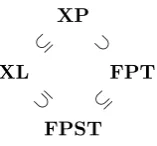
Summarizing our knowledge of the strongly uniform parameterized complex-ity classes we get the diagram in Figure 1. The diagram can be amalgamated with similar lattices for the uniform and nonuniform classes.
⊆ ⊂ ⊆ ⊆
FPST FPT XP
[image:19.595.258.337.125.198.2]XL
Figure 1: The containment order of selected classes of parameterized complexity.
for some constructible g, e. Of course, in the setting of time complexity ‘con-structible’ would be time constructible and in that of space complexity it would be space constructible.
The classical and open question L =? P has an immediate equivalent in the realm of parameterized complexity theory, namely whether nonuniformXL equals nonuniformXP. Indeed, if we haveL=P, then slices of a parameterized problem are inLif and only if they are inP, and vice versa. It is possible to drop the nonuniformity predicate, because given a P-algorithm we can effectively construct a reduction running in logarithmic space to the circuit value problem [3] and ifL=Pholds there exists anL-algorithm for the circuit value problem. Indeed, the concatenation of the reduction and the algorithm for the circuit value problem constitutes an effective transformation of arbitraryP-algorithms to L-algorithms, approving the omission of the nonuniformity predicate. In addition, looking closely at our transformation, we see that if L = P holds it is possible to bound the value of the constant coefficient of a logarithmic space complexity based on the exponent in the associated polynomial space complexity, showing thatFPST=? FPTtoo is equivalent toL=? P, as claimed by Flum and Grohe [18].
Cai, Chen, Downey and Fellows state that equality ofLandPis furthermore equivalent to equality of XL and FPT [9]. However, if this claim holds we would conclude that equality of LandPimplies equality of FPTandXP, but that is forbidden by Theorem 3. Thus they would have proven L 6=P. One shortcoming we note in their proof is the assumption thatFPTis closed under xl-reductions, a type of reduction we will deal with shortly. Such a property of FPTis yet to be proven.
Just as we have fpt-reductions and their relatives for the analysis of param-eterized time complexity, we have reductions for the analysis of paramparam-eterized space complexity too. Also, just as standard definitions of fpt-reduction had a shortcoming, standard definitions of reductions for parameterized space com-plexity [9, 15, 17] have one.
Definition 20. A language map from one parameterized problem to another, mapping (x, k) to (x0, k0), is an fpst-reduction if there are constants c, d, and computable, non-decreasing functionsg, h:N→N, such that we have:
1. each character of (x0, k0) is uniformly computable in spaceg(k) +clog|x|, independent of all other characters;
The shortcoming of standard definitions is once more in requirement 2 of the above reduction, of which the first part,|x0| ≤ |x|d, is usually unjustly omitted. Definition 20 generalizes to related reductions for all of our parameterized space complexity classes and each of these classes is minimal for its correspond-ing reduction, analogous to what we found in Lemma 6. The somewhat contrived space usage limit is an established [3] way to make these reductions actual re-ductions. With the more intuitive requirement of computability of (x0, k0) in its entirety in space g(k) +clog|x|, there might not be enough space to actually hold (x0, k0), and an equivalent of Theorem 5 would not be possible.
Theorem 10. The language maps that are fpst-reductions are reductions.
Proof. Like before, it suffices to prove only that the class of fpst-reductions is closed under composition. Let f1 and f2 be fpst-reductions of signatures that
admit the compositionf2◦f1. We will subscript all auxiliary symbols from the
definition according to the map they belong to.
1. We alter the procedure for computingf2so that each time a character of
(x0, k0) influences its computation, it is computed from (x, k) by means of
f1and an index in (x0, k0). By the time bound used in Theorem 9, (x0, k0) has a length in O(2g1(k)|x|c1) so the space needed to keep an index in
memory is no more thang1(k)+c1log|x|plus a constant. Up to a constant that is of no significance, this yields a procedure for computing f2◦f1
in space 2g1(k) + 2c1log|x|+g2(k0) +c2log|x0| ≤ 2g1(k) + 2c1log|x|+
g2(h1(k)) +d1c2log|x|. Hence each character off2◦f1 is computable in spaceg(k) +clog|x|withc= 2c1+d1c2 andg(k) = 2g1(k) +g2(h1(k)).
2. Identical to the corresponding part of the proof of Theorem 5.
A related characterization of tractability by kernelizations is possible in the case of fixed-parameter space tractability too.
Definition 21. A language map from one parameterized problem to another, mapping (x, k) to (x0, k0), is aspace kernelization if there is a constantc, and a computable, non-decreasing functionh:N→Nsuch that we have:
1. each character of (x0, k0) is uniformly computable in spaceclog|x|, inde-pendent of all other characters;
2. |x0| ≤h(k) andk0 ≤h(k) hold.
We call (x0, k0) thespace kernel of (x, k). A parameterized problemA isspace kernelizable if there exists a space kernelization fromAto itself.
A more practical version of the first requirement requires (x0, k0) to be
Algorithm 2 A space kernelization for VC. The input consists of a number of vertices, n, and an adjacency matrix, (Xi,j)0≤i<j<n, for a simple graph of
n vertices. All variables except X0, which is only written to, are restricted to usingO(logn) space. The degree of theith vertex in accordance with adjacency matrixX is written as deg(i: X). Conceptually, the algorithm is no different from Algorithm 1.
Input: An undirected adjacency matrixn,(Xi,j)0≤i<j<n and a parameterk
Output: A space kernel (n0,X0),k0 of (n, X), k
n0←0
k0←k // without loss of generality, we assume k≤n
for alli in{0,1, . . . , n−1}do // first, determinen0 andk0 if deg(i:X)> kthen
k0←k0−1
else if deg(i:X)>0 then n0←n0+ 1
end if end for
if n0 ≤2k0kthen // a cover of size k0 might be possible i0 ←0
j0←0
for alli in{0,1, . . . , n−1}do if 0<deg(i:X)< kthen
for allj in {i+ 1, i+ 2, . . . , n−1} do if 0<deg(j :X)< kthen
X0i0,j0 ←Xi,j //X0 is a write-only variable j0←j0+ 1
end if end for i0←i0+ 1 end if end for
else // construct a trivial rejecting space kernel n0←1
X00,0←true
k0←0 end if
before, space kernelizations are very real. An example is Algorithm 2, which shows that VCis space kernelizable.
Of course, space kernelizability interests us because it is related to space tractability.
Lemma 11. A parameterized problem is in FPSTif and only if it is decidable and space kernelizable.
Proof. The proof is the same as that of Lemma 4, except that instead of running
φ with a time bound of|x|c+1, we run φwith a space bound of (c+ 1) log|x|
and abort as soon as φ tries to use more space. If φ did not terminate, we have (c+ 1) log|x|< g(k) +clog|x|and consequently|x|<2g(k). The mapping
k7→2g(k)meets the requirements onhin definition 21 of being computable and non-decreasing.
Note that the bound on the size of the kernel that this proof provides is exponential in g, which is to be expected in light of the proof of Theorem 9. However, the bound is not very tight, as can be seen from our kernelization for
VC. Both Algorithm 1 and Algorithm 2 provide a kernel of sizeO(k4). Since
the unparameterized version of VCis complete forNPunder Karp reductions, it is unlikely that the size of a polynomial kernel [6] corresponds to the running time component gof anFPT-algorithm, as that would implyP=NP.
Like kernelizations in the case of time tractability, space kernelizations have a practical interpretation. Consider a data provider connected to a communi-cation channel [11], such as a computer storage device or a database server in a network, that provides structured data, say in the form of graphs. If we ask it a graph with the intention of checking whether it has a vertex cover of some size, the applicability of space kernelization becomes apparent. Without using space kernelization there is no guaranteed limit on the amount of data that needs to be transfered as a result of the query. If, however, we notify the provider of our intention and the provider implements space kernelization, it is sufficient for the provider to yield a space kernel, thus obtaining a guarantee on the amount of data to be transfered. The important observation is that this does not move the computational burden in terms of usage of space resources onto the data provider, because the space kernelization algorithm requires only a logarithmic amount of space and the space kernel can be communicated directly, without storing it on the side of the data provider. In general, this suggests that it is beneficial for data providers to implement a rich query language, enabling specification of intended data usage and its associated opportunities for em-ploying space kernelization. This pattern is of course already in use in many different forms. Computer storage devices are almost always addressable and many database query languages have high expressive power. Thus we can think of space kernelizations as a means of limiting data transfer and we have found a practical application of the analysis of fixed-parameter space tractability.
the notion of a parameterized problem being natural is not stable under loga-rithmic space reductions, thus the inclusion of VC inFPST does not directly give us the inclusion inFPSTof all natural parameterized versions of problems inNP. Additionally, Flum and Grohe [17] showed that completeness forFPST is not a very interesting property since trivial parameterizations of problems in Lare already complete forFPST. Luckily, though, there are also nontrivial pa-rameterizations that are natural, as we have withVC. In the limited research on parameterized space complexity, already quite a few parameterized problems of which the parameter is undoubtedly natural are classified [9, 15]. We will focus here on stretching the notion of parameterizations being natural, adding parameters until we can prove that a problem is inFPST.
The longest path problem is NP-complete and in FPT when given the obvious parameterization consisting of the desired path length [6]. A more generously parameterized version is the following.
Problem ((l, d)-Path). Longest path.
Instance: G, a directed graph.
Parameter: (l, d).
Criterion: Gdoes not contain a path of length land the maximum outdegree inGisd.
First, note that it is possible to verify whetherdis the maximum outdegree inGinO(log|G|) space. Next, any path of lengthlin a graphGwith maximum outdegreedcan be specified as a starting vertex plus a list of thel consecutive outbound edges. This specification takesO(log|G|+llogd) space. Conversely, in O(log|G|+llogd) space it is possible to enumerate all potential paths of lengthl in G. Verifying that no such potential path is present in the graph is the inverse of testing if any such potential path is present in the graph, which consists of the following checks.
1. All specified outbound edges are present inG.
2. The specification specifies an actual path, that is, it does not contain loops.
Given a specification of a path in O(llogd) space, the first check can be im-plemented by a simple graph traversal in O(log|G|) additional space, but the second is slightly more involved. A space efficient way of checking whether no loops are specified is by sequentially generating all pairs of vertices along the potential path and check whether no pair is made up of the same vertex twice. This too can be implemented inO(log|G|) additional space, hence we kept our space usage within O(log|G|+llogd) and have found an FPST-algorithm for (l, d)-Path.
In a similar fashion, we can find a parameterization of the connectivity prob-lem, which is complete for NL [3], with which the connectivity problem ends up inFPST.
Problem ((l, d)-STCon). Connectivity.
Instance: (G, s, t), whereGis a directed graph containing verticessandt.
Criterion: There is a path inGfromstotof length at mostland the maximum outdegree inGisd.
Arguably a more natural parameterization would be one that excludes the maximum outdegree,d. In that parameterization, the problem has been studied by Elberfeld, Stockhusen and Tantau [15]. Their investigation focussed on the amount of nondeterminism needed by a decision procedure as a function of the parameter and was part of studying a parameterized analogue of NL. Our pa-rameterized version, (l, d)-STCon, of the connectivity problem, however, needs no nondeterminism and is inFPST. Like before, all paths of length at mostl, starting atscan be specified inO(llogd) space. Checking that a potential path contains no loops is not necessary for this problem. The only checks that need to be performed are whether the potential path is present inGand whether it ends int. As these are possible in spaceO(log|G|), it follows that (l, d)-STCon is in FPST. Of course, this is comes as no surprise considering our result with (l, d)-Path, but we do feel the indication that the path length and outdegree play a substantial role in the space complexity of the connectivity problem is noteworthy.
The final problem we will discuss here is the circuit value problem, which is P-complete [3]. In light of the previous two problems, we think of a circuit as a labeled directed acyclic graph, and our parameterization looks as follows.
Problem ((h, d)-CV). Circuit value.
Instance: (C, x), whereC is a circuit andxa suitable input toC.
Parameter: (h, d).
Criterion: Coutputstrueonx, the height ofCishand the maximum fan-out inC isd.
We claim that (h, d)-CVis inFPST. Since the height of the circuit equals its maximum path length, it is possible to specify each path through the circuit inO(hlogd) space, much like we did with the previous two problems. Moreover, we can execute a depth-first traversal of the circuit in O(hlogd) space and retain partial outputs for all gates along a path within that space bound. Being able to keep track of partial outputs is crucial and hinges on the fact that the operations at the gates of the circuit are associative. Associativity allows us to merge the outputs of two inputs to a gate of arbitrary fan-in into a single partial output. Thus, partial outputs are of constant size and we see that indeed we can compute the output of a circuitCgiven inputxinO(log|C|+hlogd) space by doing a depth-first traversal. Hence, (h, d)-CVis in FPST.
There is a difference between the role of the parameterdin the first two prob-lems and in the last problem. In (l, d)-Pathand (l, d)-STConthe parameterd
can be substituted for an alternative parameterd0, the maximumindegreeinG.
However, replacing the parameterd in (h, d)-CVby a parameter d0 represent-ing the maximum fan-in in C, we run into trouble. In that case, the number of gates in the circuit can be upper bounded by a function of the parameters,
|C| ≤(d0)h, which, as we will see in Section 7, makes the problem trivially a
maximum fan-out. This reminds us of a result obtained by the probabilistic method [26], in particular as a consequence of Lov´sz local lemma, for the sat-isfiability problem [21, 27]. Namely, without clauses of a formula in conjunctive normal form sharing variables, the formula is satisfiable. Of course, on such for-mulas the satisfiability problem is easily decided. It appears that this is part of a more general result regarding the linkage between the outdegree in a directed acyclic graph and the complexity of problems defined on them.
6
Two-Part Codes
Descriptive complexity is involved in our study of parameterized complexity. Using some original definitions this involvement opens the door for structural parameterized complexity theory.
What makes a natural problem natural is best left a matter of aesthetics, but for parameterized problems Cai, Chen, Downey and Fellows hint at a property that would make a good requirement [9].
Definition 22. A parameterized problemAissmooth if, for the appropriaten
and allk1, k2∈Nn, we have:
k1≤k2 =⇒ Ak1 ⊆Ak2,
where the first inequality is taken componentwise. A smooth parameterized problemA is said to converge to the problem
A∞=
[
k∈Σ+
Ak.
The three problems of the previous section, (l, d)-Path, (l, d)-STCon and (h, d)-CV, as well as VC are all smooth. Informally, a parameterized prob-lem, A, being smooth suggests that its slices approximateA∞ from below. For
(l, d)-STConand (h, d)-CVthis is certainly true. Both exhibit convergence to their classical counterparts. For the other two parameterized problems, how-ever, the convergence would be to Σ+. Cai, Chen, Downey and Fellows name
parameterized problems of the former sortstandardized and observe that all pa-rameterized problems can be turned into standardized ones. This can be done by copying all or part of the parameter into the instance. For example, a stan-dardized version of (l, d)-Pathis the following.
Problem. Standardized longest path.
Instance: (G, l), whereGis a directed graph.
Parameter: (k, d).
Criterion: Gdoes not contain a path of length l, the maximum outdegree in
Gisdand we havel≤k.
The standardized problems that receive the most study are those for which fixed-parameter tractability results are known, whereas classical tractability re-sults for the problems they converge to are not. The parameter of such stan-dardized problems represents a source of complexity. However, there may be different fixed-parameter tractable standardized problems that converge to the same problem that is potentially intractable in the classical sense. For the ver-tex cover problem, Jansen and Bodlaender [24] have provided a parameterization different fromVCsuch that the parameterized problem is still kernelizable, thus fixed-parameter tractable. Question about the possibility of essentially different sources of complexity embodied by different fixed-parameter tractable standard-ized problems converging to the same potentially classically intractable problem are not prevalent in current fixed-parameter complexity research.
For all of our smooth parameterized problems there exists an upper bound to the parameter value with which an instance first occurs. These upper bounds only depend on the size of the instance. The existence of such upper bounds in practical applications of parameterized complexity theory is no surprise, because at some point the parameter dependent part of a complexity measure will start to dominate the part dependent on the instance size. Indeed, if this were not the case, the parameter had little to offer anyway.
The approximating characteristics of parameterized problems have been studied more formally in the context ofpolynomial time approximation schemes [14, 18]. Given an optimization problem, there is a strong connection between it having an efficient polynomial time approximation scheme and it being fixed-parameter tractable when fixed-parameterized by the potential value of optimal so-lutions.
Here, we will pursue a development of the informal notion of approximation by slices, independent of more classical approximation schemes. When provided a smooth parameterized problemAand anx∈Σ+ that is eventually in a slice
ofA, we interpret the parameter values with whichxis inAas capturing some upper bound on the resource complexity ofxinA. Certainly, bigger parameter values grant more of the resource at hand. This view motivates a complexity driven description of the instancexby means of a two-part code. The first part of the code specifies a slice and with it a complexity, the second part specifies an index within that slice.
Definition 23. We denote the index of some x ∈ Σ+ in a problem B by
rank(x : B) = k{y|y∈B ∧ y≤x}k, where the inequality is the inequality induced by the standard encoding ofNin Σ+. The parameter complexity of an instancexwith respect to a parameterized problemAis
pc(x:A) = min2|k|+|rank(x:Ak)|
(x, k)∈A . We take the minimum of the empty set to be∞.
The constant 2 in front of the specification of the slice is there to be able to tell the two parts of the code apart. If a parameterized problem converges to Σ+, the parameter complexity with respect to that problem is never∞.
of encoding instances, it relates to a compression method whenever the param-eterized problem is decidable. For example, in the case of VC, it tells us that we can encode a graph as the size of a vertex cover in the graph followed by an encoding that is only possible for graphs with a vertex cover of the given size. Immediately, we see that for smooth parameterized problems the slice se-lected by the parameter complexity will always be the first slice containing x. Based on this, we can boost the compression performance by not working with the smooth parameterized problem, but a cleaned up variant.
Definition 24. Thepurification of a smooth parameterized problemA is the problem
A℘={(x, k)|(x, k)∈A ∧ (x, k−1)∈/A}.
In the purification of a problem, instances only occur with their lowest pa-rameter value. An important fact about purifications is that if a smooth param-eterized problem is in one of our paramparam-eterized complexity classes, its purifica-tion is too. This is a consequence of the fact that our parameterized complexity classes are closed under finite applications of set-theoretic operations, including complementation.
Now, for VC, the encoding of an instance x associated with pc(x : VC℘) consists of the size of aminimum vertex cover followed by an encoding that is only possible for graphs with aminimumvertex cover of the given size. In situ-ations where vertex covers play a central role, this is a highly efficient encoding scheme. Note, though, that this encoding scheme internalizes all computational difficulty in the instances. Any smooth parameterized problem becomes com-putationally trivial when defined for inputs following the encoding associated with the problem. For example, given a graph encoded using the size of its min-imum vertex cover, it is trivial to determine if it contains a vertex cover of any given size.
There is a relationship between parameter complexity and Kolmogorov com-plexity, the latter of which we will indicate by Ct,s, wheretandsrepresent time and space bounds respectively [26].
Lemma 12. For every decidable parameterized problem A there exists a con-stant cand bounds t, ssuch that for all xwe have
Ct,s(x)≤pc(x:A) +c.
Proof. We may assume pc(x:A)<∞. Let (k, i) be an encoding ofxaccording to its parameter complexity with respect toA. That is,|(k, i)|= pc(x:A) and
xis the ith element of Ak. By decidability of A, it is possible to generate all
members ofAk in order. In particular, we can find the ith element of Ak. As
functions of (k, i), the time and space needed for this reconstruction ofxdepend solely on the time and space needed by a decision procedure forA.
The claim follows, with the additive constant c depending on the above procedure, which in turn depends onA.
Definition 25. A parameterized problem A is informative if there exists a functionf : Σ+→
Nsuch that for every parameterk∈Σ+ and constantc∈N we have
k(Ak∩Σ≤cf(k))k ≤ kΣ≤c(f(k)−1)k. (1)
More specifically, we then say that Aisf-informative.
Note that for an informative smooth parameterized problemA, the above limit is not required to hold for A∞. Relating to the works of Sipser, Li and
Vit´anyi [26] we note that a parameterized problem is informative if its slices are meager with a uniform rate of convergence. In any informative parameterized problem, the initial segments of each slice get increasingly empty as they grow in size. This should be thought of as instance sizes outgrowing parameter values. From this perspective, informative parameterized problems make sense because the additional resources provided by a parameter do not scale with the size of the instances and are thus only expected to aid decision for a limited subset of elements. In general, thinking about the distribution on the instance size that a parameter value induces may provide insight, even when a parameterized problem is not informative.
Since finite unions of meager problems are again meager, a parameterized problem is informative if and only if its purification is informative. This is po-tentially helpful in proving parameterized problems informative. Many param-eterized problems are informative and a proof can often be given via a combi-natorial argument. We will do so forVC.
Lemma 13. Under standard encodings of labeled graphs, VC, and thus VC℘
too, is informative.
Proof. For readability, we will not track all constants, additive or multiplicative, through this proof.
Standard, bijective, encoding by means of an adjacency matrix of labeled simple graphs withnvertices shows that there are 2O(n2)
different such graphs. We want to know how many of these graphs have a vertex cover of sizek. An upper bound on this number is provided by looking at an alternative encoding of graphs with n vertices and a vertex cover of size k. These graphs can be encoded by givingkvertices that make up a vertex cover followed by a reduced adjacency matrix of size k×n. A specification of all the edges in this way is possible by definition of a vertex cover. Thek vertices of the vertex cover can be specified within lengthklogn. Every graph ofnvertices with a vertex cover of size k thus admits a specification, although not uniquely, of lengthO(kn). Proving that (1) holds forVCis now possible by giving a functionf so that for all constants cthe number of graphs having a vertex cover of size kand a size
cf(k) specification under the standard encoding is less than 2c(f(k)−1). Ignoring some constants, we may thus setn=pcf(k) =√cpf(k) and by the alternative coding we get an upper bound to the number of graphs of 2k√cp
f(n). Focussing
on the exponents and moving the factors depending oncto one side, this leaves us to find a function f so that, regardless ofc, we have
kpf(n)≤√c(f(k)−1).
The functionf(k) =k2+ 2 behaves as desired and we may conclude that
VC
Informative parameterized problems provide a bridge between classical com-plexity theory and parameterized comcom-plexity theory. We have seen param-eterized problems that are in FPST and FPT, but converging to classical problems inNP. If every such parameterized problem is informative, the addi-tional resources granted by the parameter are apparently essential for slice-wise tractability and aid only a limited number of instances. In other words, there are instances of the classical problem requiring arbitrary additional resources, showing that the classical problem is indeed intractable. Of course, this line of reasoning asks for all parameterized problems in some class to be informative, which is a highly nontrivial question. The following general result is a conse-quence of Lemma 12, but we point out that the lemma requires the parameter-ized problem to be decidable, so the result is only usable for strongly uniform parameterized complexity classes.
Theorem 14. For any decidablef-informative parameterized problemA con-verging to Σ+, random strings make hard instances. Here, a hard instance
is an instance x that only occurs with parameter values k for which |x| is in
O(|k|f(k)).
Proof. Letxbe a string that cannot be compressed by more than a given con-stant. By Lemma 12, we get that this means that there is a constant r such that|x| −r≤pc(x:A) holds. Suppose thatxis inAk. We prove that|x|is in
O(|k|f(k)) with the hidden constant depending onr. By equation 1, the sec-ond part of the two-part code compresses strings of length cf(k) by at least c
characters. Since x cannot be compressed by more thanr characters and the first part of the two-part code has length 2|k|, the length ofxis upper bounded by (r+ 2|k|)f(k).
By the incompressibility theorem [22, 26] there are strings of any length that cannot be compressed by more than a given constant. Thus there are infinitely many hard instances for any informative parameterized problem.
It would be more attractive if we could define hardness of an instancexas
x only occurring with parameter values k for which |x| is in O(f(k)). This strengthening of Theorem 14 may well be possible, at least for a particular class of parameterized problems. A good candidate for such a class is the class of smooth parameterized problems. On these problems we can push the enve-lope of compression efficiency by looking at compressibility with respect to the purification of problems. Nevertheless, the definition used does a fair job cap-turing hardness. In algorithms, the dependency on the parameter is often of a big enough magnitude for the additional factor|k|to be irrelevant.
The restriction on the convergence of A to Σ+ in Theorem 14 could be loosened. Indeed, with minor modifications the same proof holds for parame-terized problems converging to any exponentially dense problem. As this is not the major value of the theorem, we valued clarity more than generality in this matter.