Reliability Modeling of Infrastructure Load-Sharing
Systems with Workload Adjustment
Qiuzhuang Sun, Zhi-Sheng Ye, Matthew Revie, and Lesley Walls
∗February 6, 2019
Abstract
Motivated by the need to support effective asset management of infrastructure systems, this paper presents a novel reliability model for a load-sharing system where the operator can adjust component work load to balance system degradation. The operator intervention effect, combined with other system complexities, makes modeling reliability interesting and challenging. We first develop cost modeling for a load-sharing system that has experienced operational service at the time of analysis. The system replacement process is modeled as a delayed renewal process for which the expected operational cost of the system is derived. A numerical algorithm is proposed to compute the cost, and the error bound is shown to be of order O(n−1). Next, we extend modeling to consider multiple heterogeneous
systems located at different sites within the infrastructure network. Heterogeneities here refer to possible cross-site differences in the operating environments and the operators’ actions. When the heterogeneities are observable, we model as covariates; otherwise, we model as random effects. Statistical inference methods are developed for the proposed models. An example using real data from a water utility illustrates the logical model behavior given parameter choices as well as showing how analysis might inform asset management.
Keywords: Delayed renewal process, degradation failure, cumulative work load, Gamma pro-cess, load-sharing system.
Acronyms
RGF Rapid gravity filter CWL Cumulative work load RS Riemann-Stieltjes SF Survival function
∗This work is supported in part by Natural Science Foundation of Jiangsu Province under grant
PDF Probability density function CDF Cumulative distribution function IG Inverse Gaussian
MLE Maximum likelihood estimator
Notations
T Time to degradation failure of the system
Xi CWL-to-degradation failure of component i S CWL-to-degradation failure of the system
U(t) CWL to the system at t
N Number of components in a system
z Time that system has been in operational service at t= 0
u CWL at t = 0
y Annual average turbidity
C(τ) Expected cost over mission time τ µ Mean of the IG distribution for Xi
λ Shape parameter of the IG distribution for Xi γ Scale parameter of accumulation of the CWL
process
v Shape parameter of accumulation of the CWL process
CO Operational cost of a system component Cr Replacement cost of a system component Cs Fixed system replacement cost
1
Introduction
An infrastructure system, such as a wind farm, water treatment works or power sta-tion, can consist of multiple functionally-identical components that synergistically work together and share the total load to the system. In order to achieve reliable system functioning, components are designed to be highly reliable in the sense that they sel-dom suffer from sudden failures. Nevertheless, components might degrade gradually with usage. Degradation in the condition or performance of a component can be measured using sensors, e.g., vibration frequency of a machine [1], wear particles in the lubrication oil [2], and the erosion level of an induction furnace [3]. Without accurate measurement, degradation can also be perceived visually, e.g., pitting corrosion on a turbine blade and clustering of the sand in rapid gravity filters of a water filtration process. A component is replaced when the degradation level is deemed unacceptable, which is commonly known as a degradation failure [4, 5]. A review on degradation analysis can be found in [6].
components. Using this work load adjustment strategy implies that the degradation levels of all components are managed and maintained at a similar level. Specifically, we have observed this degradation management strategy for rapid gravity filters (RGFs) which are used during the water filtration process in water treatment works. For RGFs, as well as other critical components, the water utility have adopted this approach for several reasons. First, the fixed replacement cost is high relative to the variable cost. Therefore, by managing the degradation of all RGFs used within a water filtration process, the performance of these components can be kept approximately at the same level, and they can be replaced collectively when the performance is deemed unsatisfactory. Second, all RGFs are required to be working in order to handle the peak demand. Many water treatment works have multiple RGFs, and the failure of one or more components within the system impacts the ability to handle the peak demand. The loss of this service level is regarded as a system failure.
In this study, we propose the work load adjustment strategy discussed above and exemplified in the context of a water filtration process. The work load adjustment strat-egy can be generalized to a wider class of infrastructure systems which involves human operators with the ability to make process interventions. Such systems can be regarded as load-sharing systems, since the components share the total work load of the system according to a defined set of sharing rules [7–10]. Reliability modeling of a load-sharing system with managed component degradation is challenging because components in the system are used intermittently.
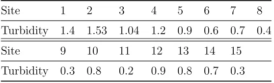
Previously, Ye et al. [11] proposed a framework to model reliability based on the con-cept of cumulative work load (CWL). As shown in Fig. 1, the framework consists of three steps. The first step focuses on the CWLs-to-failure, initially at component level then the aggregation of component CWL-to-failure to obtain the system CWL-to-failure. The second step obtains the CWL process for the system. The last step combines the system CWL-to-failure distribution and the CWL process to reach the time-to-failure of the system. The merits of this framework are as follows. First, components are used in-termittently and thus it is not appropriate to use the chronological time scale. The CWL reflects the component usage, which affects the degree of component degradation. Second, data can be more routinely recorded for the CWL process to the system and the compo-nent CWLs-to-failure, meaning that data are likely to be available to populate the model. Third, the model allows us to obtain the system CWL-to-failure from data captured for the component CWLs-to-failure. For example, when a system comprising multiple com-ponents is replaced because the managed degradation levels of all comcom-ponents are beyond an acceptable threshold, then we have multiple component CWLs-to-failure. Statistical inference based on the component CWLs-to-failure will be more accurate given the data. Even if empirical records are not available, then subject matter expertise can be elicited from, say, relevant operators who can reason through the probabilistic uncertainties in the CWL-to-failure based on their greater understanding and experience of component, rather than system, failures [12].
Component CWL-to-failure distribution
Sum up to get system CWL-to-failure distribution
Obtain the CWL process
[image:4.595.156.441.69.201.2]System time-to-degradation-failure distribution
Figure 1: A framework for a load-sharing system with managed component degradation proposed in [11].
the management of assets of varying experience and degrees of degradation. For exam-ple, a water utility may have RGFs with different operational experience between water treatment works. Second, the model does not have the capability to represent situations where there are multiple systems, each with one or more components that are operated simultaneously, and a centralized maintenance resource allocation process. For example, consider the geographical dispersion of the sites of water treatment works, i.e. the sys-tem, for which we want to model the RGFs as key components. The heterogeneity in site location implies variation in environmental factors which can impact, for example, input water quality and volume. Asset managers tend to believe that for the same volume of water processed, sites which process water with higher levels of impurity will degrade faster. Additionally, each water treatment works will typically have its own operators. The experience and skill of the operators can also vary and so it is reasonable to assume that sites processing the same volume of water with identical levels of impurity may degrade at different rates due to operator effects.
In view of these two deficiencies, this study extends the model of [11] in two distinct ways. First, we develop a cost prediction model for an in-service system. Second, we develop a model to capture the differences in the degradation of components across mul-tiple systems. A random effect model is developed to incorporate the impact of influential factors that contribute to the rate of degradation. For both model developments, statis-tical inference of the necessary parameters are discussed. The first model development provides expected cost predictions which can aid understanding of future failure profiles and hence resource implications for asset management. The second model development extends the analytical capability to account for the effects of influencing factors so that more meaningful comparisons can be made between systems which are competing for resource.
The contribution of this paper is twofold. Scientifically, the development of the model-ing methodology makes a distinctive contribution to the existmodel-ing literature on reliability models for load-sharing systems. More practically, the models are aligned with asset management having been motivated by and illustrated using industry data from a water utility. Indeed in reality, this research has been conducted to support analytical special-ists within the water utility by providing more advanced modeling methods, from which decision support tools for asset managers can be created.
mod-els the impact of influencing factors in changing the component CWL-to-failure. Section 5 presents inference methods for both a single system and multiple systems. Section 6 illustrates the logical behavior of the model as well as showing the principles of analysis to aid asset managers. Section 7 concludes and shares suggested further work.
2
Model Setting for a Single System
Consider a system with N functionally-identical components. Assume that the compo-nents are subject to degradation failures only. Our model is based on the concept of CWL. The motivation for using the CWL concept is that the cumulative usage of a com-ponent induces its degradation and CWL can be observable in practical contexts. We assume the failure rate of a component increases in its CWL, and the CWL-to-failure is different for each component. Hence we model the CWL-to-failure as a random variable. While CWL can be considered a measure of cumulative exposure as used in, for exam-ple, [13] who described the effect of a dynamic covariate on the failure time distribution, our study models the cumulative work load as a stochastic process, which is based on a physical interpretation of degradation of a system of components. Interested readers may refer to [11] for a detailed illustration of the CWL-to-degradation-failure framework. In general, the following assumptions are used for a single system.
• The CWL to the system is a monotone increasing stochastic process U(t);t ≥ 0, which has stationary increments. That is, fort, s >0, U(t+s)−U(s) is independent of U(s), has positive support, and has the same distribution as U(t). Here t = 0 stands for the date of analysis (say, today), which is different from the installation date of the system.
• During system operation, the operator dynamically allocates the work load to the components based on the work load magnitude and the component degradation levels. Through the work load adjustment, the degradation levels of all components are managed so that the time to degradation failure of each component does not differ too much from each other.
• The component CWL-to-degradation-failuresXi,i= 1, . . . , N, are independent and
identically distributed (i.i.d.) and follow an inverse Gaussian (IG) distribution, i.e.,
Xi ∼ IG(µ, λ), µ, λ ≥0, with probability density function (PDF) and cumulative
distribution function (CDF) as
fIG(x;µ, λ) =
λ
2πx3 12
exp
−λ(x−µ)
2
2µ2x
,
and
FIG(x;µ, λ) = Φ r
λ x
x
µ−1
!
+ exp
2λ µ
·Φ −
r λ x
x
µ + 1
!
,
for x >0, where Φ(·) is the standard normal CDF.
machines [14], the railway tracks [15], and the print head of color printers [16], to name a few. In the industry problem we consider in Section 6, the component subject to failure is the RGFs in a water utility. RGFs are used to filter impurities from raw water. The wear of RGFs occurs during the usage and, as a result, assuming that components are mainly subject to degradation-induced failures is reasonable. Further, we assume a com-ponent fails when its cumulative work load exceeds a random threshold and propose that this framework may be more flexible to characterize the failure behavior compared with the models traditionally reported in the literature, where the component fails when its observable degradation level exceeds a fixed failure threshold. Following [11], we assume the IG distribution can provide a reasonable model for the CWL-to-degradation-failure. Based on the CWL framework, the system fails when the system CWL U(t) exceeds the random thresholdS ≡PN
i=1Xi, which can be readily shown to follow an IG
distribu-tion S∼ IG(N µ, N2λ) [11]. This random variableS is the system
CWL-to-degradation-failure. On the other side, we can use Gamma process, IG process or compound Poisson process to model the system CWL process U(t). If the variation of the CWL process is small, we may use a linear function to approximate the CWL process. As an example, if the CWL process follows a Gamma process with scale parameter γ and shape parameter
v, then the PDF of the system CWL at time t is given by
gU(t)(u;vt, γ) =
uvt−1
Γ(vt)γvt exp
−u
γ
, u >0. (1)
3
Cost Analysis of an In-Service System
For an in-service system, we treat the replacement process as a delayed renewal process. This section derives the expected cost for such a system that has been operational for a period of time at t= 0. An algorithm is proposed to compute the renewal function. The rate of convergence of the numerical error is shown to be O(n−1).
3.1
The replacement process – a delayed renewal process
At time t = 0, the (N-component) system of interest may have been in operation for a period of time. For this system, the replacement process constitutes a delayed renewal process {Y, T1, T2,· · · } with the i.i.d. inter-replacement times Ti, i = 1,2,· · ·, and the
first replacement time Y following a different distribution. Here, Y can be regarded as the remaining useful life of the system. The distribution of Y depends on how long the system has been in use and how much work load it has processed. If we only know that the system has been in operation for z units of time at t = 0, the distribution of Y is given by
FY(t) = Pr(T > t+z|T > z) =
FT(t+z)−FT(z)
1−FT(z) .
If in addition to the operation time z, the CWL of the system at time t= 0 is available, then we can have a more accurate estimation for Y because the lifetime of the system is determined by its usage. Denote the CWL at t= 0 as u and thus the CWL at time t is
U(t) +u. Given u at time 0, the distribution of Y can be computed as
FY(t) = Pr(S < U(t) +u|S > u) =
Pr(u < S < U(t) +u)
The numerator can be expressed as Pr(u < S < U(t)+u) = Pr(S < U(t)+u)−Pr(S < u), where Pr(S < u) is simply the CDF of the IG random variable IG(N µ, N2λ), while
Pr(S < U(t) +u) can be evaluated as
Pr(S < U(t) +u) =
Z ∞
0
FS(v+u)gU(t)(v)dv. (2)
3.2
Expected cost over a finite time horizon
Based on the above assumption, the replacement consists of a delayed renewal process
{Y, T1, T2,· · · }, where the system starts anew after each replacement. Let N(t) be the
number of system replacements at time t, and m∗(t) = E[N(t)] is the renewal function
for the delayed renewal process. Suppose that the unit time operation cost of an N -component system isN CO, depending on the number of components. When the system is
replaced because of unsatisfactory performance, the replacement cost includes the price of each component, denoted byCr, and a fixed system replacement cost, denoted byCs. All
the components are replaced at the same time for the two reasons as discussed in Section 1. The simultaneous replacement can be achieved through the work load adjustment by operators. In our case study in Section 6, the RGFs degrade/wear gradually with usage. The degradation level of the filtering media cannot be measured precisely. Nevertheless, an operator can assess the degradation level by directly observing the filtering media. For example, dark spots and darkening of the media on visual inspection indicate that the RGF is aging. The measurements of output water quality from the RGFs can also help to assess the degradation level. Operators then select which RGF(s) to use based on their observation of the RGF degradation levels. Under this strategy, the degradation levels of all RGFs are balanced, so that all RGFs in a system fail approximately at the same time. The replacement time is assumed negligible compared with the time-to-degradation-failure of the system. The expected cost of an existing system operating within a predetermined time horizon τ can be expressed as
C(τ) =N τ CO+ (N Cr+Cs)m∗(τ). (3)
The expected cost (3) involves the delayed renewal function, which has to be evaluated numerically. Here we develop a numerical procedure to compute the delayed renewal func-tion. The procedure is based on the Riemann-Stieltjes (RS) sums method by partitioning [0, τ] into n sub-intervals.
We now consider the following delayed renewal process {Y, Z1, Z2, . . . , Zn, . . .} where Y has a survival function (SF) ¯F∗(t) and Z
n, n ≥1 have a SF ¯F(t). Conditional on the
first arrival, m∗(t) can be expressed as
m∗(t) =F∗(t) +
Z t
0
F∗(t−x)dm(x), (4)
where m(t) is the renewal function for the renewal process {Z1, Z2, . . . , Zn, . . .} with
renewal equation
m(t) = F(t) +
Z t
0
F(t−x)dm(x). (5)
Then m(tj),1 ≤ j ≤ n, can be numerically calculated iteratively. Its expression was
derived by [17] and is given by
˜
m(tj) =
F(tj) +Gj −F(tj−tj−1/2) ˜m(tj−1)
1−F(tj −tj−1/2)
, (6)
where ˜m(t0) = 0, tj−1/2 = (tj−1 +tj)/2 and Gj =Pj−1k=1F(tj−tk−1/2)[ ˜m(tk)−m˜(tk−1)].
We use ˜m(ti) to indicate that it is a numerical approximation of m(ti). Once ˜m(t1),
˜
m(t2),. . ., ˜m(tj) are calculated, we can approximate m∗(tj),1 ≤j ≤ n based on the RS
sums method, which is given by
˜
m∗(tj) =F∗(tj) + j X
k=1
F∗(tj −tk−1/2)[ ˜m(tk)−m˜(tk−1)].
According to our numerical experience, the above numerical method form∗(t
n) is very
accurate. The following theorem shows that the approximation error of the numerical procedure is O(n−1). The proof is given in the appendix.
Theorem 1. SupposeF(·) is twice differentiable in the interval[0, τ] with first derivative
f and bounded second derivative, and m(·) and F∗(·) are differentiable in [0, τ] with
bounded derivatives. If max{ti−ti−1;i= 1,2,· · · , n}=O(n−1), then m∗(tn)−m˜∗(tn) =
O(n−1).
4
Heterogeneities of Multiple Systems
In situations where multiple systems of the same type exist, there can be system-to-system differences in their degradation profiles. For example, a water utility has multiple water treatment sites and the raw water quality in one water treatment site may be significantly different from another site in a different location. Given the same functional performance of the filtering media, the CWL process depends on the quality of the raw water. It is expected that the more impurities in the raw water, the faster the degradation rate of the media and thus the shorter the CWL until failure. This implies that the quality of raw water affects the CWL-to-failure of a filter. Other possible causes of the heterogeneities include operators and environments. They are called influential factors in our study.
If information about the influential factors is available, then we can treat them as a covariate and incorporate into the component CWL-to-failure distribution. We assume that the influential factor is constant at a site. For example, data is available on incoming raw water quality to each water treatment site, hence we can model this factor as a constantyin a site, where a higher ymeans a better quality of the raw water, i.e., slower degradation of the RGF. Recall that the component CWL-to-failure X ∼ IG(µ, λ). The convention to model covariates is to let some parameters in the distribution of X be an increasing function of y. A largery leads to a larger CWL-to-failure X in general, while
E[X] =µ. Therefore, we can assumeµto be a function ofy. Some common choices for the link function between yand µare the power law, the Arrhenius law and the exponential law [18, 19]. An appropriate link function can be determined based on expert knowledge, or from data analysis. Suppose that we have chosen the power law, i.e., µ=ayb, where a, b >0 are parameters. Then the system CWL-to-failure S ∼ IG(N ayb, N2λ).
unobserved factor that affects the CWL-to-failure of a filter. Unobserved factors affecting the CWL-to-failure of a RGF include the skills of operators and local site environments. For example, high operator skill affects key process steps such as the quality of the back-wash, which is a regular procedure to cleanse the media. If the media is less clean, then the RGF needs to work harder and therefore degrades faster. Systematic difference in the CWL process between water treatment sites can occur because different locations serve areas with different population size and thus different demand rates. Local environments, e.g., humidity and temperature, also affect the demand rate and the CWL process.
The unobservable factors in the CWL process and the CWL-to-failure of the compo-nents (e.g., the RGFs) can be captured by random effects. Essentially, the random effects are unobserved covariates which vary over sites. The random effect in each unit is fixed yet unknown (e.g., the impurities of the raw water), and different units have different realizations of the random effects [20–24]. A special case of random effects is the frailty, which assumes the unobserved covariates have a multiplicative effect on the baseline fail-ure rate [25, 26]. For a comprehensive overview of frailty models, see, for example, [27]. In the following, we discuss how to use random effect model to capture these unobserved factors.
First of all, we discuss incorporation of random effects in the lifetime distribution for the component CWL-to-failure. For a system, we have assumed that the component CWL-to-failure X ∼ IG(µ, λ) while the system CWL-to-failure S ∼ IG(N µ, N2λ). The
environmental factors, (e.g., the raw water impurity) influence the means of X and S. Therefore, we can assume that µ is fixed and unknown for each site, and is random across all sites. The distribution of µcan be obtained from data analysis, as discussed in Section 5, or from expert knowledge [28]. One convenient method is to use the conjugate prior, which assumes 1/µ ∼ N(υ, σ2). To derive the component CDF of the system
CWL-to-failure in this case, we need the following lemma.
Lemma 1. SupposeZ ∼ N(υ, σ2). Then we have
E[Φ(aZ+b)] = Φ
aυ+b
√
1 +a2σ2
(7)
and
E[ecZ+dΦ(aZ+b)] = exp
cυ+d+ 1 2c
2σ2
×Φ
aυ+b+acσ2
√
1 +a2σ2
, (8)
where a, b, c and d are arbitrary constants.
The proof of Lemma 1 is given in the appendix. With the lemma, we can obtain the component CDF of the system CWL-to-failure as
FX(x) = Φ
υx−1
p
x/λ+λσ2 !
+ exp 2λ+ 2λ2σ2
Φ −(υ+ 2λσ
2)x−1 p
x/λ+λσ2 !
. (9)
The detailed procedure to derive Equation (9) is also given in the appendix. It should be noted that conditional on the random effects µ, the CWLs-to-failure of components in the same system are independent. However, they are dependent unconditionally. The CDF of system CWL-to-failure can be computed by integrating µ out of IG(N µ, N2λ),
which yields
FS(s) = Φ
υx−N
p
x/λ+N2λσ2 !
+ exp 2N2λ+ 2N2λ2σ2
Φ −(υ+ 2N λσ
2)x−N p
x/λ+N2λσ2 !
Next, we explain how we might capture random effects on the work load accumulation process for the cases of the Gamma process. We may assume that the CWL to system follows the Gamma process U(t)∼ gamma(vt, γ) with the PDF given in (1). Note that the mean of U(t) is γvt. We have argued that different sites will have different demand rate and so different accumulation rates for the CWL. Therefore, we may assume thatγ is different across sites. A tractable model results when γ−1 follows a Gamma distribution
with γ−1 ∼ gamma(κ, φ−1). Integrating γ out of Equation (1) yields the unconditional
distribution of U(t) as
gU(t)(u) =
φκΓ(vt+κ)uvt−1
Γ(κ)Γ(vt)(φ+u)vt+κ.
5
Statistical Inference
5.1
Single system
First we return to the scenario where we consider only one system (e.g., a water treat-ment site) which implies the random-effects model is not necessary. Under this scenario, we need to estimate the to-failure distribution and the CWL process. The CWL-to-failure distribution can be estimated using the usage data of each component upon replacement. Such usage data are available, e.g., from a meter embedded in the compo-nent. Let {x1, x2,· · ·, xN} be the CWL-to failure of N components, e.g., from several
replacements. Inference for the IG distribution has been well-addressed in the literature, e.g., Section 11.4 in [29]. We briefly recapitulate the procedure here. The log-likelihood function, up to a constant, is
l(µ, λ) = 1
2Nlnλ−
N X
i=1
λ(xi−µ)2
2µ2x i
. (10)
Maximizing this function yields the maximum likelihood estimators (MLEs) of µ and λ
as ˆµ= ¯x, the average of xi, and ˆλ=N/PNi=1(x−1i −x¯−1).
To estimate the CWL process, suppose we collect the CWL periodically, say, every day or every week. Let U = {u1, u2,· · · , uK} be the consecutive CWL measurements
from period 1 to period K and ∆u = {∆u1,∆u2,· · ·,∆uK} be the increments, i.e.,
∆ui =ui−ui−1 with u0 = 0 for convenience. Because we have assumed that the process
has stationary increments and the data collection interval is constant, the increments ∆ui should be i.i.d. samples. If we assume the CWL accumulation is a Gamma process,
then we can use a Gamma distribution to fit ∆u. Let ∆t be the collection time interval. Then the increments follow Gamma(v∆t, γ) and thus the log-likelihood function, up to a constant, is given by
l(v, γ) =K[v∆tlnγ−ln Γ(v∆t)] +v∆t K X
i=1
ln ∆ui−γ K X
i=1
∆ui.
The MLE can be obtained by first solving ln(v∆t/u¯) + lnu =ψ(v∆t) for ˆv, where ψ(·) is the digamma function, and ¯u and lnu are averages ofui and lnui, respectively. Then
ˆ
5.2
Multiple systems
Now consider the situation where we model multiple sites. If the raw water quality for each site is available then we can treat this factorz as a covariate and assume thatµis a function ofy. Suppose that we choose to use the power law relationµ=ayb, and that data
onM sites are available. For the ith site, the CWL-to-failure data are{xi1, xi2,· · · , xiNi}
and the raw water quality level is yi; and suppose the CWL process is observed at time
epochs {ti1, ti2,· · · , tiKi} with the associated CWL ui = {ui1, ui2,· · · , uiKi}. Then the
log-likelihood function is a slight modification of (10):
l(µ, λ) =
M X
i=1 "
1
2Nilnλ−
Ni X
j=1
λ(xij −aybi)2
2(a2y2b i )xij
#
. (11)
If the raw water quality is not observed, we use the random-effects models to capture the differences in the component CWL-to-failure distribution between different sites. De-note ωi1 = PN
i
j=1xij, ωi2 = PN i
j=1x−1ij and ωi3 = PN i
j=1lnxij. We then use the following
lemma to derive the log-likelihood function.
Lemma 2. Let Z ∼ N(υ, σ2). Then we have
E
exp
−1
2(aZ
2+ 2bZ+c)
=
(
(1 +aσ2)−1 2 exp
h
−2bυ+aυ2−b2σ2
2(1+aσ2) −
1 2c
i
, a >−σ−2;
∞, a <−σ−2.
Proof of the lemma is straightforward and thus it is omitted here. The log-likelihood function, up to a constant, can be then expressed as
l(λ, υ, σ2) = 1 2
M X
i=1
Nilnλ−ln(1 +λσ2ωi1)
− λωi1υ
2−2N
iλυ−Ni2λ2σ2
1 +λωi1σ2 −
(λωi2+ 3ωi3)
. (12)
Detailed derivation of (12) is given in the appendix. Direct maximization of this function yields the MLEs of the three parameters.
We now discuss statistical inference of the CWL process given that there are random-effects between different sites. Since we assume that the system CWL process follows the Gamma process with random effect, the likelihood function is given by
l(v, κ, φ) =
M X
i=1
κlnφ+ ln Γ(vtiNi+κ) (13)
−ln Γ(κ)−(vtNi +κ) ln(φ+uiNi)
+ M X i=1 Ni X j=1
v∆tijln ∆uij −ln Γ(v∆tij).
6
Example to Examine Model Behavior and Use
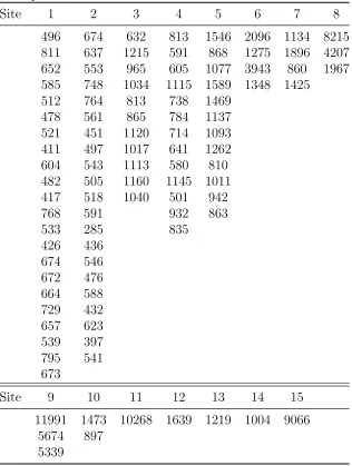
We use de-sensitized real data from selected water treatment sites owned by a water utility to illustrate the application of our proposed models. Tables 1 - 3 in the appendix provide the data for the CWL-to-failure of RGFs at fifteen water treatment sites, together with the typical CWL per annum and the average water turbidity at each of the sites. Turbidity is a measure of water quality and one intent of filtering is to reduce turbidity. While turbidity will naturally vary throughout the year for each site, we have taken a yearly average which is requisite for our example purpose since this average provides an indicative level of the typical raw water impurity. Using monthly demand from each site over an annual period, data which is recorded by the water utility although not shown, we can estimate the CWL process. The raw water quality can then be treated as a covariate. Note also that each site contains a different number of RGFs and, although not shown, it is known that each site is of a different size, has different operators, has different work load profiles and has filters of different ages.
Currently, the water utility forecasts the operation costs of their water treatment sites within a 5-year time horizon, so that they can assess the variation of maintenance and replacement spending from year to year for the multiple treatment sites. Motivated by this, we propose a cost prediction model with the consideration of the system hetero-geneity and the system current usage condition. Section 6.1 explains how we estimate model parameters from the data. Section 6.2 uses these estimates to compute the failure time distribution, the expected failure number, and the expected operational cost for a single system, and discusses the results for site 1 with the main purpose of sense-checking the model behavior. Section 6.3 then predicts the operational costs for multiple sites and discusses how the findings allow us to anticipate when the peaks in the cost spending may occur across sub-sets of the sites, and to illustrate how asset managers might gain insight into anticipated cost and failure profiles. Section 6.4 presents some sensitivity analysis and discusses the implications for our understanding of the model and its results.
6.1
Estimation of model parameters
We use an IG distribution with mean parameter µ= ayb and shape λ for the
CWL-to-failure of the RGF components, where yis the turbidity for the site. Based on the data, the estimates ofa, bandλare ˆa = 991,ˆb =−1.50 and ˆλ= 14285. These estimates are ob-tained by numerically maximizing the log-likelihood function (11), which can be achieved by most optimization functions in modern software, e.g., fminsearch in MATLAB.
We then use the monthly demand data to estimate the CWL process by assuming a Gamma process with random effects. By setting the time unit as one month, the estimates of parameters φ, κ and v are ˆφ = 98.15, ˆκ = 3.138 and ˆv = 1.038 through numerically maximizing the log-likelihood function (13). Let tmax= 12 and Ui(tmax) be the CWL of
the ith system at the end of the year. Then γi−1 for the ith system follows a Gamma distribution with shape parameter ˆvtmax+ ˆκ and scale parameter (Ui(tmax) + ˆφ)−1. We
can compute the estimates of γ for the 15 sites as
ˆ
γ = [118,63.0,119,24.3,36.2,37.0,30.4,59.4,39.5,37.8,35.9,17.5,23.8,21.8,21.7].
Time in year
0 5 10 15
Failure probability
0 0.1 0.2 0.3 0.4 0.5 0.6 0.7 0.8 0.9 1
New system
z=1
z=2
z=5
(a) CDF
Time in year
0 5 10 15 20 25
Renewal function
0 0.5 1 1.5 2 2.5 3
New system
z=1 z=2 z=5
(b) Renewal function
Time in year
0 5 10 15 20 25
Expected cost
0 20 40 60 80 100 120
New system
z=1 z=2 z=5
[image:13.595.88.497.79.508.2](c) Expected cost
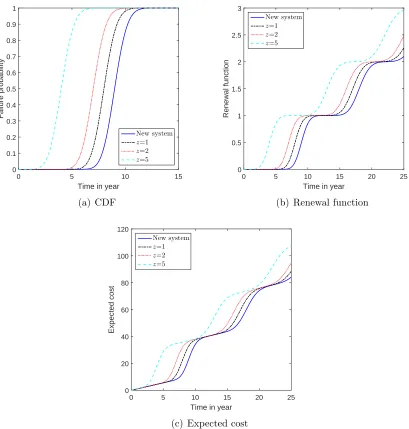
Figure 2: The CDF, renewal function and expected cost for Site 1 with specified years of past operation only.
cost is Cs= 5. The units used for the time, monetary values and the CWL are in years,
thousands of pounds and trillion of litres, respectively.
6.2
Failure behavior for a single site
Consider site 1 to illustrate the behavior of the model. For site 1, the average turbidity value is y = 1.4. From this, ˆµ = ˆayˆb = 598.2. First, let us consider the situation where
expected number of failure during a time horizon, the renewal function at the first five years should be near zero, as shown in Fig. 2(b). Similarly, the renewal function at time 10 (year) should be approximately equal one since there is a very high probability that the system has failed before this time. The system is replaced with a new one after failure, so there should be no failures at the first five years after the replacement. This explains why the renewal function keeps nearly constant from 10 to 15 (year). From Equation (3), the expected cost C(τ) is a function of the renewal function m∗(τ). When m∗(τ) keeps
nearly constant, the increase of C(τ) is mainly due to the operational cost. Because the operational cost is much smaller than the replacement cost for a system, the increase of
C(τ) is relatively slow during [10,15] and [20,25] (year) for the new site, as shown in Fig. 2(c). We can also see that the CDF shifts to the left as z increases as expected, since older systems with longer operational experience will have accrued greater degradation.
6.3
Analysis using the model for multiple sites
Now consider how the model can be developed for analytical support. Typically, there are constrained budgets for portfolios of multiple assets. The proposed model can aid managers to anticipate when peaks in spending might occur by providing insight about the failure profiles of individual assets and the associated maintenance costs.
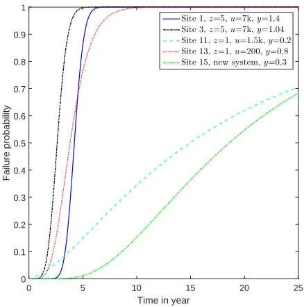
Using the same data and model as the previous section, Fig. 3 shows the degradation failure profiles for the RGFs at the sites of five water treatment works over a 25-year horizon. The sites vary in terms of number of RGFs as well as the age (z) and CWL (u) at the time of analysis, t = 0. The predictions show that sites 1 and 3 are almost certain to fail within the next 5 years, while the failure profiles of sites 11 and 15, in particular, are shifted to the right with only a 0.5 chance of failing in around 15 and 19 years respectively. The two sites whose CDFs indicate a higher median time to failure and greater variation are smaller in terms of the number of RGFs installed, younger in terms of calendar age as well as CWL, and have low turbidity in comparison with the three sites whose CDFs indicate failures are more likely to occur within a relatively shorter time scale. Sites 1 and 3 are very similar in all respects except the number of RGFs. Site 3, which has half the number of RGFs but a similar high average turbidity level as site 1, has the most left failure profile. For site 3, there is a 0.5 chance of failure in about 2.5 years from the time of analysis compared with 4.5 years for site 1. Site 13 has fewer RGFs but a mid-level average turbidity suggestive of a relatively high work load, and the model predicts a 0.5 chance of failure within around 4 years. While this prediction indicates failure may be earlier than for the largest site 1, there is greater variation in the CDFs for site 13 compared with sites 1 and 3. For example, there is a 0.9 chance that site 13 will fail in about 6 years but that site 1 will fail within 5 years.
Time in year
0 5 10 15 20 25
Failure probability
0 0.1 0.2 0.3 0.4 0.5 0.6 0.7 0.8 0.9 1
Site 1,z=5,u=7k,y=1.4 Site 3,z=5,u=7k,y=1.04
Site 11,z=1,u=1.5k,y=0.2
Site 13,z=1,u=200,y=0.8
[image:15.595.184.403.85.306.2]Site 15, new system,y=0.3
Figure 3: CDF for selected sites over a 25-year planning horizon.
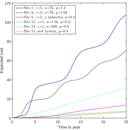
site RGFs, is more damped. The expected cost profiles of sites 11, 13 and 15 are lower as might be anticipated given their CDF profiles and the single RGF. Site 8 with three RGFs and two years of past operation has a cost profile higher than those for sites 11, 13 and 15, but it is still relatively much lower than the costs predicted for sites 1 and 3. Fig. 4 shows that it is expected £30m and £19m will be the costs associated with the failure and replacement of sites 1 and 3, respectively. Given a specified planning horizon, the asset manager can accumulate expected costs across sites within his portfolio.
Time in year
0 5 10 15 20 25
Expected cost
0 20 40 60 80 100 120
Site 1,z=5,u=7k,y=1.4 Site 3,z=5,u=7k,y=1.04
Site 8,z=2,uunknown,y=0.4
Site 11,z=1,u=1.5k,y=0.2
Site 13,z=1,u=200,y=0.8
[image:16.595.184.402.85.306.2]Site 15, new system,y=0.3
Figure 4: Expected cost for selected sites over a 25-year planning horizon.
allows an initial exploration of site specific effects to make an initial assessment of the likely impact of changing work load through, for example, changes to the operational processes.
Our analysis shows that the dynamic work load adjustment strategy leads to the variation of the expected annual cost for each site, e.g., see Fig. 4. Since each site has its own degradation behavior, the failure time distribution differs among the treatment sites. As a result, different sites may have different peak years for maintenance and replacement spending. As intended, the proposed model can predict the total cost for each site within a given time horizon and provide asset managers with insight when peaks in the operational cost may occur for each site.
6.4
Sensitivity analysis
To examine the sensitivity of C(τ) within the time horizon τ ∈ [0,25], we fix the re-placement cost, i.e., set Cr = 1 and Cs= 5 as above, but we change the unit operational
cost for one component by setting CO equal to 0.01 through 0.25, in steps of 0.01. The
expected cost C(τ) is computed for the selected sites in Fig. 3 over a 25-year planning horizon. The results for the two extreme scenario settings are shown in Figure 6. Recall that the operational cost during a time horizon τ is N τ CO, where N is the number of
components in the site. Therefore, the variation of CO should have the most impact on
the sites with a larger N, which are sites 1 and 3 from Table 1. When the operational cost setting is highest, CO= 0.25, then there is little variation of C(τ) from year to year
for sites 1 and 3 and we find that the total cost is around twice as large as that for the base case where CO = 0.05. On the other hand, the total cost C(τ) is around 75% for
sites 1 and 3 when CO = 0.01, which is 20% of the one for the base case. Most strikingly,
Time in year
0 5 10 15 20 25
Failure probability
0 0.1 0.2 0.3 0.4 0.5 0.6 0.7 0.8 0.9 1
Site 1,z=5,u=7k,y=1.4
Site 2,z=5,u=7k,y=1.53
Site 5, new system,y=0.9
Site 12, new system,y=0.9
(a) CDF
Time in year
0 5 10 15 20 25
Expected cost
0 20 40 60 80 100 120
Site 1,z=5,u=7k,y=1.4 Site 2,z=5,u=7k,y=1.53
Site 5, new system,y=0.9
Site 12, new system,y=0.9
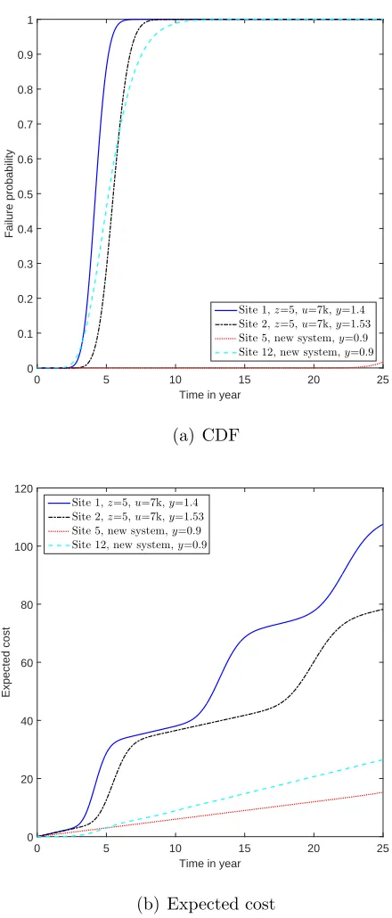
[image:17.595.182.402.155.670.2](b) Expected cost
impact of operating cost increases in dampening the effect of capital replacement costs. If we focus only upon smaller changes in the unit operational cost for one component, say CO = 0.03 to CO = 0.07 for the base setting of CO = 0.05 within the full set of
sensitivity analysis, although all figures are not shown here, then we find that although the absolute values of the expected costs change, their relative profiles do not. Especially in the next 5-year time horizon, we find that the implications for managing assets across the six sites remain the same. Hence within this time window, the results are insensitive to small changes in the operational cost values.
7
Conclusions
This article has developed a cost prediction model for a load-sharing system which has already accrued operational experience and so is a useful extension of the model originally reported in [11]. Our model is developed for a generalization of a problem motivated by the context of a real infrastructure system, specifically for the water treatment process. We believe that the problem definition is also relevant for other infrastructure contexts, such as wind farms and other power plants. Although the particularities of specific contexts will, of course, impact some modeling choices. For example, the nature of key influential factors and their treatment relevant to data availability, as well as the selection of the underlying probability model. The characteristics of the problem - multiple assets, of different ages, located at different sites, different environmental conditions and different rates of degradation - challenge asset management planning. The modeling methodol-ogy developed in this article can be developed to support asset managers address such challenges in the following ways. First, by providing estimates of the expected time of failure and cost of maintenance, the model can provide asset managers with forecasts of spend over defined budget planning horizons. Second, the model has the potential to allow managers to explore the likely impact of investments in other parts of the process to change the workload on key assets and hence impact their degradation failure profile. Finally, the model could be developed to allocate budget.
Scientifically, this article reports method developments associated with the new model. A numerical procedure based on the Riemann-Stieltjes sums has been developed to eval-uate the expected cost. The approximation error is shown to be of order O(n−1). The
model is also able to capture the impact of influential factors on different assets within a portfolio. When these influential factors are observable, we treated them as covariates and incorporated into the CWL-to-failure distribution. When they are unobservable, we treated them as random effects. Statistical inference on the necessary parameters has been developed for both these model variants.
Time in year
0 5 10 15 20 25
Expected cost
0 10 20 30 40 50 60 70 80 90
Site 1,z=5,u=7k,y=1.4
Site 3,z=5,u=7k,y=1.04
Site 8,z=2,uunknown,y=0.4
Site 11,z=1,u=1.5k,y=0.2
Site 13,z=1,u=200,y=0.8 Site 15, new system,y=0.3
(a) CO= 0.01
Time in year
0 5 10 15 20 25
Expected cost
0 50 100 150 200 250
Site 1,z=5,u=7k,y=1.4 Site 3,z=5,u=7k,y=1.04 Site 8,z=2,uunknown,y=0.4 Site 11,z=1,u=1.5k,y=0.2
Site 13,z=1,u=200,y=0.8
Site 15, new system,y=0.3
[image:19.595.183.400.153.666.2](b) CO = 0.25
A
Technical Details
A.1
Proof of Theorem 1
For simplicity, suppose ti, i= 0,1,· · · , n, are equally spaced and let h=ti−ti−1 =τ /n.
Abbreviate F∗(t
i),F(ti), f(ti),m(ti) and m(ti)−m(ti−1) as Fi∗, Fi, fi,mi and ∆mi.
When xis in the interval (ti−1, ti), apply Taylor’s expansion toF(tk−x) atx=ti−1/2
to get
F(tk−x) = Fk−i+1/2−fk−i+1/2(x−ti−1/2) +O(h2),
wherek ≥i.Because f has bounded derivative, we can find a commonM1 such that the
remainder term is no larger than M1h2 for all i. Therefore, we have
Z ti
ti
−1
F(tk−x)dm(x) =Fk−i+1/2∆mi−fk−i+1/2Ii+O(h3),
where Ii = Rti
ti−1(x−ti−1/2)dm(x). Similarly, because m has bounded derivative, we can
find a common M2 such that the remainder is no larger than M2h3, regardless of i. In
addition, ∆mi =O(h) and thus
|Ii| ≤ Z ti
ti−1 h
2dm(x) = ∆mih/2 =O(h
2),
where we can again find a common M3 such that the above remainder term is bounded
byM3h2. Therefore, the renewal function mk given by (5) can be evaluated as
mk =Fk+ k X
i=1
Fk−i+1/2∆mi−fk−i+1/2Ii+O(h3)
. (14)
Apply the above result to m1 to see
m1 =
F1−f1/2I1+O(h3)
1−F1/2
.
Comparing it with (6), it is obvious that m1 −m˜1 = O(h2), and ∆m1 −∆ ˜m1 =O(h2).
Suppose that for 2 ≤ i < j, we have mi−m˜i =O(h),∆mi −∆ ˜mi = O(h2). Based on
(14), we have Equation (15) on the top of the next page.
mj =
Fj +Pj−1k=1Fj−k+1/2∆mk−F1/2mj−1+Pji=1
−fj−i+1/2Ii+O(h3)
1−F1/2
(15)
mj−m˜j =
Pj−1
k=1Fj−k+1/2(∆mk−∆ ˜mk)−F1/2(mj−1−m˜j−1) +
Pj
i=1
−fj−i+1/2Ii+O(h3)
1−F1/2
(16)
∆mj−∆ ˜mj =
Pj−2
k=1∆Fj−k+1/2(∆mk−∆ ˜mk) +F3/2(∆mj−1−∆ ˜mj−1)
1−F1/2
+
Pj−1
i=1
−∆fj−i−1/2Ii+O(h3)
−f1/2Ij
1−F1/2
On the other hand, the numerical approximation of mj is given by (6) as
˜
mj =
Fj +Pj−1k=1Fj−k+1/2∆ ˜mk−F1/2m˜j−1
1−F1/2
,
Therefore, their difference is given by Equation (16), which is O(h) because all the three terms in the numerator areO(h). Since ∆mj−∆ ˜mj = (mj−m˜j)−(mj−1−m˜j−1), we can
have Equation (17), where ∆Fj−k+1/2 =Fj−k+1/2−Fj−k−1/2 and ∆fj−k+1/2 =fj−k+1/2− fj−k−1/2. BecauseF andf are differentiable with bounded derivatives, ∆Fj−k+1/2 =O(h)
and ∆fj−k+1/2 =O(h). Therefore, all the three terms in the numerator of Equation (17)
are O(h2). That is, ∆m
j −∆ ˜mj =O(h2). By induction, we have ∆mj −∆ ˜mj =O(h2)
for j = 1,2,· · · , n.
Similarly, we can apply a first-order Taylor expansion to F∗ and so them∗(t
n) in (4)
can be expressed as
m∗(tn) =F∗(tn) + n X
i=1
Fn−i+1/2∗ ∆mi+O(h)
=F∗(tn) + n X
i=1
Fn−i+1/2∗ (∆ ˜mi+O(h2)) +O(h)
=F∗(tn) + n X
i=1
Fn−i+1/2∗ ∆ ˜mi+O(h).
Therefore, the theorem follows.
A.2
Proof of Lemma 1
Express Z as Z = σU +υ, where U is the standard normal random variable. Then
aZ+b=aσU+aυ+b. This means that aZ+b∼ N(aυ+b, a2σ2). Therefore, according
to Appendix A.2. in [30], we can have (7). On the other hand,
E[ecZ+dΦ(aZ +b)]
=
Z ∞
−∞
1
√
2πσexp
−(z−υ)
2
2σ2 +cz+d
Φ(az+b)dz
= exp
cυ+d+ 1 2c
2σ2 × Z ∞ −∞ 1 √
2πσexp
−(z−υ−cσ
2)2
2σ2
Φ(az+b)dz.
When a = 0, the result is obvious. When a 6= 0, let x = az +b. For both a > 0 and
a < 0, by applying the technique of integration by substitution, the above integral can be simplified as
Z ∞
−∞
1
√
2πaσexp
−(x−b−aυ−acσ
2)2
2(aσ)2
Φ(x)dx.
This is exactly the expectation ofE[Φ(U)] whereU ∼ N(aυ+b+acσ2, a2σ2). According
to (7), the integral is equal to
E[Φ(U)] = Φ
aυ+b+acσ2
√
1 +a2σ2
.
A.3
Derivation of Equation (9)
The CDF ofX can be computed asFX(x) =E
Φ
xpλ/x1
µ−
p λ/x
+ exp
2λ1 µ
·Φ
−xpλ/x1
µ−
p
λ/x .
We have assumed 1/µ∼ N(υ, σ2). Therefore, the above equation can be evaluated based
on Lemma 1. The result is exactly Equation (9).
A.4
Derivation of Equation (12)
The joint PDF of Xi = {Xi1, Xi2,· · · , XiNi} conditional on µ, the fixed yet unknown
random effect for this system, is given by
fXi|µ(xi1, xi2,· · · , xiNi|µ) =
λ
2π Ni/2
×exp
−1
2
λωi1
1
µ2 −Niλ
1
µ +λωi2+ 3ωi3
.
We have assumed that 1/µ ∼ N(υ, σ2). Integrating 1/µ out of the above conditional
joint PDF by using Lemma 2, we have that
fXi =
λ
2π Ni/2
(1 +λωi1σ2)−1/2
×exp
−λωi1υ
2−2N
iλυ−Ni2λ2σ2
2(1 +λωi1σ2) −
1
2(λωi2+ 3ωi3)
.
Taking the logarithm of fXi and then summing over i yields the desired result.
B
Data Used for Example
The following data was used for the illustrative example. Table 1 contains the CWL-to-failure for each component at each of the 15 different sites. Table 2 contains summarized data on the CWL recorded over one year for each site. Table 3 contains data on annual average turbidity as the water quality measure for each site.
Acknowledgment
Table 1: CWL-to-failure for each RGF at each site. The number of rows corresponds to the number of components in each site.
Site 1 2 3 4 5 6 7 8
496 674 632 813 1546 2096 1134 8215 811 637 1215 591 868 1275 1896 4207 652 553 965 605 1077 3943 860 1967 585 748 1034 1115 1589 1348 1425
512 764 813 738 1469 478 561 865 784 1137 521 451 1120 714 1093 411 497 1017 641 1262 604 543 1113 580 810 482 505 1160 1145 1011 417 518 1040 501 942
768 591 932 863
533 285 835
426 436 674 546 672 476 664 588 729 432 657 623 539 397 795 541 673
Site 9 10 11 12 13 14 15
11991 1473 10268 1639 1219 1004 9066 5674 897
5339
Table 2: CWL for each site over a one year period.
Site 1 2 3 4 5
Mean monthly CWL 134.75 68.42 136.83 121.42 5.83 Annual CWL 1617 821 1642 257 430
Site 6 7 8 9 10
Mean monthly CWL 36.83 28.83 64 39.83 37.83 Annual CWL 442 346 768 478 454
Site 11 12 13 14 15
[image:23.595.138.458.589.760.2]Table 3: Average turbidity data for each site.
Site 1 2 3 4 5 6 7 8
Turbidity 1.4 1.53 1.04 1.2 0.9 0.6 0.7 0.4
Site 9 10 11 12 13 14 15
References
[1] Z. Tian and M. J. Zuo, “Health condition prediction of gears using a recurrent neural network approach,” IEEE Transactions on Reliability, vol. 59, no. 4, pp. 700–705, 2010.
[2] W. Wang, “A prognosis model for wear prediction based on oil-based monitoring,”
Journal of the Operational Research Society, vol. 58, no. 7, pp. 887–893, 2007.
[3] W. Wang and A. Christer, “Towards a general condition based maintenance model for a stochastic dynamic system,” Journal of the Operational Research Society, pp. 145–155, 2000.
[4] K. Rafiee, Q. Feng, and D. W. Coit, “Condition-based maintenance for repairable de-teriorating systems subject to a generalized mixed shock model,”IEEE Transactions
on Reliability, vol. 64, no. 4, pp. 1164–1174, 2015.
[5] Q. Sun, Z.-S. Ye, and N. Chen, “Optimal inspection and replacement policies for multi-unit systems subject to degradation,” IEEE Transactions on Reliability, vol. 67, no. 1, pp. 401–413, 2018.
[6] Z.-S. Ye and M. Xie, “Stochastic modelling and analysis of degradation for highly reliable products (with discussion),” Applied Stochastic Models in Business and
In-dustry, vol. 31, no. 1, pp. 16–32, 2015.
[7] S. S. Sutar and U. Naik-Nimbalkar, “Accelerated failure time models for load sharing systems,” IEEE Transactions on Reliability, vol. 63, no. 3, pp. 706–714, 2014.
[8] N. Balakrishnan, N. Jiang, T.-R. Tsai, Y. Lio, and D.-G. Chen, “Reliability infer-ence on composite dynamic systems based on Burr Type-XII distribution,” IEEE
Transactions on Reliability, vol. 64, no. 1, pp. 144–153, 2015.
[9] S. Taghipour and M. L. Kassaei, “Periodic inspection optimization of a k-out-of-n
load-sharing system,” IEEE Transactions on Reliability, vol. 64, no. 3, pp. 1116– 1127, 2015.
[10] J. Xu, Q. Hu, D. Yu, and M. Xie, “Reliability demonstration test for load-sharing systems with exponential and Weibull components,” PloS one, vol. 12, no. 12, p. e0189863, 2017.
[11] Z.-S. Ye, M. Revie, and L. Walls, “A load sharing system reliability model with managed component degradation,”IEEE Transactions on Reliability, vol. 63, no. 3, pp. 721–730, 2014.
[12] M. Cooke, R, Experts in Uncertainty. Oxford University Press, 1991.
[13] Y. Hong and W. Q. Meeker, “Field-failure predictions based on failure-time data with dynamic covariate information,” Technometrics, vol. 55, no. 2, pp. 135–149, 2013.
[15] S. Mercier, C. Meier-Hirmer, and M. Roussignol, “Bivariate Gamma wear processes for track geometry modelling, with application to intervention scheduling,”Structure
and Infrastructure Engineering, vol. 8, no. 4, pp. 357–366, 2012.
[16] Z. Wang and E. A. Elsayed, “Degradation modeling and prediction of ink fading and diffusion of printed images,” IEEE Transactions on Reliability, vol. 67, no. 1, pp. 184–195, 2018.
[17] M. Xie, “On the solution of renewal-type integral equations,” Communications in
Statistics-Simulation and Computation, vol. 18, no. 1, pp. 281–293, 1989.
[18] G. A. Whitmore and F. Schenkelberg, “Modelling accelerated degradation data using Wiener diffusion with a time scale transformation,” Lifetime Data Analysis, vol. 3, no. 1, pp. 27–45, 1997.
[19] C. B. King, Y. Xie, Y. Hong, J. H. Van Mullekom, S. P. DeHart, and P. A. DeFeo, “A comparison of traditional and maximum likelihood approaches to estimating thermal indices for polymeric materials,” Journal of Quality Technology, vol. 50, no. 1, pp. 117–129, 2018.
[20] Y. Zhang and H. Liao, “Analysis of destructive degradation tests for a product with random degradation initiation time,”IEEE Transactions on Reliability, vol. 64, no. 1, pp. 516–527, 2015.
[21] X.-S. Si, W. Wang, C.-H. Hu, and D.-H. Zhou, “Estimating remaining useful life with three-source variability in degradation modeling,”IEEE Transactions on Reliability, vol. 63, no. 1, pp. 167–190, 2014.
[22] J. Son, Q. Zhou, S. Zhou, X. Mao, and M. Salman, “Evaluation and comparison of mixed effects model based prognosis for hard failure,” IEEE Transactions on
Reliability, vol. 62, no. 2, pp. 379–394, 2013.
[23] Y. Duan, Y. Hong, W. Q. Meeker, D. L. Stanley, and X. Gu, “Photodegradation modeling based on laboratory accelerated test data and predictions under outdoor weathering for polymeric materials,” The Annals of Applied Statistics, vol. 11, no. 4, pp. 2052–2079, 2017.
[24] Y. Lin, K. Liu, E. Byon, X. Qian, S. Liu, and S. Huang, “A collaborative learning framework for estimating many individualized regression models in a heterogeneous population,” IEEE Transactions on Reliability, vol. 67, no. 1, pp. 328–341, 2018.
[25] X. Liu and L. C. Tang, “Reliability analysis and spares provisioning for repairable systems with dependent failure processes and a time-varying installed base,” IIE
Transactions, vol. 48, no. 1, pp. 43–56, 2016.
[26] V. Slimacek and B. H. Lindqvist, “Nonhomogeneous poisson process with nonpara-metric frailty and covariates,”Reliability Engineering & System Safety, vol. 167, pp. 75–83, 2017.
[28] T. Bedford, J. Quigley, and L. Walls, “Expert elicitation for reliable system design,”
Statistical Science, pp. 428–450, 2006.
[29] W. Q. Meeker and L. A. Escobar, Statistical Methods for Reliability Data. John Wiey & Sons, 1998.
[30] R. Ranjan and T. Gneiting, “Combining probability forecasts,”Journal of the Royal
![Figure 1: A framework for a load-sharing system with managed component degradationproposed in [11].](https://thumb-us.123doks.com/thumbv2/123dok_us/1354548.89032/4.595.156.441.69.201/figure-framework-load-sharing-managed-component-degradationproposed.webp)