Control Oriented Modelling of a Wind Turbine and
Farm
Sung-ho Hur1 and Bill Leithead2
1
School of Electronics Engineering, Kyungpook National University, South Korea
2Wind Energy & Control, University of Strathclyde, UK
E-mail: [email protected]
Abstract. The Matlab/Simulink model of the Supergen (Sustainable Power Generation and Supply) Wind 5 MW exemplar wind turbine, which has been employed by a number of researchers at various institutions and Universities over the last decade, is improved, especially in speed, to facilitate wind farm modelling. Note that wind farm modelling usually involves duplicating wind turbine models, hence the speed of each turbine model is critical in wind farm modelling. The objective is achieved through various stages, including prewarping, implicit and explicit discretisation, and conversion to C. Simulation results are presented to demonstrate that improvement in speed is significant and that the resulting wind turbine model can be used for wind farm modelling more efficiently. It is important to highlight that improvement in speed is achieved without compromising the complexity of the turbine model; that is, each turbine included in a wind farm is not simplified or compromised.
1. Introduction
The Matlab/Simulink® (Matlab) model of the Supergen (Sustainable Power Generation and Supply) Wind 5 MW exemplar wind turbine was first introduced in [1]. It includes modules of aerodynamics, rotor dynamics, actuator dynamics, tower dynamics, drive-train, generator, etc, and has been updated/improved over the last decade and carefully validated against the high fidelity aero-elastic model, i.e. in DNV-GL Bladed (Bladed), of the same exemplar turbine. A through validation has been carried out a number of times and one of the most recent ones can be found in [2]. The Matlab model has been utilised for various different projects [3, 4], especially within the Supergen Wind Consortium, over the last decade.
Over the last several years, the model has also been utilised for developing wind farm models [5, 6, 7]. Wind farm models usually require the wind turbine model to be duplicated and, in turn, the simulation time could be increased exponentially – this is when each turbine model retains the full dynamics and is not simplified or compromised. Thus far, a wind farm model with more than 10 turbines has been considered impractical due to the simulation speed.
Stiff systems require a more stable “implicit” discretisation method, hence Heun’s method is utilised. Heun’s method is further modified to improve the result. Furthermore, stiff systems are known to potentially become unstable when discretised, which should be taken into account when discretising. This phenomenon is avoided by “prewarping” in advance. Once the model has been optimally discretised to improve the simulation speed, it is converted to C for further improvement. In other words, the model is improved in simulation speed through two stages:
(i) optimal, manual discretisation to prevent the Simulink solver from non-optimally performing numerical integration for simulating the stiff drive-train module.
(ii) and conversion of the model to C, which requires the whole model, not only the drive-train module, to be discretised.
Note that discretisation is required not only to avoid non-optimal numerical integration, but also to facilitate conversion of the model to C; that is, without discretisation, conversion of the model to C cannot be conducted.
Simulation results are presented to demonstrate that improvement in simulation speed due to the optimal discretisation and conversion to C is promising, which makes the model more suitable for wind farm modelling.
In Section 2, the original continuous model of Supergen Wind 5 MW exemplar wind turbine is summarised, indicating various model parameters and variables that are included. The model is discretised and converted to C in Section 3. The simulation results are presented in Section 4, and conclusions are drawn in Section 5.
2. Wind Turbine Model
The parameters and variables used for the wind turbine model reported in this section are first summarised as follows:
BT tower fore-aft damping moment
[Nm]
β pitch angle [rad]
Co out-of-plane bending moment
coef-ficient
η drive-train damping ratio
Cp aerodynamic power coefficient γ∗ drive-train material damping
CT thrust coefficient λ tip speed ratio
Ft thrust force [N] Ω in-plane rotor speed [rad/s]
h tower height [m] ΩR rated in-plane rotor speed [rad/s]
I1 inertia of the low-speed shaft [kg m2] ωe rotating blade edge natural
fre-quency [rad/s]
I2 inertia of the high-speed shaft [kg m2]
ωes stationary blade edge natural
fre-quency [rad/s]
J rotor inertia [kg m2] ωf rotating blade flap natural
fre-quency [rad/s]
JC tower/rotor cross-coupling inertia
[kg m2]
ωf s stationary blade flap natural
fre-quency [rad/s]
JT tower fore-aft inertia [kg m2] φH out-of-plane displacement of hub
[rad]
Ka tower shape factor
KT tower fore-aft stiffness [Nm/rad] φR out-of-plane displacement of rotor
[rad]
MAθR in-plane rotor torque [Nm] ρ density [kg/m
3]
N gearbox ratio θR angular displacement of rotor [rad] R rotor radius [m]
TH hub torque [Nm]
V wind speed [m/s]
2.1. Aerodynamics module
In-plane rotor torque is given by the following equation
MAθR =
1 2ρπV
2R3Cp(λ, β)
λ (1)
where the tip-speed ratio, λ, is defined as
λ= RΩ
V (2)
Out-of-plane rotor torque is given by the following equation
MAφR =
1 2ρπV
2R3C
o(λ, β) (3)
Thrust force is given by
Ft=
1 2ρπV
2R2C
T(λ, β) (4)
The aerodynamic power coefficient,Cp, out-of-plane bending moment coefficient,Co, and thrust
coefficient, CT, are obtained using Bladed. 2.2. Rotor module
The rotor dynamics is modelled by the following equations of motion:
¨
θR=−ω2es[(θR−θH)cosβ−(φR−KaφT)sinβ]cosβ
−ω2f s[(θR−θH)sinβ+ (φR−KaφT)cosβ]sinβ
−(ωe2−ωes2 )(Ω2/Ω2R)(θR−θH) +Mθ/J (5)
J JT −JC2 J JT +KaJ JC
¨
φR=ω2es[(θR−θH)cosβ−(φR−KaφT)sinβ]sinβ
−ω2f s[(θR−θH)sinβ+ (φR−KaφT)cosβ]cosβ
−(ω2f −ωf s2 )(Ω2/Ω2R)(θR−KaθT) +Mφ/J
+ JC/J
JT +KaJC
(KTφT +BTφ˙T −hFT) (6)
J JT −JC2 J JT +KaJ2
¨
φT =−ωes2[(θR−θH)cosβ−(φR−KaφT)sinβ]sinβ
+ωf s2 [(θR−θH)sinβ+ (φR−KaφT)cosβ]cosβ
+ (ωf2−ω2f s)(Ω2/ΩR2)(θR−KaθT)−Mφ/J
− 1
JC+KaJ
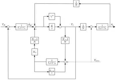
Figure 1: Drive-train module.
The hub torque dynamics is described by the following equation:
TH =J ω2es[(θR−θH)cosβ−(φR−KaφT)sinβ]cosβ
+J ω2f s[(θR−θH)sinβ+ (φR−KaφT)cosβ]sinβ
−J(ωe2−ωes2 )(Ω2/Ω2R)(θR−θH) (8)
Combining (5), (6), (7) and (8), a 6th order nonlinear model can be obtained. 2.3. Drive-train and tower module
The drive-train module is depicted in figure 1. γ∗ in figure 1 denotes drive-train material damping, a function of K1, K2, N, η, I1, and I2. The model depicted in the figure is a fifth order linear equation. The model is stiff causing the Simulink numerical solver to choose a non-optimal, large sampling step, thereby increasing the simulation speed. The model is optimally discretised in Section 3 to improve the speed. As previously mentioned, the model is further improved in speed by converting the discretised module, alongside the rest of the whole model discretised, to C.
2.4. Other dynamics and the turbine controller
The pitch mechanism is modelled using a second order transfer function.
2.5. Validation
This model has been used at various institutions and universities and has been validated thoroughly by various researchers. The most recent validation results using Bladed can be found in [2].
3. Discretisation and Conversion to C
3.1. Discretisation
The continuous model reported in Section 2 includes various modules and dynamics, including aerodynamics module, rotor dynamics module and drive-train module. The drive-train module is stiff and linear. Stiff systems have poles of very different magnitudes, i.e. some poles close to the origin (in the s-plane) and some poles very far away from them, meaning that they contain both slow and fast dynamics. This therefore makes it difficult for the numerical integration solver of Matlab/SIMULNIK to choose a correct and optimal sampling step when simulating the stiff drive-train module, and the solver thus has a strong tendency to opt for a very small sampling step, as opposed to a larger optimal sampling step, resulting in a significant increase in simulation time. This is avoided here by optimally discretising the stiff drive-train module in advance and thereby not requiring numerical integration to be carried out at all during simulation.
The rest of the model, including the aerodynamics and rotors modules, are non-stiff and nonlinear, and the Forward Euler (FE) method is thus used to discretise them. Note that nonlinearity makes it difficult and impractical to utilise implicit discretisation methods, such as Backward Euler or Heun’s method. Fortunately, however, because the modules are non-stiff, the use of “explicit” FE method instead of implicit methods is sufficient in any case.
Moving back on to the drive-train module, the poles that are close to the origin in the s-plane can end up outside the unit circle when discretised, leading to instability. This phenomenon is prevented here by prewarping. Prewarping involves moving the poles of the original continuous drive-train module slightly further away (i.e. to the left) from the origin in the s-plane such that the poles of the discretised drive-train module still remain within the unit circle in the z-plane when discretised. This is achieved here by increasing the material damping of the drive-train module, γ∗.
Since the module is linear, the drive-train module reported in Section 2 can readily be represented in the following standard continuous state space form:
x(t) =Ax(t) +Bu(t)
y(t) =Cx(t) +Du(t) (9)
where x(t) ∈ R5 are the states, y(t) ∈
R2 the drive-train outputs, generator speed and hub speed, and u(t)∈R2 the drive-train inputs, hub torque and generator torque demand.
Since one of the inputs is continuous and the other discrete, (9) is split into two equations, i.e. one with hub torque,u1(t), and the other with torque demand,u2(t). Subsequently, the two equations are discretised differently. By applying Heun’s method to the first one as follows
x(n+ 1) =x(n) +Ts
2 [(Ax(n+ 1) +Bu(n+ 1) +Ax(n) +Bu1(n))] (10)
the following discretised equation is obtained:
x(n+ 1) = (I− Ts
2A)
−1(I +Ts
2 A)
| {z }
E
x(n) + (I−Ts
2 A)
−1Ts
2 B
| {z }
F
u1(n+ 1) (11)
This equation is not in the standard state space form due to the implicit termF u1(n+ 1). This term is, in fact, equivalent to the direct-feed term and hence can be moved to (12) such that
y(n) =Cx¯(n) +CF u1(n) (13)
Note that because the equation has been modified, the state must also be modified from x(n) to ¯x(n). Taking this into account, the following resulting discretised state space model can be derived.
¯
x(n+ 1) =Ex¯(n) + (EF +F)u1(n)
y(n) =Cx¯(n) + (CF +D)u1(n) (14)
Heun’s method essentially allows the module to accept the mean of u(n) and u(n+ 1), i.e. (u(n) +u(n+ 1))/2. This is suitable for u1(t), which comes from another continuous module, aerodynamic module. The other input, u2(t), is received from the discrete controller, and the drive-train module needs to take u2(n) over the sample step instead of the mean. Therefore, (11) is modified for the second input u2(n) as follows.
x(n+ 1) =Ex(n) + 2F u2(n)
y(n) =Cx(n) +Du2(n) (15)
To recapitulate, when the input is aerodynamic torque, which is originally continuous, we use (14), and when the input is generator torque demand, which is discrete from the discrete controller, we use (15). These two models can be combined to obtain one state space equation that accepts both the inputs, hence the model becomes multi-input multi-output (MIMO) as follows.
x(n+ 1) =Ex(n) +Gu(n)
y(n) =Cx(n) +Hu(n) (16)
where u ∈R2, y∈
R2, and x∈R5 denote the same inputs, outputs and states as the original continuous module in (9). Gand H are given as follows:
G=EF1+F1 2F2
(17)
F =F1 F2
(18)
H =
J
1 0
J2 0
(19)
J =
J1 J2T =CF1+D1 (20)
D=D1 D2
(21)
(16) now accepts both aerodynamic torque and generator torque demand producing the outputs of aerodynamic speed and generator speed.
As previously mentioned, the rest modules are non-stiff and nonlinear, so the FE method is used to discretise them. Note that nonlinearity makes it difficult and impractical to utilise implicit discretisation methods, such as Backward Euler or Heun’s method. However, as the modules are non-stiff, the use of an explicit FE method is sufficient anyway. The discretised model of the rest dynamics is combined with that of the drive-train module resulting in the following combined state space model ready for conversion to C:
x(n+ 1) =Ax(n) +Bu(n) (22)
y(n) =Cx(n) +Du(n) (23)
whereu(n)∈R3 are torque demand, pitch demand and wind speed, andy(n)∈
-60 -40 -20 0 20
Magnitude (dB)
10-1 100 101 102
0 180 360 540 720
Phase (deg)
original no prewarping prewarping
Bode Diagram
Frequency (rad/s)
-60 -40 -20 0 20
Magnitude (dB)
10 12 14 16 18 20
0 180 360 540 720
Phase (deg)
original no prewarping prewarping
Bode Diagram
[image:7.595.84.523.126.293.2]Frequency (rad/s)
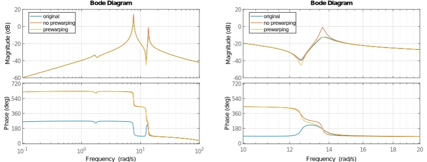
Figure 2: Discretisation and prewarping; the one on the RHS shows a zoomed version.
3.2. Prewarping
Shaft damping is altered prior to discretisation to ensure that the discretised module follows the characteristics of the original continuous module more closely and also to prevent the discretised model from becoming unstable due to the poles close to the y-axis in the s-plane ending up outside the unit circle in the z-plane. Figure 2 depicts the open-loop frequency responses of the wind turbine model including the full envelope controller. The blue plot is the response of the original continuous model and the red plot is the response of the discretised model – as a result of the discretisation described above – without prewarping. The yellow plot is the response of the discretised model that had also been prewarped before it was discretised. The responses in the figure illustrate that the discretised model exhibits more similar characteristics to the original continuous model if it is prewarped in advance. Further, without prewarping the increased peak at around 13.7 rad/s shown in the figure causes the discretised module to become unstable.
3.3. Conversion to C
The continuous model must be discretised to be converted to C, and this is one of the reasons that the model is discretised in Section 3.2 – another reason is to avoid non-optimal numerical integration during simulation as previously mentioned. Once the model has been discretised, it is ready to be converted to C. In more detail, the following procedure is conducted.
(i) The continuous model, including various modules, described in Section 1 is discretised, using the FE and Heun’s methods.
(ii) The discretised model is written in an s-function; that is, the entire model is written in one s-function with all the parameters, inputs and outputs defined in Section 2.
(iii) The discrete s-function is rewritten in C.
(iv) The C file is converted to C MEX for simulation in Matlab/SIMULINK.
4. Simulation Results
100 150 200 250 300 350 400
time 4.2 4.4 4.6 4.8 5 hub torque 106 discrete continuous
100 150 200 250 300 350 400
time 110 115 120 125 generator speed discrete continuous
100 150 200 250 300 350 400
time 0.1 0.15 0.2 0.25 0.3 pitch discrete continuous
100 150 200 250 300 350 400
time -1 -0.5 0 0.5 1 fore-aft acceleration 10-3 discrete continuous
10-1 100 101
Frequency (rad/s) 104 106 108 1010 1012 PSD (Nm 2/rad) hub torque discrete continuous
10-1 100 101
Frequency (rad/s) 10-5 100 105 PSD (Nm 2/rad) generator speed discrete continuous
10-1 100 101
Frequency (rad/s) 10-10 10-5 100 PSD (Nm 2/rad) pitch discrete continuous
10-1 100 101
[image:8.595.115.509.170.582.2]Frequency (rad/s) 10-10 10-9 10-8 10-7 10-6 PSD (Nm 2/rad) FAA discrete continuous
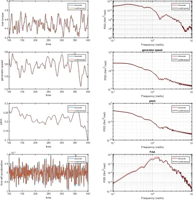
Figure 3: Continuous vs discrete measurements in time and frequency domain.
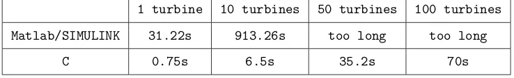
The discretised model from Section 3 is simulated in Matlab/SIMULINK in comparison to the original continuous model for 400 seconds for wind farms of 1, 10 and 100 turbines on an Intel® Core™i7-6700 3.40GHz (8 CPU) machine. The results are shown in table 1. Note that each turbine includes the same commercial full envelope controller that has been discretised in [5] and, and no wind farm controller is included at this stage of the project.
Table 1: Elapsed real time to simulate the continuous and discrete models for 500s
1 turbine 10 turbines 50 turbines 100 turbines
Matlab/SIMULINK 31.22s 913.26s too long too long
C 0.75s 6.5s 35.2s 70s
discrete wind turbine models in the farm model are illustrated in comparison to the original continuous wind turbine model (reported in Section 2) in figure 3. The time and frequency domain responses demonstrate that despite significant improvement in simulation speed, almost identical model outputs are produced; that is, the discretisation of the model and conversion to C results in significant improvement in simulation speed, but the model complexity remains the same.
5. Conclusions
The Matlab model of the Supergen Wind 5 MW exemplar wind turbine, which has been used by various researchers over the last decade, especially within the Supergen Wind Consortium is improved in speed. This is achieved through prewarping, discretisation and conversion to C in order. The optimal discretisation based on Heun’s method prevents the Simulink solver from non-optimally performing numerical integration for simulating the stiff drive-train module, thereby improving the simulation speed. The rest of the model is also discretised (using the FE method) since discretisation is also an essential prerequisite for conversion of the model to C. Subsequently converting the discretised model to C (and then to CMEX for simulation in Matab/SIMULINK) further improves the simulation speed.
As a result, the size of a wind farm model can be increased without increasing the simulation time exponentially in contrast to the original continuous model. The simulation results demonstrate that even with one hundred turbine models included in a wind farm, the simulation speed is 70s. It is important again to emphasise that each turbine model is neither simplified nor compromised.
Acknowledgments
This research was supported by Kyungpook National University Research Fund, 2017. This work was also supported by the EPSRC EP/N006224/1 “Maximising wind farm aerodynamic resource via advanced modelling (MAXFARM)” and FP-ENERGY-2013-IRP GAN-609795 “Integrated Programme on Wind Energy (IRPWind)”.
References
[1] Leithead W and Connor B 2000International Journal of Control 73: 131173 – 1188
[2] Gala-Santos M L 2016Aerodynamic and wind field models for wind turbine control Ph.D. thesis University of Strathclyde
[3] Lei T, Barnes M, Smith S, Hur S, Stock A and Leithead W E 2015IEEE Transactions on Energy Conversion 301043–1051
[4] Chatzopoulos A 2011 Full Envelope Wind Turbine Controller Design for Power Regulation and Tower Load Reduction Ph.D. thesis University of Strathclyde
[5] Poushpas S and Leithead W E 2015International Conference on Renewable Power Generation (RPG 2015) [6] Stock A 2015 Augmented Control for Flexible Operation of Wind Turbines Ph.D. thesis University of
Strathclyde
[7] Hur S and Leithead W E 2016Wind Energy 191667–1686