Rendering Non-Euclidean Space in Real-Time Using Spherical and Hyperbolic Trigonometry

City, University of London Institutional Repository

Citation

:

Child, C. H. T. ORCID: 0000-0001-5425-2308, Osudin, D. and He, Y-H. ORCID:

0000-0002-0787-8380 (2019). Rendering Non-Euclidean Space in Real-Time Using

Spherical and Hyperbolic Trigonometry. Computational Science – ICCS 2019, 19th

International Conference, Proceedings, Part V, 11540, pp. 543-550. doi:

10.1007/978-3-030-22750-0_49

This is the accepted version of the paper.

This version of the publication may differ from the final published

version.

Permanent repository link: http://openaccess.city.ac.uk/id/eprint/22608/

Link to published version

:

http://dx.doi.org/10.1007/978-3-030-22750-0_49

Copyright and reuse:

City Research Online aims to make research

outputs of City, University of London available to a wider audience.

Copyright and Moral Rights remain with the author(s) and/or copyright

holders. URLs from City Research Online may be freely distributed and

linked to.

City Research Online:

http://openaccess.city.ac.uk/

[email protected]

Rendering

Non-Euclidean

Space

in

Real-Time

Using

Spherical

and

Hyperbolic

Trigonometry

DaniilOsudin,Dr ChrisChild,andProfYang-HuiHe

City,UniversityofLondon

Abstract. Weintroduceamethodofcalculatingandrenderingshapes

inanon-Euclidean2Dspaceinreal-timeusinghyperbolicandspherical trigonometry. Werecord theobjects’parameters inapolar coordinate system and use azimuthal equidistant projection to render the space onto the screen.We discussthe complexityof this method, renderings produced, limitationsandpossible applications ofthe createdsoftware aswellaspotentialfuturedevelopments.

Keywords: non-Euclidean geometry·spherical trigonometry·hyperbolic

trigonom-etry·azimuthal equidistant projection·Polar coordinate system·real-time

(a) (b) (c)

Fig. 1.Time-lapse images of multiple objects moving through spherical (a), planar (b)

and hyperbolic (c) 2D space calculated and rendered by the described software

1

Introduction

(b) Planar

(a) Spherical (c) Hyperbolic

Fig. 2.Comparison of parallel lines in the 2D spaces

Non-Euclidean geometry is a field that studies any space that arises from changing Eu-clid’s fifth postulate [1] or changing the metric require-ment. In spherical geometry, Fig. 2 (a), all geodesics

1

r _Θ

A

O Y

x

Fig. 3.Point A with polar

coor-dinatesrandθ

We present a method for calculating the object’s position and its vertices in polar coordinates using spherical [2] or hyperbolic trigonometry [3] [4]. A polar coordinate system of the form (r, θ) is used in this model for all cal-culations instead of Cartesian coordinates. The centre of the of the screen is taken as a refer-ence point O(0,0) for the distance coordinate, r, while eastbound is the reference direction for the bearing coordinate,θ. This allows the same coordinates to be used irrespec-tive of the currect curvature. In order to render the curved space onto a flat 2D screen, we are using azimuthal equidistant projection. By definition, distances and bearing from the centre of the projection are preserved. This works well with Polar coordinates, projection is intuitive and can be used with no changes for both spherical and hyperbolic 2D spaces.

2

Method

ϴ1

V3

V4

r1

C

V2

V1

C’ O O’

Fig. 4. O (0,0), reference

point; C (rc, θc), position and local reference point; Vx (rx, θx), vertices; OO’, refer-ence direction; CC’, local ref-erence direction

The calculations are split into two parts: move-ment of the objects and rendering of the shapes. The screen (rendering space) is limited to a cir-cle of an arbitrary size. When the object’s centre moves past the circumference of the circle, it is repositioned to the antipodal point on the circle with the velocity preserved. This is implemented in order to keep the objects in the visible area on the screen.

Shape has a list of position vectors for each vertex in local coordinates with object’s position being the reference point and reference direction is taken as the reverse of its position vector (Fig. 4).

2.1 Rendering the shape

LetK∈[−1,1]⊂ <s.t.K= 0⇒Euclidean Geometry;

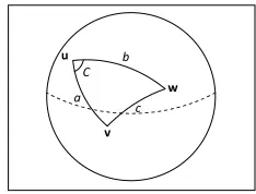
w u

v

b

a c C

Fig. 5.Spherical triangle

K >0⇒Spherical Geometry,r=√1 K

Theorem 1. For a sphere of radius r and

hence Gaussian curvature K = 1

r2 and a

cosc r = cos

a rcos

b r + sin

a rsin

b

rcosC (1)

w u

v

b

a c C

Fig. 6.Hyperbolic triangle

K <0⇒Hyperbolic Geometry,k=−_√1

K

Theorem 2. For a hyperbolic plane with

Gaussian Curvature K = −1

k2 and a

hyper-bolic triangle on its surface described by points

u,vand w, connected by geodesics that form the edges a, b and c, as well as an angle C (Fig. 6), the hyperbolic law of cosines [6] states:

coshc

k = cosh a kcosh

b k−sinh

a ksinh

b

kcosC (2)

Note: To simplify the equations below, all lengths are assumed to have been divided by rorkdepending on the value of K.

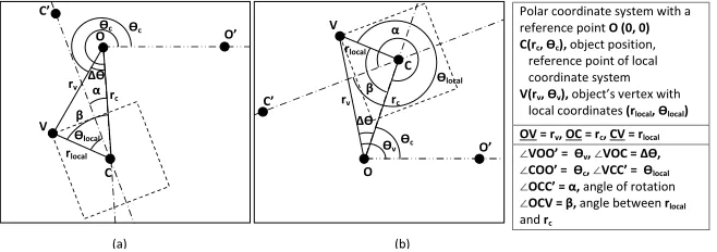
Polar coordinate system with a reference point O (0, 0) C(rc, ϴc), object position,

reference point of local coordinate system

V(rv, ϴv), object’s vertex with

local coordinates (rlocal, ϴlocal)

OV = rv, OC = rc, CV = rlocal ∠VOO’ = ϴv, ∠VOC = Δϴ,

∠COO’ = ϴc, ∠VCC’ = ϴlocal ∠OCC’ = α, angle of rotation

∠OCV = β,angle between rlocal

and rc

ϴc

O ϴc

rv

rc

rlocal

V _ϴβ

local C α Δϴ O’ C’ α Δϴ O C β rc ϴv V rv ϴc ϴlocal C’ O’ rlocal

(a) (b)

Fig. 7. Finding the θ and r coordinates of an object’s vertices through a

hyper-bolic/spherical triangleOCV; Case (a):θlocal+α < π; case (b):θlocal+α > π

Corollary 1. Given: O(0,0), C(rc, θc), V(rv, θv), OC = rc, CV = rlocal,

6 _{COO’ = θc,} 6 _{OCC’ = α,} 6 _{VCC’ = θlocal}

Find:rv,θv = ?

IfK >0, then: If K <0, then:

cosrv= cosrccosrlocal+

sinrcsinrlocalcosβ

coshrv= coshrccoshrlocal−

sinhrcsinhrlocalcosβ

(3)

cos∆θv=

cosrlocal−cosrccosrv sinrcsinrv

cos∆θv=

coshrccoshrv−coshrlocal sinhrcsinhrv

(4)

In order to find rv, first find β = α+θlocal; if Π < β < 2Π, use the

V1 Δϴ2 O C r2 r1 Δϴ1 r1local V2 r2local d rc ϴ1 ϴc ϴ2 (a) (b) V1 d V2 Δϴ2 O’ ϴ2 C r1 ϴ1 ϴc O Δϴ1 rc r1local r2local r2

Polar coordinate system with a reference point O

C(rc, ϴc), object position,

reference point of local coordinate system

V1(r1, ϴ1), object’s vertex 1

V2(r2, ϴ2), object’s vertex 2

OV1 = r1, OV2 = r2, OC = rc, CV1 = r1local, CV2 = r2local,

V1V2 = d, object’s edge

∠V1OO’ = ϴ1,∠V2OO’ = ϴ2,

∠COO’ = ϴc,

∠V1OC = Δϴ1, Δϴ1 = |ϴc - ϴ1|,

∠V2OC = Δϴ2, Δϴ2 = |ϴc - ϴ2|

O’

Fig. 8.Finding the length of edgedand the angle∆θ. Case (a),∆θ1and∆θ2diverge,

so∆θis the sum; case (b), angles converge, so∆θis the absolute value of the difference.

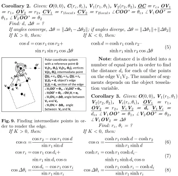
Corollary 2. Given:O(0,0), C(rc, θc), V1(r1, θ1), V2(r2, θ2), OC =rc, OV1

= r1, OV2 = r2, CV1 = r1local, CV2 = r2local, 6 COO’ = θc, 6 V1OO’ =

θ1, 6 V2OO’ = θ2

Find:d,∆θ = ?

If angles converge,∆θ=k∆θ1−∆θ2k; if angles diverge,∆θ=k∆θ1k+k∆θ2k

IfK >0, then: If K <0, then:

cosd= cosr1cosr2+

sinr1sinr2cos∆θ

coshd= coshr1coshr2–

sinhr1sinhr2cos∆θ

(5)

r2 V2

Vi d V1

C ri r1 Δϴi Δϴ

O

ϴ2 ϴi

ϴ1

di

Polar coordinate system with a reference point O

V1(r1, ϴ1), V2(r2, ϴ2), vertices

Vi(ri, ϴi), intermediate point

OV1 = r1, OV2 = r2, OVi = ri,

V1V2 = d, object’s edge

V1Vi = di, section of the edge

∠V1OO’ = ϴ1,∠V2OO’ = ϴ2,

∠ViOO’ = ϴi, ∠OV1Vi = α,

∠V1OV2 = Δϴ,angle between

V1 and V2

∠V1OVi = Δϴi, angle

between V1 and Vi

α

O’

Fig. 9. Finding intermediate points in

or-der to renor-der the edge.

Note: distance d is divided into a number of equal parts in order to find the distance di for each of the points on the edge V1V2. The number of seg-ments depends on the object tessela-tion variable.

Corollary 3. Given:O(0,0), V1(r1, θ1),

V2(r2, θ2), Vi(ri, θi), OV1 = r1,

OV2 = r2, V1V2 = d, V1Vi =

di, 6 V1OO’ = θ1, 6 V2OO’ = θ2,

6 _{V1OV2 = ∆θ}

Find:ri,θi = ?

IfK >0, then: If K <0, then:

cosα=cosr2−cosr1cosd sinr1sind

cosα=coshr1coshd−coshr2 sinhr1sinhd

(6)

cosri= cosr1cosdi+

sinr1sindicosα

coshri = coshr1coshdi–

sinhr1sinhdicosα

(7)

cos∆θi=

cosdi−cosr1cosri sinr1sinri

cos∆θi =

coshr1coshri−coshdi sinhr1sinhri

α is calculated to find the angle opposite ri. Then ri and subsequently ∆θi

can be found using the cosine rule (illustrated on Fig. 9). Then to find actual coordinates of the point Vi, ri should be multiplied by r or k depending on the

value of K; ∆θi should be added to or subtracted from angle θ1, depending on

the direction of the edge d, determined previously.

2.2 Updating object position

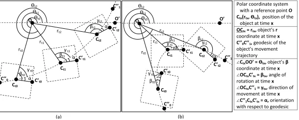
Polar coordinate system with a reference point O Ctx(rtx, ϴtx), position of the

object at time x OCtx = rtx, object’s r coordinate at time x C’’0C’’1, geodesic of the object’s movement trajectory

∠CtxOO’ = ϴtx, object’s β coordinate at time x ∠OCtxC’tx = βtx, angle of rotation at time x ∠OCtxC’’1 = γtx, direction of movement at time x ∠C’’1CtxC’tx = α, orientation with respect to geodesic βt2 ϴt1 ϴt2 ϴt0 rt0 βt0 C’’0 Ct2 O’ βt1 γ t1

O

α

C’t0

C’t1

γ t0

γt2 C’t2 C’’1 rt2 rt1 Ct0 Ct1 α α

(a) (b)

C’t2 Ct1

ϴt1 ϴt2

O ϴt0

rt0 rt1 C’’0 C’t1 βt0 γt2 O’ Ct2 βt2 βt1 γ t1 α

C’’1 α

α γ t0 C’t0

rt2

Ct0

Fig. 10.Movement of the object along a hyperbolic in Spherical (a) and Hyperbolic (b)

space. Orientation with respect to the geodesic is kept the same (angleαis constant) if the object is not rotating.

Corollary 4. Given:O(0,0), Ct0(rt0, θt0), Ct1(rt1, θt1), OCt0 = rt0, Ct0Ct1

= rp, 6 Ct0OO’ = θt0, 6 OCt0C” = γt0, 6 OCt0C’t0 = βt0

Find:rt1,θt1,γt1,βt1 = ?

γt0 should be 0 to π, if calculated value is γt0 > π, take the explemntary

angle. This indicates the movement direction with respect to the reference point. Let6 _{OCt1Ct0 =γt}0₁

IfK >0, then: If K <0, then:

cosrt1= cosrt0cosrp+

sinrt0sinrpcosα

coshrt1= coshrt0coshrp+

sinhrt0sinhrpcosα

(9)

cos∆θ=cosrp−cosrt0cosrt1 sinrt0sinrt1

cos∆θ=coshrt0coshrt1−coshrp sinhrt0sinhrt1

(10)

cosγ_t0₁=cosrt0−cosrpcosrt1 sinrpsinrt1

cosγ_t0₁=coshrpcoshrt1−coshrt0 sinhrpsinhrt1

(11)

α=βt0−γt0.αis the difference between rotation direction and the geodesic

of movement (C”0C”1), it does not change if the object is not rotating. Hence, βt1=γt1+α. Becauseγt01 andγt1 are supplementary angles,γt1=Π−γ0t1.

To find the θ coordinate, either subtract or add ∆θ to the θc depending on

3

Results

3.1 Implementation

Using the method described above and OpenGL, we created a software capable of calculating the objects and rendering the vector graphics in a non-Euclidean space with constant curvature in the range of −1 ≤ K ≤1. Fig. 1 shows the time-lapses of multiple objects in spherical (a), planar (b) and hyperbolic (c) geometries. They show movement through different geodesics at K= 1,K= 0 andK=−1 respectively. Starting positions as well as shape definitions of each object are the same across all time-lapses (grid-lines have been created and rendered as separate objects). The software can calculate the object moving in arbitrary direction with arbitrary speed as well as starting from arbitrary position in the space.

Curvature of the world can be modified in real-time using keyboard inputs in a similar manner to controlling the object’s acceleration and orientation. Another feature is the cut-off of the world at a distance ofNpixels. This can be seen in the hyperbolic and planar time-lapse images. While these spaces should be infinite, we chose to limit them in order to keep objects within the boundaries of the screen (non-shaded area). We created a video [7] displaying the implementation.

3.2 Complexity Analysis

Positions of each vertex need to be calculated, requiringO(v) time, where v is the number of vertices. Subsequently, intermediate points have to be computed, requiring O(i) time to find all of the points on a single edge, where i is the level of tessellation. Complexity to render the world withsnumber of shapes is thereforeO(s∗v∗i). The best case would be equal toO(n) complexity, if two of the terms are negligibly small. The worst case can be approximated toO(n3_{) if} all terms were comparably large. Spatial complexity for shape rendering is only O(v∗i) as previous shape’s data is rewritten to store the next shape’s data. So either O(n) in the best case orO(n2_{) in the worst case.}

Only one movement calculation per object is required and the previous po-sition record is overwritten, both spatial and time complexity is O(n), where n is the number of objects in the world.

Trigonometric and hyperbolic functions in the calculations are slower to com-pute than simpler operations, hence additional cost (implementation dependent). For example the AGM iteration [8] method is faster than the previously common Taylor series method.

4

Discussion

The next step in the project’s development is improving the execution time using parallelised calculations. Subsequent calculation of the points creates a bottleneck, which can be solved by performing some calculations directly on the GPU. Other approaches are considered as well, including lookup tables to speed up trigonometric calculations, for example, Frank Rochet’s implementation [9]; or finding intermediate points from a geodesic equation.

Potential applications for the software include education about non-Euclidean geometry (more intuitive than standard projections: Poincare disk and Upper Half-Plane models); cartography [10] (the engine could be modified to efficiently convert data into different projections); ecology [11] and climatology [12] (mod-elling dynamic systems); Astrophysics (mod(mod-elling systems of cosmological ob-jects and gravitational fields) and video games (game engine for a real-time continuous non Euclidean space, unlike HyperRogue [13], which uses step by step implementation).

References

1. T. L. Heath,Euclid’s Elements. Dover, 1956. (translated).

2. I. Todhunter,Spherical Trigonometry For the use of colleges and schools. Project Gutenberg License, 1886. (republished November 12, 2006).

3. H. S. Carslaw,The Elements of Non-Euclidean Plane Geometry and Trigonometry. Longmans, Green and co., 1916.

4. T. Traver, “Trigonometry in the hyperbolic plane,” 2014 (accessed December 2017). Manuscript.

5. W. Gellert, S. Gottwald, M. Hellwich, H. K¨astner, and H. K¨ustner, The VNR Concise Encyclopedia of Mathematics, 2nd ed.Van Nostrand Reinhold: New York, 1989. ch. 12.

6. J. Gray, Non-euclidean geometry—A re-interpretation. Historia Mathematica, 1979. 236–258.

7. D. Osudin, C. Child, and Y. Hui-He, “Rendering non-euclidean space in real-time using spherical and hyperbolic trigonometry,” 2019. https://youtu.be/A1ZCFh5qfNg.

8. R. P. Brent, “Multiple-precision zero-finding methods and the complex-ity of elementary function evaluation,” 2010 (accessed August 26, 2018). http://arxiv.org/abs/1004.3412v2.

9. F. Rochet, “Fast trigonometry functions using lookup tables,” 2004 (accessed August 30, 2018). http://www.flipcode.com/archives/ Fast Trigonometry Functions Using Lookup Tables.shtml.

10. G. Gartner and H. Huang, “Recent research developments in modern cartography in europe,”Issue 1: EuroCarto 2015, 2015.

11. C. Sutherland, “Modelling non-euclidean movement and landscape connectivity in highly structured ecological networks,”British Ecological Society, 2014.

12. C. Frei, “Interpolation of temperature in a mountainous region using nonlinear profiles and non-euclidean distances,”Royal Meteorological Society, 2013.