EXPLORING THE BENEFITS OF INTERNATIONAL
GOVERNMENT BOND PORTFOLIO DIVERSIFICATION STRATEGIES
Jonathan Fletchera, Krishna Paudyala, Timbul Santosob
a University of Strathclyde b Central Bank of Indonesia
Key Words: International Diversification, International Government Bonds, Bayesian Analysis
JEL Classification: G11, G12
Current draft: February 2018
Address correspondence to Professor J. Fletcher, Department of Accounting and Finance, University of Strathclyde, Stenhouse Building, 199 Cathedral Street, Glasgow, G4 0QU, United Kingdom, phone: +44 (0) 141 548 4963, fax: +44 (0) 552 3547, email:
j.fletcher@strath.ac.uk
2
EXPLORING THE BENEFITS OF INTERNATIONAL
GOVERNMENT BOND PORTFOLIO DIVERSIFICATION STRATEGIES
ABSTRACT
1 I Introduction
Ever since the seminal studies of Grubel(1968) and Solnik(1974), there has been a strong case for international portfolio diversification. The benefits of international diversification have been questioned in recent years due to increased correlations over time especially in developed markets (Goetzmann, Li and Rouwenhorst(2005)). A recent study by Hodrick and Zhang(2014) re-examine the benefits of international diversification in developed equity markets using a variety of different measures and finds that significant international diversification benefits in developed equity markets remains.
Much of the empirical literature on international diversification focuses on equity portfolios. There is a much smaller literature looking at the diversification benefits of bond portfolios. This fact is perhaps surprising given the size of international bond markets. As of March 2015, the amount outstanding of general government international debt securities across all countries is $1,563.4 billion (Bank of International Settlements). Levy and Lerman(1988) find significant diversification benefits for U.S. investors in developed market bond portfolios between 1960 and 1980. The benefits are larger than from international stock portfolios. Eun and Resnick(1994) and Glen and Jorion(1993) find significant benefits of investing in international government bond indexes, especially when currency hedged.
Hansson, Liljeblom and Loflund(2009) examine the benefits of international bond portfolio strategies from a U.S. and a non-U.S. perspective1. They find that there are no significant benefits of investing in developed market government bond portfolios, even when using currency hedging. Using emerging market bond portfolios does lead to significant
1 Studies of international diversification are dependent on the currency chosen. Hentschel
2
benefits but is largely eliminated when investors face no short selling constraints. When international corporate bond portfolios are included in the investment universe, there are significant benefits when the corporate bonds are hedged. Liu(2016) extends the results of Hansson et al(2009) and finds substantial benefits of investing in international corporate bonds. Briere, Mignon, Oosterlinck and Szafarz(2016) take a central bank perspective and examine the benefits of investing in short-term developed government bonds and U.S. non-bond assets such as mortgage backed securities, domestic non-bonds, and equities. Briere et al (2016) find that U.S. non-bond assets are important to increase the portfolio average return. The optimal short-term developed market bonds are useful for reducing portfolio volatility.
We use the Bayesian approach of Wang(1998) to examine the diversification benefits of international government bonds from a U.S. perspective. Our study focuses on two main issues. First, we examine the diversification benefits provided by three types of international government bonds that has not been fully addressed by the prior literature. We consider the benefits of longer maturity G7 government bonds, a global inflation-linked bond index, and emerging markets (EM) bonds based on geographical location and credit rating. We evaluate the diversification benefits as the increase in Certainty Equivalent Return (CER) performance2 for a mean-variance investor of adding the international government bonds to a benchmark investment universe. We consider both unconstrained portfolio strategies, and constrained portfolio strategies, where there are no short selling constraints3.
Second, we examine if the diversification benefits of international government bonds varies across different economic states. We use the dummy variable approach of a given
2 We also consider performance measures based on Value at Risk (VAR) and Conditional
VAR measures developed by Alexander and Baptista(2003).
3 We also examine the impact of a combined upper bound constraint on the emerging market
3
lagged information variable of Ferson and Qian(2004) and Ferson, Hnery and Kisgen(2006) to identify the economic states. Since the short rate is used in most bond pricing models, we use the lagged one-month U.S. Treasury Bill as the information variable. The dummy variable approach allows us to identify months where the lagged Treasury Bill return is lower than normal, normal, and higher than normal. The attraction of the dummy variable approach is that it allocates each month to one of three states using only information prior to that month, rather than ex post indicators such as the NBER recession states.
There are three main findings in our study. First, when only investing in G7 government bond portfolios, no short selling constraints substantially reduces the magnitude but does not eliminate the diversification benefits of the G7 government bonds. Second, when investing in the three groups of international government bonds, there are significant diversification benefits from constrained portfolio strategies. The superior performance is driven by emerging market bonds. Third, the diversification benefits of international government bonds vary across economic states. The strategies deliver their best performance when the lagged one-month U.S. Treasury Bill return is lower than normal. Our results suggest that there are significant diversification benefits of investing in international government bonds.
4
rather than international corporate bonds. Second, we extend the prior evidence of Levy and Lerman(1988), Hansson et al(2009), and Liu(2016) among others by using the dummy variable approach of Ferson and Qian(2004) and Ferson et al(2006) to evaluate the diversification benefits across economic states. We complement Briere et al(2016) who evaluate the diversification benefits in rising interest rate states. We differ from Briere et al by identifying states ex ante rather than ex post. We also apply the dummy variable approach to a different context from conditional mutual fund performance as in Ferson and Qian(2004) and Ferson et al(2006).
The paper is organized as follows. Section II presents the research method used in our study. Section III describes the data. Section IV reports the empirical results and the final section concludes.
II Research Method
We use the mean-variance approach to examine the diversification benefits of the international government bond portfolio strategies4. The mean-variance approach of Markowitz(1952) assumes that investors select a (N,1) vector of risky assets to:
Max x’u – (γ/2)x’Vx (1) where u is a (N,1) vector of expected excess returns, V is a (N,N) covariance matrix of excess returns, and γ is the risk aversion level of the investor. The framework in (1) assumes that the remainder of the portfolio is invested in the risk-free asset (xf) such that x’e + xf = 1, where e is a (N,1) vector of ones. We can include additional constraints to equation (1) such as no short selling (xi ≥ 0, i=1,…,N).
4 A partial list of studies that evaluate the benefits of international diversification using the
5
We conduct our analysis from a U.S. perspective and the domestic investment universe is given by the one-month Treasury Bill and the excess returns of a U.S. domestic government bond index. We consider the diversification benefits of adding three classes of international government bond portfolios to the domestic investment universe:
1. G7 government bond indexes of different maturities.
2. Inflation linked bond – this index is a global government inflation linked bond index. 3. Emerging market bonds – this includes both regional bond indexes and country rating bond indexes.
A number of alternative measures can be used to evaluate the diversification benefits from a mean-variance perspective such as Kandel, McCulloch and Stambaugh(1995), Wang(1998), and Li et al(2003). We measure the diversification benefits using the mean-variance objective function in (1) as the CER performance. The benefits are given as the increase in the CER performance of adding the international government bonds to the domestic investment universe as:
DCER = (x’u – (γ/2)x’Vx) – (xb’u – (γ/2)xb’Vxb) (2) where xb is a (N,1) vector of weights in the benchmark portfolio which is the optimal weight in the benchmark strategy and the remaining (N-1) cells are zero. The DCER measure in equation (2) is the increase in CER performance5 between holding the optimal portfolio in the N risky assets and the optimal benchmark portfolio. If there are no diversification benefits in holding the optimal international government bond portfolio, we expect DCER = 0.
5 The CER performance measure is commonly used to evaluate the performance of
6
We can generalize the DCER measure in equation (2) to also compare the difference in CER performance between two optimal bond portfolios to capture the marginal benefit of adding specific bond indexes to the investment universe. We estimate the DCER measure using two levels of risk aversion, where γ = 1, and 3 as in Tu and Zhou(2011). When including just the G7 government bonds, we consider both unconstrained portfolio strategies and constrained portfolio strategies, where no short selling is allowed in the risky assets and the one-month Treasury Bill. When we include all bonds, we consider two constrained portfolio strategies. First, we impose no short selling constraints in the risky assets and the one-month Treasury Bill. Second, we add a combined upper bound constraint of 20% to the emerging market bonds.
We use the Bayesian approach of Wang(1998) and Li et al(2003) to estimate the increase in CER performance (DCER) and evaluate statistical significance6. An alternative approach to examine the diversification benefits would be to use classical tests of variance efficiency and spanning. Kan and Zhou(2012) provide a review of different mean-variance spanning tests, when the only constraint is the budget constraint. De Roon, Nijman and Werker(2001), Basak, Jagannathan and Sun(2002), and Briere, Drut, Mignon, Oosterlinck and Szafarz(2013) develop asympototic mean-variance spanning and efficiency tests that allows for no short selling constraints.
Li et al(2003) point out that the Bayesian approach has a number of advantages over the asymptotic tests. First, the uncertainty of finite samples is included in the posterior distribution. Second, the Bayesian approach is easier to implement and can include a wide range of portfolio constraints without any additional difficulty and different performance
6 Recent applications of the Bayesian approach include Hodrick and Zhang(2014) and
7
measures can be used. Third, the asymptotic tests rely on a linear approximation to a nonlinear function but the Bayesian approach uses the exact nonlinear function.
The analysis assumes that the N asset excess returns have a multivariate normal distribution7. We assume a non-informative prior about the expected excess returns u and the covariance matrix V. Define us and Vs as the sample moments of the expected excess returns and covariance matrix, and R as the (T,N) matrix of excess returns on the N assets. The posterior probability density function is given by:
p(u,V|R) = p(u|V,us,T)p(V|Vs,T) (3)
where p(u|V,us,T) is the conditional distribution of a multivariate normal (us,(1/T)V) distribution and p(V|Vs,T) is the marginal posterior distribution that has an inverse Wishart(TV, T-1) distribution (Zellner, 1971)).
To approximate the posterior distribution of the DCER measure, we use the Monte Carlo method of Wang(1998). We use the following four-step approach. First, a random V matrix is drawn from an inverse Wishart (TVs,T-1) distribution. Second, a random u vector is drawn from a multivariate normal (us,(1/T)V) distribution. Third, given the u and V from steps 1 and 2, the DCER measure from equation (2) is estimated. Fourth, steps 1 to 3 are repeated 1,000 times to generate the approximate posterior distribution of the DCER measure.
The posterior distribution of the DCER measure is then used to assess the size of the diversification benefits and the statistical significance of these benefits. The average value from the posterior distribution of the DCER measure provides the average diversification
7 We can view the normality assumption as a working approximation to monthly excess
8
benefits in terms of the increase in CER performance. The values of the 5th percentile of the posterior distribution of the DCER measure provides a statistical test of the average DCER = 0 (Hodrick and Zhang(2014)). If the optimal bond portfolios provide significant diversification benefits, we expect to find a significant positive average DCER measure.
The Monte Carlo simulation also gives the approximate posterior distribution of the optimal weights in the bond portfolio strategies. Britten-Jones(1999) and Kan and Smith(2008) derive the sampling distribution of the optimal mean-variance portfolio weights when there are no portfolio constraints. The Bayesian approach provides an approximate posterior distribution of the optimal weights when there are portfolio constraints. We can use the posterior distribution to examine if the average weights in the optimal portfolios are more than two standard errors from zero (Li et al(2003)).
The analysis so far provides a measure of diversification benefits across the whole sample. To examine the conditional diversification benefits, we use the dummy variable approach of Ferson and Qian(2004) and Ferson et al(2006) to allocate each month into one of three economic states using a lagged information variable zt-18, where zt-1 is the value of the lagged information variable at time t-1. We then use the Bayesian approach to evaluate the diversification benefits of the international government bond portfolio strategies in each state. The attraction of the dummy variable approach is that it is straightforward to implement and the states can be identified ex ante by only using data prior to each month9. Ferson et al(2006) point out that another benefit of the dummy variable approach is that it mitigates the spurious regression bias of Ferson, Sarkissian and Simin(2003) of lagged information variables which have a high first-order autocorrelation.
8 An alternative approach could be the regime switching method of Ang and Bekaert(2004). 9 An alternative approach is followed by Briere et al(2016) who identify months of rising
9
We identify the states as follows. First, we calculate xt-1 as zt-1 minus the past average value of zt-1 over the prior sixty months. Second, we also calculate the standard deviation of zt-1 (σ(zt-1)) over the prior sixty months. Third, given the values of xt-1/σ(zt-1), we construct three dummy variables. If xt-1/σ(zt-1) > 1, Dhigh equals one, and Dlow and Dnormal equal zero. If xt-1/σ(zt-1) < -1, Dlow equals one, and Dnormal and Dhigh equal zero. When -1 ≤ xt-1/σ(zt-1) ≤ 1, Dnormal equals one, and Dlow and Dnormal equal zero. The three dummy variables capture when the lagged information variable is lower than normal, normal, and higher than normal.
Using the CER performance to evaluate the diversification benefits is the relevant performance measure for mean-variance investors. However one criticism of using variance as a risk measure is that it does not adequately capture the tail risk of a portfolio strategy10. Value at Risk (VAR) and Conditional VAR (VAR) measures have been proposed to estimate the tail risk of the portfolio11. Alexander and Baptista(2003) propose a Sharpe(1966) type performance measure to evaluate performance based on mean and VAR. They also note that can adapt to using CVAR. Since we assume multivariate normality, we use their mean/VAR and mean/CVAR measure under this assumption (see equation (11) in the Alexander and Baptista(2003) study). Using these measures, we can evaluate whether there is a significant increase in mean/VAR or mean/CVAR performance of adding international government bonds to the domestic investment universe by the Bayesian approach12.
III Data
10We thank the reviewer and the Editor for encouraging us to examine this issue. 11 See Alexander(2009) for a review of modern risk management.
12 We do not consider the impact of using portfolio constraints based on VAR or CVAR in
10
We adopt a U.S. perspective to evaluate the diversification benefits of international government bond portfolios. Our domestic investment universe is the one-month U.S. Treasury Bill returns and the excess returns of the U.S. domestic bond index. We use the Bank of America U.S. Treasury Master index as the domestic bond index. The one-month Treasury Bill return is collected from Ken French’s web site and the Treasury Master index comes from Thompson Financial Datastream.
We consider adding three groups of international government bonds to the domestic investment universe. We use the Bank of America Merrill Lynch international government bond indexes collected from Datastream and the returns are in U.S. dollars and currency unhedged13. The groups include:
1. G7 government bonds
This group includes four G7 government bond indexes with maturities of 1-5 years, 5-7 years (G5-7 5-5-7yr), 5-7-10 years (G5-7 5-7-10yr), and 10+ years (G5-7 10yr+). The sample period for the G7 bonds is January 1986 and September 2016.
2. Inflation-linked bonds
This group includes the Global government inflation-linked bond index (IL). This bond index is available between January 1998 and September 2016.
3. Emerging markets
This group includes three emerging markets bond indexes based on regions and three emerging markets bond indexes based on country rating. The regional indexes include Asia (EM Asia), Europe/Middle East/Africa (EM EU/ME/Afr), and Latin America (EM LA). The three country rating bond indexes include B, BB, and BBB (EM B, EM BB, and EM BBB)
13 Currency hedging tends to have a positive impact on the performance of international bond
11
ratings. The emerging markets bond indexes are available between January 2005 and September 2016.
Table 1 reports summary statistics of the monthly excess returns of the bond indexes over their respective sample periods. The summary statistics include the mean, standard deviation, minimum, and maximum values (%). Table 2 reports the correlations between the bond indexes over their respective sample periods.
Table 1 here Table 2 here
Table 1 shows that there is a wide spread in the average excess returns of the bond indexes. For the G7 government bond indexes, there is an increase in both the mean and volatility as we move to the longer maturity bonds. The average excess returns among the six emerging market bond indexes range between 0.495% (EM-BBB) and 0.787% (EM-BB). The EM B bond index has the highest volatility among the six emerging market bond indexes and the widest range in minimum and maximum monthly excess returns. The volatility of the bond portfolios are considerably lower than the corresponding international equity portfolios.
12
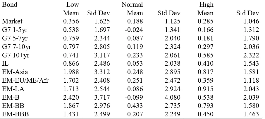
Our study uses the dummy variable approach of Ferson and Qian(2004) and Ferson et al(2006) with the lagged one-month U.S. Treasury Bill return as zt-1. Studies which use a short term interest rate in international asset pricing studies include Harvey(1991), Harvey, Solnik and Zhou(2002), and Zhang(2006) among others. Table 3 reports the mean and standard deviation of the excess bond index returns across the three economic states. Ferson et al(2006) point out that we can estimate the standard error for the difference in mean excess returns in high and low states as 0.05σ(hi)[1+(σ(lo)/σ(hi))2]1/2, where σ(lo) and σ(hi) are the standard deviation of bond excess returns in low and high states.
Table 3 here
Table 3 shows that the international government bonds exhibit substantial variation in mean and volatility across economic states. In contrast, there is little variation in the mean and volatility of the domestic bond index across the three states. The null hypothesis of no significant difference in mean excess returns between the High and Low states cannot be rejected for the domestic bond index. The average excess returns for the international government bonds are highest in the Low state and lowest in the Normal state. In most cases, the volatility of international government bonds is highest in the Low state but the differences in volatility across the three states are more marginal.
13
returns in the Low state suggests that the diversification benefits of the international government bonds might be largest for the Low state.
IV Empirical Results
We begin our analysis by examining the diversification benefits of investing in G7 government bond portfolios. We add to the domestic investment universe, the four G7 government bond indexes with different maturities. Panels A and B of Table 4 report summary statistics of the posterior distribution of the DCER measure (%) for the unconstrained (panel A) and constrained (panel B) portfolio strategies. Panels C and D include the mean and standard deviation of the posterior distribution of the optimal portfolio weights in the unconstrained (panel C) and constrained (panel D) portfolio strategies.
Table 4 here
14
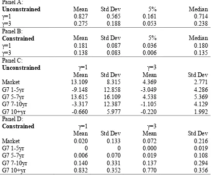
Imposing no short selling constraints leads to a sharp drop in the mean and volatility of the DCER measure in panel B of Table 4. This pattern is similar to Wang(1998) and Li et al(2003) and is due to the lower estimation risk when short selling constraints are imposed (Frost and Savarino(1988) and Jagannathan and Ma(2003))14. The mean DCER measure is significant at the 5% percentile when γ = 1 but is on the borderline of statistical significance when γ = 3. The superior performance of the constrained portfolio strategies in panel B is driven by the large positive average weight on the G7 10+yr index in panel D. The average weight on the G7 10+yr bond index is more than two standard deviations from zero.
Table 4 shows that there are significant diversification benefits of investing in G7 government bonds even in the presence of no short selling constraints. For the constrained portfolio strategies, the benefits are driven by the longest maturity G7 government bonds. Our results differ from Hansson et al(2009) who find no significant benefits of investing in eleven developed market bond indexes, even for unconstrained portfolio strategies. The difference likely stems from a different sample period and the choice of test assets to add to the benchmark investment universe. We use G7 bonds of different maturities rather than the individual developed market bond indexes. Our results also differ from Briere et al(2016). Briere et al find that adding G4 developed market bonds to the domestic investment universe of U.S. government bonds neither significantly increases expected returns nor reduce portfolio volatility. Our results again stand in sharp contrast due to the G7 bonds with longer maturities.
14 Basak et al(2002) find that the standard error of their mean-variance inefficiency measure
15
We next examine whether the diversification benefits of investing in the G7 government bond portfolios varies across economic states. Table 5 reports the summary statistics of the posterior distribution of the DCER measure across the Low (panel A), Normal (panel B), and High (panel C) states. To conserve space, we do not report the mean and volatility of the optimal weights but will discuss in the text.
Table 5 here
Table 5 shows that the diversification benefits of investing in the G7 government bond indexes varies across the economic states. The performance is strongest in the Low state and weakest in the Normal state. Across all three states, there are large significant mean DCER measures using the unconstrained portfolio strategies. The optimal portfolios in the unconstrained strategies have extreme average weights and are highly volatile. None of the average weights in the optimal unconstrained portfolios are more than two standard deviations from zero.
When imposing no short selling constraints, there is a huge drop in the mean and volatility of the DCER measures. In the Normal state, the mean DCER measures are tiny at 0.042% (γ = 3), and 0.06% (γ = 1) and both are insignificant at the 5% percentile. In the High economic state, the mean DCER measures are high relative to the Normal state but the mean DCER measures for both strategies are not significant at the 5% percentile. This finding suggests that no short selling constraints eliminate the diversification benefits of investing in G7 government bond portfolios in Normal and High states.
16
optimal unconstrained portfolios, there are positive average weights on the G7 5-7yr, G7 7-10yr, and G7 10+yr bonds but none are more than two standard deviations from zero. In the constrained portfolio strategies, it is only for the G7 10+yr bond index in the High state that has a large positive average weight more than two standard deviations from zero. The superior performance in the Low state is driven by large positive average weights on the G7 7-10yr and 10+yr bond indexes but the average weights are not more than two standard deviations from zero.
Table 5 shows that the diversification benefits of investing in G7 government bond indexes varies across economic states. It is only in the Low state, that the optimal constrained portfolios deliver significant diversification benefits. We next examine the diversification benefits of adding all three groups of bonds to the domestic investment universe between January 2005 and September 2016. We only report the results for the constrained portfolio strategies using the two models of portfolio constraints. Panels A and B of Table 6 report the summary statistics of the posterior distribution of the DCER measure for the constrained portfolio strategies under the two models of portfolio constraints. Panels C and D report the mean and standard deviation of the posterior distribution of the optimal portfolio weights under the two models of portfolio constraints.
Table 6 here
17
little diversification in the optimal portfolio weights in panel C. The average weight on the EM-BB bond index is close to one and is more than two standard deviations from zero.
Imposing the combined upper bound constraint of 20% on the EM bonds leads to a substantial reduction in the mean and volatility of the DCER measures. However the mean DCER measures remains significant at the 5% percentile for both levels of risk aversion. The optimal weights in panel D show that the EM-BB bond index has the largest average weight among the EM bond indexes and is more than two standard deviations from zero. The largest average weight is now given by the G7 10+yr bond index with smaller average weights in the Market and IL bond index. Neither of the average weights in the Market and IL bond indexes are more than two standard deviations from zero. The average weight on the G7 10+yr index is more than two standard deviations from zero when γ = 1 and borderline when γ = 3.
Table 6 shows that there are significant diversification benefits of investing in the three groups of international government bonds. The superior performance is driven by the EM bonds. This finding is stronger than in Hansson et al(2009), where the diversification benefits of investing in EM bonds depends on the benchmark used when investors face no short selling constraints. The results could differ due to the different time periods and different empirical methods. Hansson et al use the asymptotic test of De Roon et al(2001). Li et al(2003) argue that the Bayesian results are clearer as the uncertainty in finite samples are incorporated into the posterior distribution and the exact nonlinear function is used rather than a first-order approximation in the asymptotic test.
18
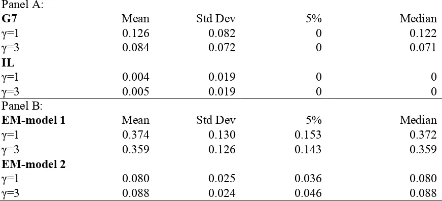
Panel B reports the incremental contribution of the EM bonds for the two models of portfolio constraints.
Table 7 here
Panel A of Table 7 shows that neither the G7 government bonds nor the inflation-linked bond index make a significant incremental contribution to the CER performance when added to the investment universe in the presence of no short selling constraints. The mean DCER measures are small and none are significant at the 5% percentile. In contrast, panel B of Table 7 shows that the EM bonds do make a significant incremental contribution in CER performance under both models of portfolio constraints. When the investor only faces no short selling constraints, the mean DCER measures are large in economic terms and significant at the 5% percentile. Adding the combined upper bound constraint, leads to a sharp drop in the mean and volatility of the DCER measures. However the mean DCER measures remain significant at the 5% percentile. This finding suggests that the EM bonds are the driving force behind the diversification benefits of the international government bond portfolio strategies.
We next examine whether the diversification benefits varies across economic states using all three groups of bonds between January 2005 and September 2016. We use both models of portfolio constraints. Table 8 reports the summary statistics of the posterior distribution of the DCER measure in Low (panel A), Normal (panel B), and High (panel C) economic states.
19
Table 8 shows that the diversification benefits of investing in international government bonds varies across economic states. The diversification benefits are strongest in the Low state and weakest in the Normal state. The mean DCER measures are massive in the Low state and significant at the 5% percentile. Even with the combined upper bound constraint of the EM bonds, the diversification benefits are large. In the High state, the diversification benefits are also highly significant. The mean DCER measures are large in economic terms and significant at the 5% percentile. In contrast, for the Normal state there are no diversification benefits of investing in international government bonds. The mean DCER measures are small and none are significant at the 5% percentile. The results in Table 8 suggest that the constrained portfolio strategies in international government bonds are substantial in states of the world when the lagged one-month U.S. Treasury Bill return is lower and higher than normal.
The final issue we examine is whether the mean-variance strategies deliver significant diversification benefits using mean/VAR and mean/CVAR performance measures. We repeat the tests in Tables 6 and 8 for the constrained portfolio strategies. Table 9 reports summary statistics of the posterior distribution of the alternative performance measures. The results are reported for the January 2005 and September 2016 period (panel A) and for the Low (panel B) and High (panel C) states. We only include the results for the model 1 portfolio constraints as the results are similar when using the combined upper bound constraint on the emerging market bonds. We set the confidence level at t=0.95 and t=0.99 for estimating the mean/VAR and mean/CVAR performance measures.
20
Panel A of Table 9 shows that the diversification benefits of the international government bonds disappears when using the alternative performance measures across the January 2005 and September 2016 period. The average mean/VAR and mean/CVAR measures are small and none are significant at the 5% percentile. There is little difference between the mean/VAR and mean/CVAR measures. Panel A suggests that the superior CER performance in Table 6 comes at the expense of higher VAR and CVAR, which offsets the increase in mean excess returns of investing in the international government bonds.
Panels B and C of Table 9 show that the international government bonds continue to deliver significant diversification benefits in the Low and High states using the alternative performance measures. All of the average mean/VAR and mean/CVAR measures are economically large and significant at the 5% percentile. The magnitude of the benefits is larger in the Low state compared to the High state. Likewise the average mean/VAR measures are larger than the mean/CVAR measures since a portfolio CVAR is higher than the VAR. The results suggests that the diversification benefits in panels A and C in Table 8 are robust to the use of alternative performance measures.
V Conclusions
21
investing in developed market government bonds when the domestic investment universe is U.S. government bonds.
Second, when investing across all three groups of bonds, there are significant diversification benefits using constrained portfolio strategies using the CER measure. This result holds even when investors face a combined upper bound constraint of 20% in EM bonds. The superior performance is driven by the EM bonds, especially the EM-BB index. This finding is stronger than that observed in Hansson et al(2009). The finding complements the results in Li et al(2003) of the diversification benefits of investing in EM equity markets even in the presence of short selling constraints. The significant diversification benefits disappear using the alternative mean/VAR and mean/CVAR measures, which suggests that the increase in the portfolio VAR or CVAR offsets the increase in mean excess returns when investing in international government bonds.
Third, we find that the diversification benefits of international government bond strategies varies across economic states. This result holds whether investing only in the G7 government bonds or in all three groups of bonds. The benefits are strongest in the Low state and poorest in the Normal state. For the constrained portfolio strategies in all international government bonds, there are large and significant diversification benefits when the lagged one-month Tresaury Bill return is both lower and higher than normal. These benefits remain significant using the mean/VAR and mean/CVAR measures. This result suggests that the lagged one-month Treasury Bill return has significant predictive ability of the diversification benefits of international government bond portfolios.
22
23 Table 1 Summary Statistics of Bond Indexes
Bond Mean
Standard
Deviation Minimum Maximum
Market 0.260 1.303 -4.307 5.324
G7 1-5yr 0.195 1.484 -4.219 5.102
G7 5-7yr 0.328 2.127 -5.907 8.448
G7 7-10yr 0.376 2.467 -6.332 8.346
G7 10+yr 0.461 2.508 -6.843 9.295
IL 0.367 2.131 -11.998 7.722
EM-Asia 0.707 2.815 -17.527 14.129
EM-EU/ME/Afr 0.553 2.289 -15.551 7.183
EM-LA 0.580 2.742 -16.371 8.979
EM-B 0.523 3.759 -25.961 9.883
EM-BB 0.787 2.619 -17.795 13.037
EM-BBB 0.495 2.191 -11.123 10.038
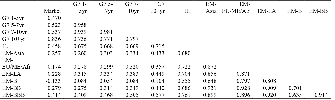
Table 2 Correlations of Bond Indexes
Market G7 1-5yr G7 5-7yr G7 7-10yr 10+yr G7 IL EM-Asia EU/ME/Afr EM-LA EM- EM-B EM-BB G7 1-5yr 0.470
G7 5-7yr 0.523 0.958
G7 7-10yr 0.537 0.939 0.981
G7 10+yr 0.836 0.736 0.771 0.797
IL 0.458 0.675 0.668 0.669 0.715
EM-Asia 0.257 0.260 0.303 0.334 0.433 0.680
EM-EU/ME/Afr 0.174 0.278 0.299 0.320 0.357 0.722 0.872
EM-LA 0.228 0.315 0.334 0.383 0.449 0.704 0.856 0.871
EM-B -0.133 0.084 0.054 0.084 0.104 0.555 0.648 0.797 0.808
EM-BB 0.279 0.275 0.314 0.349 0.442 0.686 0.931 0.928 0.909 0.701
Table 3 Summary Statistics of Bond Indexes in Different Economic States
Bond Low Normal High
Mean Std Dev Mean Std Dev Mean Std Dev
Market 0.356 1.625 0.188 1.125 0.285 1.046
G7 1-5yr 0.538 1.697 -0.024 1.341 0.166 1.312
G7 5-7yr 0.759 2.344 0.087 2.040 0.181 1.790
G7 7-10yr 0.797 2.805 0.119 2.324 0.297 2.036
G7 10+yr 0.741 3.117 0.233 2.061 0.585 2.322
IL 0.866 2.486 0.053 2.038 0.410 1.543
EM-Asia 1.988 3.312 0.248 2.895 0.817 1.581
EM-EU/ME/Afr 1.702 2.408 0.251 2.472 0.359 1.118
EM-LA 1.713 2.544 0.086 2.924 0.915 2.043
EM-B 2.420 3.717 -0.099 4.080 0.538 2.039
EM-BB 1.867 2.976 0.433 2.735 0.793 1.580
EM-BBB 1.431 2.499 0.207 2.249 0.450 1.463
26
Table 4 Posterior Distribution of the DCER Measure: G7 Government Bonds Panel A:
Unconstrained Mean Std Dev 5% Median
γ=1 0.827 0.565 0.161 0.714
γ=3 0.275 0.188 0.053 0.238
Panel B:
Constrained Mean Std Dev 5% Median
γ=1 0.181 0.087 0.036 0.180
γ=3 0.138 0.083 0.006 0.135
Panel C:
Unconstrained γ=1 γ=3
Mean Std Dev Mean Std Dev
Market 13.109 8.315 4.369 2.771
G7 1-5yr -9.148 12.858 -3.049 4.286
G7 5-7yr 13.615 16.109 4.538 5.369
G7 7-10yr -3.317 12.387 -1.105 4.129
G7 10+yr -0.660 5.977 -0.220 1.992
Panel D:
Constrained γ=1 γ=3
Mean Std Dev Mean Std Dev
Market 0.020 0.133 0.072 0.216
G7 1-5yr 0 0 0.000 0.019
G7 5-7yr 0.006 0.070 0.019 0.108
G7 7-10yr 0.140 0.331 0.137 0.294
G7 10+yr 0.832 0.352 0.770 0.356
27
Table 5 Posterior Distribution of the DCER Measure Across Different Economic States: G7 Government Bonds
Panel A: Low
Unconstrained Mean Std Dev 5% Median
γ=1 6.331 3.117 2.127 5.964
γ=3 2.110 1.039 0.709 1.988
Constrained
γ=1 0.470 0.181 0.168 0.464
γ=3 0.417 0.177 0.123 0.412
Panel B: Normal
Unconstrained Mean Std Dev 5% Median
γ=1 2.728 1.528 0.715 2.516
γ=3 0.909 0.509 0.238 0.838
Constrained
γ=1 0.060 0.072 0 0.038
γ=3 0.042 0.061 0 0.012
Panel C: High
Unconstrained Mean Std Dev 5% Median
γ=1 7.681 4.473 1.666 6.831
γ=3 2.560 1.491 0.555 2.277
Constrained
γ=1 0.284 0.189 0 0.283
γ=3 0.243 0.180 0 0.241
[image:29.595.69.514.114.458.2]28
Table 6 Posterior Distribution of the DCER Measure: All Bonds Panel A:
Model 1 Mean Std Dev 5% Median
γ=1 0.505 0.133 0.280 0.505
γ=3 0.449 0.132 0.224 0.450
Panel B:
Model 2 Mean Std Dev 5% Median
γ=1 0.213 0.079 0.090 0.210
γ=3 0.179 0.072 0.078 0.172
Panel C:
Model 1 γ=1 γ=3
Mean Std Dev Mean Std Dev
Market 0.000 0.014 0.000 0.023
G7 1-5yr 0 0 0 0
G7 5-7yr 0 0 0 0
G7 7-10yr 0 0 0 0
G7 10+yr 0.001 0.032 0.005 0.040919
IL 0 0 0 0
EM-Asia 0.054 0.216 0.038 0.171
EM-EU/ME/Afr 0 0 0 0
EM-LA 0.001 0.031 0.001 0.031
EM-B 0.014 0.100 0.005 0.045
EM-BB 0.927 0.239 0.948 0.183
EM-BBB 0 0 0 0
Panel D:
Model 2 γ=1 γ=3
Mean Std Dev Mean Std Dev
Market 0.061 0.202 0.144 0.272
G7 1-5yr 0 0 0 0
G7 5-7yr 0.000 0.015 0.000 0.025
G7 7-10yr 0.002 0.038 0.004 0.051
G7 10+yr 0.670 0.282 0.581 0.313
IL 0.066 0.210 0.068 0.186
EM-Asia 0.011 0.046 0.009 0.042
EM-EU/ME/Afr 0 0 0 0
EM-LA 0 0 0 0
EM-B 0.006 0.033 0.007 0.035
EM-BB 0.181 0.057 0.182 0.054
29
30
Table 7 Posterior Distribution of the Incremental DCER Measures: All Bonds Panel A:
G7 Mean Std Dev 5% Median
γ=1 0.126 0.082 0 0.122
γ=3 0.084 0.072 0 0.071
IL
γ=1 0.004 0.019 0 0
γ=3 0.005 0.019 0 0
Panel B:
EM-model 1 Mean Std Dev 5% Median
γ=1 0.374 0.130 0.153 0.372
γ=3 0.359 0.126 0.143 0.359
EM-model 2
γ=1 0.080 0.025 0.036 0.080
γ=3 0.088 0.024 0.046 0.088
31
Table 8 Posterior Distribution of the DCER Measure Across Economic States: All Bonds Panel A:
Low Mean Std Dev 5% Median
Model 1 γ=1 1.979 0.229 1.609 1.968
γ=3 1.884 0.220 1.535 1.870
Model 2 γ=1 0.808 0.121 0.612 0.806
γ=3 0.770 0.122 0.576 0.769
Panel B:
Normal Mean Std Dev 5% Median
Model 1 γ=1 0.168 0.125 0 0.160
γ=3 0.121 0.107 0 0.096
Model 2 γ=1 0.039 0.028 0 0.038
γ=3 0.038 0.027 0 0.037
Panel C:
High Mean Std Dev 5% Median
Model 1 γ=1 0.735 0.090 0.594 0.737
γ=3 0.704 0.089 0.562 0.704
Model 2 γ=1 0.583 0.079 0.457 0.582
γ=3 0.543 0.078 0.419 0.542
32
Table 9 Posterior Distribution of Alternative Performance Measures: All Bonds
Panel A: All Mean Std Dev 5% Median
Mean/VAR
γ=1.t=0.95 0.074 0.052 -0.011 0.076
γ=3 0.076 0.052 -0.008 0.077
γ=1, t=0.99 0.047 0.033 -0.007 0.048
γ=3 0.048 0.033 -0.005 0.049
Mean/CVAR Mean Std Dev 5% Median
γ=1,t=0.95 0.055 0.038 -0.008 0.056
γ=3 0.056 0.038 -0.006 0.057
γ=1, t=0.99 0.040 0.028 -0.006 0.041
γ=3 0.040 0.028 -0.004 0.041
Panel B: Low Mean Std Dev 5% Median
Mean/VAR
γ=1.t=0.95 0.540 0.124 0.370 0.524
γ=3 0.605 0.147 0.416 0.578
γ=1, t=0.99 0.302 0.061 0.213 0.295
γ=3 0.332 0.067 0.236 0.324
Mean/CVAR Mean Std Dev 5% Median
γ=1,t=0.95 0.364 0.076 0.255 0.356
γ=3 0.403 0.085 0.283 0.390
γ=1, t=0.99 0.247 0.049 0.174 0.241
γ=3 0.271 0.052 0.195 0.265
Panel C: High Mean Std Dev 5% Median
Mean/VAR
γ=1.t=0.95 0.266 0.070 0.157 0.260
γ=3 0.278 0.069 0.179 0.271
γ=1, t=0.99 0.162 0.041 0.097 0.160
γ=3 0.169 0.040 0.110 0.166
Mean/CVAR Mean Std Dev 5% Median
γ=1,t=0.95 0.191 0.049 0.114 0.189
γ=3 0.199 0.048 0.129 0.195
γ=1, t=0.99 0.135 0.034 0.081 0.134
33
34 References
Alexander, G.J., 2009, From Markowitz to modern risk management, European Journal of Finance, 15, 451-461.
Alexander, G.J. and Baptista, A.M., 2003, Portfolio performance evaluation using value at risk, Journal of Portfolio Management, 93-102.
Alexander, G.J. and Baptista, A.M., 2004, A comparison of VaR and CVAR constraints on portfolio selection with the mean-variance model, Management Science, 50, 1261-1273. Alexander, G.J., Baptista, A.M. and S. Yan, 2007, Mean-variance portfolio selection with ‘at-risk’ constraints and discrete distributions, Journal of Banking and Finance, 31, 3761-3781. Ang, A. and G. Bekaert, 2004, How do regimes affect asset allocation?, Financial Analysts Journal, 60, 86-99.
Basak, G., Jagannathan, R. and G. Sun, 2002, A direct test for the mean-variance efficiency of a portfolio, Journal of Economic Dynamics and Control, 26, 1195-1215.
Bekaert, G. and Urias, M.S., 1996, Diversification, integration and emerging market closed-end funds, Journal of Finance, 51 835-869.
Best, M.J. and R.R. Grauer, 2011, Prospect-theory portfolios versus power-utility and mean-variance portfolios, Working Paper, University of Waterloo.
Briere, M., Drut, B, Mignon, V., Oosterlinck, K. and A. Szafarz, 2013, Is the market portfolio efficient? A new test of mean-variance efficiency when all assets are risky, Finance, 34, 7-41. Briere, M., Mignon, V., Oosterlinck, K. and A. Szafarz, 2016, Towards greater diversification in central bank reserves, Journal of Asset Management, 17, 295-312.
Britten-Jones, M., 1999, The sampling error in estimates of mean-variance efficient portfolio weights, Journal of Finance, 54, 655-671.
35
De Roon, F.A., Nijman, T.E. and B.J.M. Werker, 2001, Testing for mean-variance spanning with short sales constraints and transaction costs: The case of emerging markets, Journal of Finance, 56, 721-742.
Ehling, P. and Ramos, S.B., 2006, Geographic versus industry diversification: Constraints matter, Journal of Empirical Finance,13, 396-416.
Eiling, E., Gerard, B., Hillion, P. and F. de Roon, 2012, International portfolio diversification: Currency, industry and country effects revisited, Journal of International Money and Finance, 31, 1249-1278.
Eun, C.S. and B.G. Resnick, 1994, International diversification of investment portfolios: U.S. and Japanese perspectives, Management Science, 40, 140-161.
Ferson, W.E., Henry, T. and D. Kisgen, 2006, Evaluating government bond fund performance with stochastic discount factors, Review of Financial Studies, 19, 423-456. Ferson, W.E. and M. Qian, 2004, Conditional performance evaluation revisited, Research Foundation Monograph, CFA Institute.
Ferson, W.E., Sarkissian S. and T. Simin, 2003, Spurious regressions in financial economics,
Journal of Finance, 58, 1393-1414.
Frost, P.A. and J.E. Savarino, 1988, For better performance: Constrain portfolio weights,
Journal of Portfolio Management, 15, 29-34.
Glen, J. and P. Jorion, 1993, Currency hedging for international portfolios, Journal of Finance, 48, 1865-1886.
Goetzmann, W.N., Li, L. and K.G. Rouwenhorst, 2005, Long-term global market correlations, Journal of Business, 78, 1-38.
36
Grubel, H.G., 1968, International diversified portfolios, American Economic Review, 58, 1299-1314.
Hansson, M., Liljeblom, E. and A. Loflund, 2009, International bond diversification strategies: The impact of currency, country, and credit risk, European Journal of Finance, 15, 555-583.
Harvey, C.R., 1991, The world price of covariance risk, Journal of Finance, 46, 111-157. Harvey, C.R., Solnik, B. and G. Zhou(2002), What determines expected international asset returns?, Annals of Economics and Finance, 3, 249-298.
Hentschel, L., Kang, J. and J.B. Long Jr, 2002, Numeraire portfolio tests of international government bond market integration and redundancy, Working Paper, University of Rochester.
Hodrick, R.J. and X. Zhang, 2014, International diversification revisited, Working Paper, University of Columbia.
Jagannathan, R. and T. Ma, 2003, Risk reduction in large portfolios: Why imposing the wrong constraint helps, Journal of Finance, 58, 1651-1683.
Kan, R. and D. Smith, 2008, The distribution of the sample minimum-variance frontier,
Management Science, 54, 1364-1380.
Kan, R., Wang, X. and G. Zhou, 2017, On the value of portfolio optimization under estmation risk: The case without risk-free asset, Working Paper, University of Toronto. Kan, R. and G. Zhou, 2007, Optimal portfolio choice with parameter uncertainty, Journal of Financial and Quantitative Analysis, 42, 621-656.
Kan, R. and G. Zhou, 2012, Tests of mean-variance spanning, Annals of Economics and Finance, 13, 145-193.
37
Kroll, Y., Levy, H. and H. Markowitz, 1984, Mean-variance versus direct utility maximization, Journal of Finance, 39, 47-61.
Levy, H. and Z. Lerman, 1988, The benefits of international diversification in bonds,
Financial Analysts Journal, 44, 56-64.
Li, K., Sarkar, A. and Z. Wang, 2003, Diversification benefits of emerging markets subject to portfolio constraints, Journal of Empirical Finance, 10, 57-80.
Liu, E.X., 2016, Portfolio diversification and international corporate bonds, Journal of Financial and Quantitative Analysis, 51, 959-983.
Long, J.B. Jr, 1990, The numeraire portfolio, Journal of Financial Economics, 26, 29-69. Markowitz, H., 1952, Portfolio selection, Journal of Finance, 7, 77-91.
Michaud, R.O., 1989, The Markowitz optimization enigma: Is ‘optimized’ optimal, Financial Analysts Journal, 45, 31-42.
Sharpe, W.F., 1966, Mutual fund performance, Journal of Business 39, 119-138.
Solnik, B.H., 1974, Why not diversify internationally rather than domestically?, Financial Analysts Journal, 30, 48-54.
Tu, J. and G. Zhou, 2011, Markowitz meets Talmud: A combination of sophisticated and naïve diversification strategies, Journal of Financial Economics, 99, 204-215.
Wang, Z., 1998, Efficiency loss and constraints on portfolio holdings, Journal of Financial Economics, 48, 359-375.