ON-THE-FLY COMPUTATION OF BISIMILARITY DISTANCES∗
GIORGIO BACCI, GIOVANNI BACCI, KIM G. LARSEN, AND RADU MARDARE Dept. of Computer Science, Aalborg University, Denmark
e-mail address: {grbacci, giovbacci, kgl, mardare}@cs.aau.dk
Abstract. We propose a distance between continuous-time Markov chains (CTMCs) and study the problem of computing it by comparing three different algorithmic methodologies: iterative, linear program, and on-the-fly.
In a work presented at FoSSaCS’12, Chen et al. characterized the bisimilarity distance of Desharnais et al. between discrete-time Markov chains as an optimal solution of a linear program that can be solved by using the ellipsoid method. Inspired by their result, we propose a novel linear program characterization to compute the distance in the continuous-time setting. Differently from previous proposals, ours has a number of constraints that is bounded by a polynomial in the size of the CTMC. This, in particular, proves that the distance we propose can be computed in polynomial time.
Despite its theoretical importance, the proposed linear program characterization turns out to be inefficient in practice. Nevertheless, driven by the encouraging results of our previous work presented at TACAS’13, we propose an efficient on-the-fly algorithm, which, unlike the other mentioned solutions, computes the distances between two given states avoiding an exhaustive exploration of the state space. This technique works by successively refining over-approximations of the target distances using a greedy strategy, which ensures that the state space is further explored only when the current approximations are improved.
Tests performed on a consistent set of (pseudo)randomly generated CTMCs show that our algorithm improves, on average, the efficiency of the corresponding iterative and linear program methods with orders of magnitude.
Introduction
Continuous-time Markov chains (CTMCs) are one of the most prominent models in perfor-mance and dependability analysis. They are exploited in a broad range of applications, and constitute the underlying semantics of many modeling formalisms for real-time probabilistic systems such as Markovian queuing networks, stochastic process algebras, and calculi for systems biology. An example of CTMC is presented in Figure 1(left). Here, states1 goes to
Key words and phrases: Markov chains, Continuous-time Markov chains, behavioral distances, on-the-fly algorithm, probabilistic systems.
∗An earlier version of this paper appeared as [BBLM13]. The present version extends [BBLM13] by considering the case of CTMCs and improves the linear programming approach of [CvBW12].
Work supported by Sapere Aude: DFF-Young Researchers Grant 10-085054 of the Danish Council for Independent Research, by the VKR Center of Excellence MT-LAB and by the Sino-Danish Basic Research Center IDEA4CPS. .
LOGICAL METHODS
lIN COMPUTER SCIENCE DOI:10.23638/LMCS-13(2:13)2017
c
G. Bacci, G. Bacci, K. G. Larsen, and R. Mardare
CC
states3ands4 with probability 13 and 23, respectively. Each state has an associatedexit-rate
representing the rate of an exponentially distributed random variable that characterizes the residence-time in the state1. For example, the probability to move froms1 to any other state
within time t ≥0 is given by R0t3e−3xdx= 1−e−3t. A state with no outgoing transitions (ass3 in Figure 1) is calledabsorbing, and represents a terminating state of the system.
A key concept for reasoning about the equivalence of probabilistic systems is Larsen and Skou’s probabilistic bisimulation for discrete-time Markov chains (MCs). This notion has been extended to several types of probabilistic systems, including CTMCs. In Figure 1(left)
s4 and s5 are bisimilar. Moreover, although s1 and s2 move with different probabilities to
statess4 and s5, their probabilities to reach any bisimilarity class is the same, so that, also
s1 and s2 are bisimilar.
However, when the numerical values of probabilities are based on statistical sampling or subject to error estimates, any behavioral analysis based on a notion of equivalence is too fragile, as it only relates processes with identical behaviors. This issue is illustrated in Figure 1(right), where the states t1 and t2 (i.e., the counterparts of s1 and s2, respectively,
after a perturbation of the transition probabilities) are not bisimilar. A similar situation occurs considering perturbations on the exit-rates or on associated labels, if one assumes they are taken from a metric space.
This is a common issue in applications such as, systems biology [TK10], planning [CP11], games [CdAMR10], or security [CG09], where one is interested in knowing whether two processes that may differ by a small amount in the real-valued parameters (probabilities, rates, etc.) have “sufficiently” similar behaviors. This motivated the development of the metric theory for probabilistic systems, initiated by Desharnais et al. [DGJP04] and greatly developed and explored by De Alfaro, van Breugel, Worrell, and others [dAMRS07, vBW06, vBSW08]. It consists in proposing a bisimilarity distance (pseudometric), which measures the behavioral similarity of two models. These pseudometrics, e.g., the one proposed by Desharnais et al., are parametric in a discount factor that controls the significance of the future in the measurements.
Since van Breugel et al. have presented a fixed point characterization of the aforemen-tioned pseudometric in [vBW01], several iterative algorithms have been developed in order
1Note that the only residence time distributions that ensure the Markov property (a.k.a., memoryless
transition probability) are exponential distributions.
s2
3
s1
3 s3
s4
5
s5
5
1 3 1 3
1 3 1
3
2 3
1 1
t2
3
t1
3 t3
t4
5
t5
5
1 3 1 3
1 3 1
3+ε
2 3−ε
[image:2.612.114.500.555.654.2]1 1
to compute its approximation up to any degree of accuracy [FPP04, vBW06, vBSW08]. Re-cently, Chen et al. [CvBW12] proved that, for finite MCs with rational transition function, the bisimilarity pseudometrics can be computed exactly in polynomial time. The proof con-sists in describing the pseudometric as the solution of a linear program that can be solved using theellipsoid method. Although the ellipsoid method is theoretically efficient, “compu-tational experiments with the method are very discouraging and it is in practice by no means a competitor of the, theoretically inefficient, simplex method”, as stated in [Sch86]. Unfortu-nately, in this case the simplex method cannot be used to speed up performances in practice, since the linear program to be solved may have an exponential number of constraints in the number of states of the MC.
In this paper, we introduce a bisimilarity pseudometric over CTMCs that extends that of Desharnais et al. over MCs, and we consider the problem of computing it both from a the-oretical and practical point of view. We show that the proposed distance can be computed in polynomial time in the size of the CTMC. This is obtained by reducing the problem of computing the distance to that of finding an optimal solution of a linear program that can be solved using the ellipsoid method. Notably, differently from the proposal in [CvBW12], our linear program characterization has a number of constraints that is bounded by a poly-nomial in the size of the CTMC. This, in particular, allows one to avoid the use of the ellipsoid algorithm in favor of the simplex or the interior-point methods.
However, also in this case, the linear program characterization turns out to be inefficient in practice, even for small CTMCs. Nevertheless, supported by the encouraging results in our previous work [BBLM13], we propose to follow an on-the-fly approach for computing the distance. This is inspired by an alternative characterization of the bisimilarity pseu-dometric based on the notion of coupling structure for a CTMC. Each coupling structure is associated with a discrepancy function that represents an over-approximation of the dis-tance. The problem of computing the pseudometric is then reduced to that of searching for anoptimal coupling structure whose associated discrepancy coincides with the distance. The exploration of the coupling structures is based on a greedy strategy that, given a cou-pling structure, moves to a new one by ensuring an actual improvement of the current discrepancy function. This strategy will eventually find an optimal coupling structure. The method is sound independently from the initial starting coupling structure. Notably, the moving strategy is based on a local update of the current coupling structure. Since the update is local, when the goal is to compute the distance only between certain pairs of states, the construction of the coupling structures can be done on-the-fly, delimiting the exploration only on those states that are demanded during the computation.
The efficiency of our algorithm has been evaluated on a significant set of randomly generated CTMCs. The results show that our algorithm performs orders of magnitude better than the corresponding iterative and linear program implementations. Moreover, we provide empirical evidence that our algorithm enjoys good execution running times.
ensuring that the local optimum corresponds to the global one. Our methods can also be used in combination with approximation techniques as, for instance, to provide a least over-approximation of the behavioral distance given over-estimates of some particular distances.
Synopsis: The paper is organized as follows. In Section 1, we recall the basic preliminaries on continuous-time Markov chains and define the bisimilarity pseudometric. Section 2 is devoted to the analysis of the complexity of the problem of computing such a distance. Here, two approaches are considered: an approximate iterative method and a linear program characterization. In Section 3, we provide an alternative characterization of the distance based on the notion of coupling structure. This is the basis for the development of an on-the-fly algorithm (Section 5) for the computation of the pseudometric, whose correctness and termination is proven in Section 4. The efficiency of this algorithm is supported by experimental results, shown in Section 6. Final remarks and conclusions are in Section 7.
1. Continuous-time Markov Chains and Bisimilarity Pseudometrics
We recall the definitions of (finite) L-labelled continuous-time Markov chains (CTMCs) for a nonempty set of labels L, and stochastic bisimilarity over them. Then, we introduce a
behavioral pseudometric over CTMCs to be considered as a quantitative generalization of stochastic bisimilarity.
Given a finite setX, a discrete probability distribution over it is a functionµ:X→[0,1] such that µ(X) = 1, whereµ(E) = Px∈Eµ(x), for E ⊆ X. We denote the set of finitely supported discrete probability distributions over X by D(X).
Definition 1.1 (Continuous-time Markov chain). An L-labelled continuous-time Markov chain is a tuple M = (S, A, τ, ρ, ℓ) consisting of a nonempty finite set S of states, a set
A ⊆S of absorbing states, a transition probability function τ:S\A→ D(S), an exit rate
function ρ:S\A→R>0, and alabeling function ℓ:S →L.
The labels inLrepresent properties of interest that hold in a particular state according to the labeling functionℓ:S →L. Ifs∈S is the current state of the system andE⊆S is a subset of states, τ(s)(E)∈[0,1] corresponds to the probability that a transition fromsto arbitrarys′ ∈E is taken, andρ(s)∈R
>0 represents the rate of an exponentially distributed
random variable that characterizes the residence time in the state sbefore any transition is taken. Therefore, the probability to make a transition from state sto anys′ ∈E within time unitt∈R≥0 is given byτ(s)(E)·exp[ρ(s)]([0, t)), where exp[r](B) =RBre−rx dx, for
any Borel subset B ⊆ R≥0 and r > 0. Absorbing states in A ⊆ S are used to represent termination or deadlock states. An example of a CTMC is shown in Figure 1.
For discrete-time Markov chains, the standard notion of behavioral equivalence is prob-abilistic bisimulation of Larsen and Skou [LS91]. The following definition extends it to CTMCs. To ease the notation, for E ⊆S, we introduce the relation ≡E ⊆S×S defined by s≡E s′ if either s, s′ ∈E or s, s′∈/ E.
Definition 1.2 (Stochastic Bisimulation). Let M= (S, A, τ, ρ, ℓ) be a CTMC. An equiva-lence relation R⊆S×S is astochastic bisimulation on Mif whenever s R t, then
(i) s≡At,ℓ(s) =ℓ(t), and
(ii) ifs, t6∈A, thenρ(s) =ρ(t) and, for all C ∈S/R,τ(s)(C) =τ(t)(C).
Intuitively, two states are bisimilar if they have the same labels, they agree on being absorbing or not, and, in the case they are non-absorbing, their residence-time distributions and probability of moving by a single transition to any given class of bisimilar states is always the same. As an example of two stochastic bisimilar states, considers1ands2in the CTMC
depicted on the left hand side of Figure 1. A bisimulation relation that relates them is the equivalence relation with equivalence classes given by {s1, s2},{s3}, and {s4, s5}.
1.1. Bisimilarity Pseudometrics on CTMCs. In this section, we introduce a family of pseudometrics on CTMCs parametric in a discount factorλ∈(0,1). Following the approach of [vBHMW07], given a CTMCM= (S, A, τ, ρ, ℓ) we define a (1-bounded) pseudometric on
S as the least fixed point of an operator on the set [0,1]S×S of functions fromS×S to [0,1]. This pseudometric is then shown to be adequate with respect to stochastic bisimilarity: we prove that two states are stochastic bisimilar if and only if they have distance zero.
Recall thatd:X×X → R≥0 is a pseudometric on a set X if d(x, x) = 0 (reflexivity),
d(x, y) = d(y, x) (symmetry) and d(x, y) +d(y, z) ≥ d(x, z) (triangular inequality), for arbitraryx, y, z∈X; it is ametric if, in addition,d(x, y) = 0 iffx=y. A pair (X, d) where
dis a (pseudo)metric on X is called a(pseudo)metric space.
Hereafter we will assumeL to be equipped with a 1-bounded metric2 dL:L×L→ [0,1]. The operator we are going to introduce will use three key ingredients: the distance
dL between labels, a distance between residence-time distributions, and a distance between transition distributions. The first is meant to measure thestatic differences with respect to the labels associated with the states, the last two are meant to capture the differences in the
dynamics, respectively, with respect to the continuous and discrete probabilistic choices. To this end, we consider two distances over probability distributions. The first one is thetotal variation metric, defined for arbitrary Borel probability measuresµ, ν over R≥0as
kµ−νkTV = supE|µ(E)−ν(E)|,
where the supremum is taken over the Borel measurable sets of R≥0. The second one is theKantorovich distance, which is based on the notion of coupling of probability measures, which we introduce next in the case of probability distributions over finite sets.
Definition 1.3 (Coupling). Let S be a finite set, and let µ, ν ∈ D(S). A probability distributionω ∈ D(S×S) is said a coupling for (µ, ν) if, for arbitraryu, v∈S
P
v∈Sω(u, v) =µ(u) and
P
u∈Sω(u, v) =ν(v).
In other words,ωis a joint probability distribution with left and right marginal, respectively, given by µand ν. We denote the set of couplings for (µ, ν) by Ω(µ, ν).
For a finite setS and a 1-bounded distance d:S×S→ [0,1] over it, theKantorovich distance is defined, for arbitrary distributionsµ, ν ∈ D(S) as follows3
Kd(µ, ν) = min{Pu,v∈Sd(u, v)·ω(u, v)|ω ∈Ω(µ, ν)}.
Intuitively, Kd lifts a (1-bounded) distance over S to a (1-bounded) distance over its prob-ability distributions. One can show that Kd is a (pseudo)metric if dis a (pseudo)metric.
Now, consider the following functional operator.
2Since the setSof states is assumed to be finite, one may assume the set of labels to be so as well. Thus,
the metricdLon labels can be bounded without loss of generality.
3The minimum can be used in place of an infimum thanks to the Fenchel-Rockafeller duality theorem
Definition 1.4. Let M= (S, A, τ, ρ, ℓ) be CTMC and λ ∈ (0,1) a discount factor. The function ∆Mλ : [0,1]S×S →[0,1]S×S is defined as follows, ford:S×S →[0,1] and s, t∈S
∆Mλ (d)(s, t) =
1 if s6≡At
L(s, t) if s, t∈A
max{L(s, t), λ· T(d)(s, t)} if s, t /∈A
where T : [0,1]S×S →[0,1]S×S and L,E:S×S →[0,1] are respectively defined by
T(d)(s, t) =E(s, t) + (1− E(s, t))· Kd(τ(s), τ(t)),
L(s, t) =dL(ℓ(s), ℓ(t)), and E(s, t) =kexp[ρ(s)]−exp[ρ(t)]kTV. The functional ∆M
λ measures the difference of two states with respect to: their labels (by means of the pseudometric L), their residence-time distributions (by means of the pseudometricE), and their discrete probabilities to move to the next state (by means of the Kantorovich distance). If two states disagree on being absorbing (or not) they are considered incomparable, and their distance is set to 1. If both states are absorbing, they express no dynamic behavior, hence they are compared statically, and their distance corresponds to that occurring between their respective labels. Finally, if the states are non-absorbing, then they are compared with respect to both their static and dynamic features, namely, taking the maximum among their respective associated distances.
Specifically, the value E(s, t) corresponds to the least probability that two transitions are taken independently from the states s and tat different moments in time. This value is used by the functional T to measure the overall differences that might occur in the dynamics of the two states in combination with the Kantorovich distance between their transition probability distributions (see Remark 1.10 for more details).
The set [0,1]S×Sis endowed with the partial order⊑defined asd⊑d′iffd(s, t)≤d′(s, t) for all s, t ∈ S and it forms a complete lattice. The bottom element 0 is the constant 0 function, while the top element is the constant 1 function. For any subset D ⊆ [0,1]S×S, the least upper bound FD, and greatest lower bound dD are, respectively, given by (FD)(s, t) = supd∈Dd(s, t) and (dD)(s, t) = infd∈Dd(s, t), for alls, t∈S.
It is easy to check that, for any M and λ ∈ (0,1), ∆Mλ is monotone (i.e., whenever
d⊑d′, then ∆Mλ (d) ⊑∆Mλ (d′)), thus, since ([0,1]S×S,⊑) is a complete lattice, by Tarski’s fixed point theorem ∆Mλ admits least and greatest fixed points.
Definition 1.5 (Bisimilarity distance). LetMbe a CTMC and λ∈(0,1). Theλ -discoun-tedbisimilarity pseudometric on M, denoted by δMλ , is the least fixed point of ∆Mλ .
The rest of the section is devoted to show that the least fixed pointδλMis indeed a pseu-dometric and, moreover, is adequate with respect to stochastic bisimilarity (Theorem 1.9). This justifies the definition above. To this end we need some technical lemmas. In particu-lar, we prove that ∆Mλ preserves pseudometrics (Lemma 1.6) and it is Lipschitz continuous (Lemma 1.7).
Hereafter, unless mentioned otherwise, we fix a CTMC M = (S, A, τ, ρ, ℓ) and a dis-count factor λ∈(0,1). To ease the notation ∆M
λ ,δMλ , and ∼M will be denoted simply by ∆λ,δλ, and ∼, respectively, whenever Mis clear from the context.
Lemma 1.6. The operator ∆λ preserves pseudometrics.
maximum of pseudometrics is a pseudometric, it suffices to prove that T preserves pseu-dometrics. Recall that, Kd:D(S)× D(S) → [0,1] is a pseudometric, since d is so. Thus, reflexivity and symmetry are immediate. The only nontrivial case is the triangular inequal-ity. Let s, t, u ∈ S \A, we want to prove T(d)(s, t) ≤ T(d)(s, u) +T(d)(u, t). First note that, for 0≤β ≤1 andα′ ≥α, the following holds:
α+ (1−α)β =β+ (1−β)α (distributivity)
≤β+ (1−β)α′ (α≤α′ and 0≤β≤1) =α′+ (1−α′)β . (distributivity) Thus, sinceE is a pseudometric, by triangular inequality and the above we have
T(d)(s, t) =E(s, t) + (1− E(s, t))· Kd(τ(s), τ(t)) (def. T)
≤ E(s, u) +E(u, t) + 1−(E(s, u) +E(u, t))· Kd(τ(s), τ(t)) (∗) If we show that the last summand in (∗) is less than or equal to the sum of (1− E(s, u))·
Kd(τ(s), τ(u)) and (1− E(u, t))· Kd(τ(u), τ(t)), we get the following, and we are done
≤ E(s, u) + (1− E(s, u))· Kd(τ(s), τ(u)) +E(u, t) + (1− E(u, t))· Kd(τ(u), τ(t)) =T(d)(s, u) +T(d)(u, t). (def. T) To this end, consider two cases. If E(s, u) +E(u, t)>1 then the inequality holds trivially, since 1−(E(s, u)+E(u, t))<0, so that the last summand in (∗) is negative and 1−E(s, u)≥0. Instead, ifE(s, u) +E(u, t)≤1 then 1−(E(s, u) +E(u, t))≥0, so we have
1−(E(s, u) +E(u, t))· Kd(τ(s), τ(t))
≤ 1−(E(s, u) +E(u, t))· Kd(τ(s), τ(u)) +Kd(τ(u), τ(t)) (triang. Kd) = 1−(E(s, u) +E(u, t))· Kd(τ(s), τ(u)) + 1−(E(s, u) +E(u, t))
· Kd(τ(u), τ(t))
≤ 1− E(s, u)· Kd(τ(s), τ(u)) + 1− E(u, t)
· Kd(τ(u), τ(t)) and we are done.
The set [0,1]S×S can be turned into a metric space by means of the supremum norm
kd−d′k= sups,t∈S|d(s, t)−d′(s, t)|. Next we show that theλ-discounted functional operator ∆λ isλ-Lipschitz continuous, that isk∆λ(d′)−∆λ(d)k ≤λ·kd′−dk, for anyd, d′ ∈[0,1]S×S.
Lemma 1.7. The operator ∆λ is λ-Lipschitz continuous.
Proof. By [vB12, Corollary 1], to prove that ∆λ isλ-Lipschitz continuous it suffices to show that, whenever d ⊑ d′ then, for all s, t ∈ S, ∆λ(d′)(s, t)−∆λ(d)(s, t) ≤ λ· kd′ −dk. If
s6≡A t, then ∆λ(d′)(s, t)−∆λ(d)(s, t) = 1−1 = 0, so that, the inequality is satisfied. If
s, t /∈ A, ∆λ(d′)(s, t)−∆λ(d)(s, t) = L(s, t)− L(s, t) = 0, and again the inequality holds trivially. The same happens when L(s, t) ≥ λ· T(d′)(s, t). Indeed, by monotonicity of T,
L(s, t)≥λ· T(d)(s, t) holds, so that, by definition of ∆λ we have ∆λ(d′)(s, t)−∆λ(d)(s, t) =λ· L(s, t)− L(s, t)
It remains the case whens, t /∈A and λ· T(d)(s, t) ≤ L(s, t)< λ· T(d′)(s, t). Assume that
Kd(τ(s), τ(t)) =Pu,v∈Sd(u, v)·ω(u, v), for some ω∈Ω(τ(s), τ(t)), then we have ∆λ(d′)(s, t)−∆λ(d)(s, t)≤λ· T(d′)(s, t)− T(d)(s, t)
≤λ· Kd′(τ(s), τ(t))− Kd(τ(s), τ(t))
≤λ· Pu,v∈Sd′(u, v)·ω(u, v)−
P
u,v∈Sd(u, v)·ω(u, v)
=λ· Pu,v∈S(d′(u, v)−d(u, v))·ω(u, v)
≤λ· Pu,v∈Skd′−dk ·ω(u, v)
=λ· kd′−dk ·Pu,v∈Sω(u, v) =λ· kd′−dk.
It is standard that [0,1]S×S with the supremum norm forms a complete metric space (i.e, every Cauchy sequence converges). Therefore, since λ∈(0,1), a direct consequence of
Lemma 1.7 and Banach’s fixed point theorem is the following.
Theorem 1.8. For any λ∈ (0,1), δλ is the unique fixed point of ∆λ. Moreover, for any
n∈N, and d:S×S →[0,1]we have kδλ−∆nλ(d)k ≤ λ n
1−λk∆λ(d)−dk. Now we are ready to state the main theorem of this section.
Theorem 1.9 (Bisimilarity pseudometric). δλ is a pseudometric. Moreover, for any s, t∈
S, s∼t if and only if δλ(s, t) = 0
Proof. We first prove that δλ is a pseudometric. By Lemma 1.7 and Banach’s fixed point theorem, δλ = Fn∈N∆nλ(0). Clearly, 0 is a pseudometric. Thus by Lemma 1.6, a simple induction on n shows that, for all n ∈N, ∆nλ(0) is a pseudometric. Since the least upper bound with respect to ⊑preserves pseudometrics, we have that δλ is so.
Now we are left to prove that, for anys, t∈S,s∼tiffδλ(s, t) = 0.
(⇐) We prove thatR ={(s, t)|δλ(s, t) = 0} is a stochastic bisimulation. Clearly, R is an equivalence. Assume (s, t)∈R, then, by definition of ∆λ, one of the following holds:
(i) s, t∈A and L(s, t) = 0;
(ii) s, t /∈A,L(s, t) = 0, andT(δλ)(s, t) = 0.
If ((i)) holds, byL(s, t) = 0 we get that ℓ(s) =ℓ(t). If ((ii)) holds, we have E(s, t) = 0 and
Kδλ(τ(s), τ(t)) = 0. By E(s, t) = 0 we get exp[ρ(s)] =exp[ρ(t)] and hence ρ(s) = ρ(t). By [FPP04, Lemma 3.1], Kδλ(τ(s), τ(t)) = 0 implies that, for all C ∈S/R, τ(s)(C) =τ(t)(C). Therefore R is a bisimulation.
(⇒) Let R ⊆S×S be a stochastic bisimulation on M, and define dR:S×S → [0,1] by
dR(s, t) = 0 if (s, t) ∈ R and dR(s, t) = 1 if (s, t) ∈/ R. We show that ∆λ(dR) ⊑ dR. If (s, t) ∈/ R, thendR(s, t) = 1 ≥∆λ(dR)(s, t). If (s, t) ∈R, then ℓ(s) =ℓ(t) and one of the
following holds: (i) s, t∈A;
(ii) s, t /∈A,ρ(s) =ρ(t) and,∀C ∈S/R. τ(s)(C) =τ(t)(C).
If ((i)) holds, ∆λ(dR)(s, t) = L(s, t) = 0 = dR(s, t). If ((ii)) holds, by [FPP04, Lemma 3.1] and the fact that, for all C ∈ S/R, τ(s)(C) = τ(t)(C), we have KdR(τ(s), τ(t)) = 0. Moreover E(s, t) = 0. This gives that ∆λ(dR)(s, t) = 0 =dR(s, t).
Remark 1.10. Observe that Theorem 1.9 holds for alternative definitions of the functional ∆λ. An example is given when the functionalT in the definition of ∆λ is given as
T(d)(s, t) = max{ 1
M · |ρ(s)−ρ(t)|,Kd(τ(s), τ(t))}, (1.1)
where M = maxs∈Sρ(s) is used to rescale the symmetric difference |ρ(s)−ρ(t)|to a value within [0,1]. Another example is obtained by replacing the maximum above by a convex combination of the two values as below, for some α∈(0,1),
T(d)(s, t) =α· 1
M|ρ(s)−ρ(t)|+ (1−α)· Kd(τ(s), τ(t)), (1.2)
So, what does it make a proposal for ∆λ preferable to another? Although Theorem 1.9 is an important property for a behavioral pseudometric, it does not say much about the states that have distance different from zero. In this sense, a good behavioral metric should relate the distance with a concrete problem. Our definition of ∆λ, for example, is motivated by a result in [BBLM15] that states that the total variation distance of CTMCs (more gen-erally, on semi-Markov chains) is logically characterized as the maximal difference w.r.t. the likelihood for two states to satisfy the same Metric Temporal Logic (MTL) formula [Koy90]. It turns out that when dL is the discrete metric over L (i.e., dL(a, b) = 0 if a = b, and 1 otherwise), δλ bounds from above the total variation distance. This relates δλ to the
prob-abilistic model checking problem of MTL-formulas against CTMCs. The above alternative proposals for a distance do not enjoy this property.
2. Complexity and Linear Programming representation
In this section, we study the problem of computing the bisimilarity distance by considering two different approaches. The former is an iterative method that approximates δλ from below (resp. above) successively applying the operator ∆λ starting from the least (resp. greatest) element in [0,1]S×S. The latter is based on a linear program characterization of
δλ that is based on the Kantorovich duality [Vil03]. In contrast to an analogous proposal in [CvBW12], our linear program has a number of constraints that is polynomially bounded in the size of the CTMC. As a consequence, the bisimilarity distance δλ can be computed in polynomial time in the size of the CTMC.
2.1. Iterative method. By Theorem 1.8, for anyǫ >0, it follows that to getǫ-close toδλ, it suffices to iterate the application of the fixed point operator ⌈logλǫ⌉times.
Proposition 2.1. For any ǫ >0 and d:S×S→[0,1], kδλ−∆⌈λlogλǫ⌉(d)k ≤ǫ.
Proof. By Theorem 1.8 we havekδλ−∆nλ(d)k ≤ λ n
1−λk∆λ(d)−dk and by k∆λ(d)−dk ≤1, we have kδλ −∆nλ(d)k ≤ λ
n
1−λ. For n = logλ(ǫ−ǫλ), we have ǫ = λ n
By the above result, we obtain a simple method for approximatingδλ. If the starting point is 0 we obtain an under-approximation, whereas starting from 1 we get an over-approximation. Both the approximations can be taken arbitrary close to the exact value.
However, as shown in the following example, the exact distance value cannot be reached in general. This holds for any discount factor.
Example 2.2 ([CvBW12]). Consider the{red,blue}-labeled CTMC below.
s
1 1t u1
1 λ
1−λ
1
Let dL:L×L → [0,1] be the discrete metric over L, defined as dL(l, l′) = 0 if l =l′ and 1 otherwise. One can check that δλ(s, t) = λ−λ
2
1−λ2 and, for all n∈N, ∆nλ(0)(s, t)≤ λ−λ 2n+1
1+λ .
Since, for all n∈N, λ−λ1+2n+1λ < λ−λ1−λ22, we have that the fixed point cannot be reached in a
finite number of iterations.
In [CvBW12] is shown that the bisimilarity distance of Desharnais et al. [DGJP04] can be computedexactly by iterating the fixed point operator up to a precision that allows one to use the continued fraction algorithm to yield the exact value of the fixed point. This method can be applied provided that the pseudometric has rational values. In their case, this is ensured assuming that the transition probabilities are rational. Unfortunately, in our case this cannot be ensured under the same conditions. Indeed, the total variation distance between exponential distributions with rates r, r′ >0 is analytically solved as follows
kexp[r]−exp[r′]kTV =
0 if r =r′
r′
r
r
r−r′
−
r′
r r′
r−r′
otherwise (2.1)
thus, even restricting to rational exit-rates and probabilities, the distance may assume irrational values. As a consequence, we cannot assume to compute, in general, the exact distance values.
2.2. Linear Program Characterization. Our linear program characterization leverages on two key results. The first one is the uniqueness of the fixed point of ∆λ (Theorem 1.8). The second one is a dual linear program characterization of the Kantorovich distance.
For S finite, d: S×S → [0,1], and µ, ν ∈ D(S), the value Kd(µ, ν) coincides with the optimal value of the following linear program
Kd(µ, ν) = min ω
P
u,v∈Sd(u, v)·ωu,v
P
vωu,v =µ(u) ∀u∈S
P
uωu,v =ν(v) ∀v∈S
ωu,v ≥0 ∀u, v ∈S .
arg max d,y,k,m
P
s,t6∈Aks,t+ms,t
ds,t = 1 ∀s, t∈S. s6≡At
ds,t =L(s, t) ∀s, t∈A
ds,t =L(s, t) +λ E(s, t) + (1− E(s, t))ks,t
−ms,t ∀s, t6∈A
ms,t≤ L(s, t) ∀s, t6∈A
ms,t≤λ E(s, t) + (1− E(s, t))ks,t ∀s, t6∈A
ks,t =Pu∈S(τ(s)(u)−τ(t)(u))·ys,tu ∀s, t6∈A
[image:11.612.91.530.114.272.2]ys,tu −yvs,t≤du,v ∀s, t6∈A,∀u, v ∈S
Figure 2: Linear program characterization of δλ forλ∈(0,1) andM= (S, A, τ, ρ, ℓ). By a standard argument in linear optimization, the above can be alternatively represented by the following dual linear program
Kd(µ, ν) = max y
P
u∈S(µ(u)−ν(u))·yu
yu−yv ≤d(u, v) ∀u, v ∈S .
(2.3)
This alternative characterization is a special case of a more general result commonly known as theKantorovich duality and extensively studied in linear optimization theory (see [Vil03]).
Letn=|S|andh=n−|A|. Consider the linear program in Figure 2, hereafter denoted by D, with variables d∈Rn2, y ∈Rh2+n and k, m∈Rh2. The constraints of D are easily seen to be bounded and feasible. Moreover, the objective function of Dattains its optimal value when the vectors kand m are maximized in each component4. Therefore, according to (2.3), an optimal solution (d∗, y∗, k∗, m∗)∈Dsatisfies the following equalities
∀s, t6∈A. m∗s,t = min{L(s, t), λ E(s, t) + (1− E(s, t))Kd∗(τ(s), τ(t))},
∀s, t6∈A. ks,t∗ =Kd∗(τ(s), τ(t)).
By the above equalities and the constraints of D, it follows that d∗ is a fixed point of ∆λ. Since the distance is the unique fixed point of ∆λ,d∗=δλ.
Theorem 2.3. Let (d∗, y∗, k∗, m∗) be a solution ofD. Then, for all s, t∈S,d∗
s,t=δλ(s, t).
Proof. Considerd∗ ∈R|S|2 and the linear program above, hereafter denoted byD(d∗) arg max
y,k,m
P
s,t6∈Aks,t+ms,t
ms,t≤ L(s, t) ∀s, t6∈A
ms,t≤λ E(s, t) + (1− E(s, t))ks,t ∀s, t6∈A
ks,t=Pu∈S(τ(s)(u)−τ(t)(u))·yus,t ∀s, t6∈A
yus,t−ys,tv ≤d∗u,v ∀s, t6∈A,∀u, v ∈S
Any feasible solution of D(d∗) can be improved by increasing any value of ks,t or ms,t for some s, t /∈ A. On the one hand, the value of ks,t (for some s, t /∈ A) can be increased
4Indeed, for arbitraryx, y∈Rn
≥0andn∈N, ifxi≤yifor alli= 1..n, thenP n i=1xi≤
independently from that of (ms,t)s,t /∈Asince it only depends on the values of (ys,tu )u∈S. For this reason, if we denote byks,t∗ an optimal value for ks,t we have the following equality
ks,t∗ = max y
P
u∈S(τ(s)(u)−τ(t)(u))·yu
yu−yv ≤d∗u,v ∀u, v ∈S
(2.4) Thus, by Equation (2.3), we have that k∗
s,t =Kd∗(τ(s), τ(t)) for alls, t6∈A. On the other hand, the value of ms,t (for some s, t /∈ A) is bounded from above by the constant L(s, t) and theλ E(s, t) + (1− E(s, t))ks,t. The value ofλ E(s, t) + (1− E(s, t))ks,tincreases with that ofks,t, hence, if if we denote by m∗s,t the optimal value forms,t, we have that
∀s, t6∈A. m∗s,t= minL(s, t), λ E(s, t) + (1− E(s, t))k∗s,t (2.5)
∀s, t6∈A. ks,t∗ =Kd∗(τ(s), τ(t)). (2.6) Let (d′, y′, k′, m′) be an optimal solution of D and (y′′, k′′, m′′) be an optimal solution of
D(d′). Notice that the optimal value Ps,t6∈Ak′′s,t+m′′s,t of D(d′) (i.e., Ps,t6∈Aks,t′′ +m′′s,t) is greater than or equal to the optimal value ofD(i.e.,Ps,t6∈Aks,t′ +m′s,t), since the constraints of D(d′) are a subset of those ofD. Consider now two possible cases.
(Case 1: k′=k′′ and m′ =m′′) Fors, t /∈A we have that the following equalities hold
d′s,t=L(s, t) +λ E(s, t) + (1− E(s, t))k′s,t−m′s,t (by (d′, y′, k′, m′) feasible for D) =L(s, t) +λ E(s, t) + (1− E(s, t))k′′s,t−m′′s,t (byk′ =k′′ and m′=m′′) = max{L(s, t), λ E(s, t) + (1− E(s, t))ks,t′′ } (by (2.5)) = max{L(s, t), λ E(s, t) + (1− E(s, t))Kd′(τ(s), τ(t))} (by (2.6)) = max{L(s, t), λT(d′)(s, t)} (by def. T)
= ∆(d′)(s, t) (by def. ∆λ)
From the above equality and feasibility of (d′, y′, k′, m′) for D, we have d′s,t = ∆λ(d′)(s, t) for all s, t∈S. Thus, by Theorem 1.8 we obtain d′s,t=δλ(s, t) for all s, t∈S.
(Case 2: k′ 6= k′′ or m′ 6= m′′) By the previous case we have that the optimal value of D is equal to Ps,t6∈Aks,t′′ +ms,t′′ . This is a sum of non negative values, indeed by δλ(s, t)≥0 for all s, t ∈ S and Equations (2.5) and (2.6), we have that k′′s,t ≥ 0 and m′′s,t ≥ 0 for all
s, t /∈S. Thus, if k′ 6=k′′ or m′6=m′′ we have Ps,t6∈Aks,t′′ +m′′s,t >Ps,t6∈Aks,t′ +m′s,t. This contradicts the assumption that (d′, y′, k′, m′) is optimal forD.
This proves that if (d′, y′, k′, m′) is an optimal solution ofD thend′ =δλ.
In [CvBW12] it has been shown that the bisimilarity distance of Desharnais et al. on discrete-time Markov chains can be computed in polynomial time as the solution of a linear program that can be solved by using the ellipsoid method. However, in their proposal the number of constraints may be exponential in the size of the model. This is due to the fact that the Kantorovich distance is resolved listing all the couplings that correspond to vertices of the transportation polytopes involved in the definition of the distance [Dem61].
In contrast, our proposal has a number of constraints and unknowns5 bounded by 3|S|2+|S|4 and |S|3+ 2|S|2, respectively. This allows one to use general algorithms for
solving LP problems (such as thesimplex and theinterior-point methods) that, in practice, are more efficient than the ellipsoid method.
Remark 2.4(The undiscounted case). Our LP characterization (Theorem 2.3) exploits the fact that, for λ∈(0,1), the functional operator ∆λ has unique fixed point (Theorem 1.8). In the so called undiscounted case, i.e., when λ= 1, the fixed point is not unique anymore and the LP characterization does not work directly. To obtain a similar LP characterization with a number of constraints polynomial in the size of the CTMC, by following [CvBW12] one may modify the operator ∆1 to an operator ∆′ that forces the distance to be 0 if the
states are stochastic bisimilar, otherwise it behaves as ∆1. The operator ∆′has unique fixed
point when dL is the discrete metric over L (i.e., dL(a, b) = 0 if a= b, and 1 otherwise), but for other choices of dL the uniqueness may not hold.
Moreover, this allows us to state the following complexity result.
Theorem 2.5. δλ can be computed in polynomial-time in the size of M.
Proof. By Theorem 2.3,δλ can be computed within the time it takes to construct and solve
D. D has a number of constraints and unknowns that is bounded by a polynomial in the size of M, therefore its construction can be performed in polynomial time. For the same reason, D admits a polynomial time separation algorithm: whenever a solution is given, its feasibility is checked by scanning each inequality in D; otherwise the first encountered inequality that is not satisfied is returned as a separation hyperplane. Therefore, the thesis follows by solvingDusing the ellipsoid method together with the na¨ıve separation algorithm described above.
Remark 2.6. In Theorem 2.5 the term “computed” should be replaced by “approximated”. We already discussed about the impossibility of obtaining an exact value of δλ (the total variations distance between exponential distributions may assume irrational values!).
In fact, for the construction of the linear program D one has to use an approximated (rational) version of the coefficients E(s, t), for all s, t /∈ A, say es,t. To ensure that the
optimal solutiond∗ ofDis at mostεapart fromδ
λ (i.e.,|δλ(s, t)−d∗s,t| ≤ε, for alls, t∈S) one only needs that|E(s, t)−es,t| ≤ 2ε, for alls, t /∈A. This can be done using the Newton-Raphson’s iteration algorithm for approximating the n-square root of a number ζ ∈Q up to a precision ǫ >0. This method is known to be polynomially computable in the size of the representation ofζ,nand ǫ[Alt79]. Hence δλ can be approximated up to any precision
ε >0 in polynomial-time in the size ofM.
3. Alternative Characterization of the Pseudometric
In the following, we propose an alternative characterization of the bisimilarity distance
δλ, based on the notion of coupling structure. Our result generalizes the one proposed in [CvBW12, BBLM13] for MCs, to the continuous-time settings.
Definition 3.1 (Coupling Structure). LetM= (S, A, π, ℓ) be a CTMC. Acoupling struc-ture for M is a function C: (S \A) ×(S \A) → D(S ×S) such that, for all s, t /∈ A,
C(s, t)∈Ω(τ(s), τ(t)).
Intuitively, a coupling structure forMcan be thought of as anS×S-indexed collection of joint probability distributions, each having left/right marginals equal toτ.
Definition 3.2. Let M = (S, A, τ, ρ, ℓ) be CTMC, C a coupling structure for M, and
λ∈(0,1) adiscount factor. The function ΓCλ: [0,1]S×S →[0,1]S×S is defined as follows, for
d:S×S →[0,1] and s, t∈S
ΓCλ(d)(s, t) =
1 if s6≡At
L(s, t) if s, t∈A
max{L(s, t), λ·Θ(d)(s, t)} if s, t /∈A
where L,E:S×S →[0,1] are as in Definition 1.4 and Θ : [0,1]S×S →[0,1]S×S is given by Θ(d)(s, t) =E(s, t) + (1− E(s, t))·Pu,v∈Sd(u, v)· C(s, t)(u, v).
Recall that the Kantorovich distance between two distributions µ and ν is defined as
Kd(µ, ν) = minωPu,v∈Sd(u, v)·ω(u, v), where the minimum is taken over all the possible couplings ω ∈ Ω(µ, ν). Thus, the operator ΓC
λ can intuitively be thought of as a possible instance of ∆Mλ with respect to a fixed choice of the couplings given by C.
One can easily check that ΓCλ is monotone, thus, by Tarski’s fixed point theorem, it admits least and greatest fixed points. The least fixed point, in particular, will be denoted by γC
λ and referred to as theλ-discrepancy of C.
Theorem 3.3 (Minimum coupling). δλ= min{γλC| C coupling structure for M}.
Proof. We first prove thatδλ ⊑γλC, for any coupling structure C for M. By Tarski’s fixed point theorem, it suffices to prove that, for any d: S×S → [0,1], ∆λ(d) ⊑ ΓCλ(d). The only nontrivial case is when s, t /∈ A, which follows by definition of Kd, by noticing that
T(d)(s, t)≤Θ(d)(s, t) and that the maximum is order preserving. It remains to prove that the minimum is attained. To this end, define a coupling structure C∗ asC∗(s, t) =ω
s,t, for
s, t /∈ A, where ωs,t ∈ Ω(τ(s), τ(t)) is such that Kδλ(τ(s), τ(t)) = P
u,vδλ(u, v)·ωs,t(u, v). By construction,δλ = ΓC
∗
λ (δλ), henceγC ∗
λ ⊑δλ. SinceC∗ is a coupling structure for M, by what we have shown above we also have δλ ⊑γC
∗
λ . Therefore, δλ =γC ∗ λ .
4. Greedy Computation of the Bisimilarity Distance
Inspired by the characterization given in Theorem 3.3, we propose a procedure to compute the bisimilarity pseudometric that is alternative to those previously described.
The set of coupling structures for M can be endowed with the preorder Eλ defined as C Eλ C′ iff γλC ⊑ γC
′
λ . Theorem 3.3 suggests to look at all the coupling structures
C for M in order to find an optimal one, i.e., minimal w.r.t. Eλ. However, it is clear that the enumeration of all the couplings is unfeasible, therefore it is crucial to provide an efficient search strategy which allows one to find an optimal coupling by exploring only a finite amount of them. Moreover we also need an efficient method for computing the
4.1. Computing theλ-Discrepancy. In this section we consider the problem of comput-ing theλ-discrepancy associated with a coupling structure.
By Tarski’s fixed point theorem,γλCcorresponds to the least pre-fixed point of ΓCλ, that is
γλC =d{d∈[0,1]S×S |ΓCλ(d)⊑d}. This allows us to compute theλ-discrepancy associated with C as the optimal solution of the following linear program, denoted byDiscrλ(C).
arg min d
P
s,t∈Sds,t
ds,t ≥1 if s6≡At
ds,t ≥ L(s, t) if s≡At
ds,t ≥λ E(s, t) + (1− E(s, t))·Pu,v∈Sdu,v· C(s, t)(u, v)
if s, t /∈A
Discrλ(C) has a number of inequalities that is bounded by 2|S|2 and |S|2 unknowns, thus, it can be efficiently solved using the interior-point method.
Remark 4.1. If one is interested in computing the λ-discrepancy for a particular pair of states (s, t), the method above can be applied on the least independent set of inequalities containing the variable ds,t. Moreover, assuming that for some pairs the values associated to dare known, the set of constraints can be further decreased by substitution.
4.2. Greedy Strategy for Optimal Coupling Structures. In this section, we propose a greedy strategy that moves toward an optimal coupling structure starting from any given one. Then, we provide sufficient and necessary conditions for a coupling structure, to ensure that its associated λ-discrepancy coincides withδλ.
Hereafter we fix a CTMC M = (S, A, τ, ρ, ℓ) and a coupling structure C for it. The greedy strategy takes a coupling structure and locally updates it at a given pair of states in such a way that it decreases it with respect to Eλ. For s, t /∈A and ω ∈Ω(τ(s), τ(t)), we denote by C[(s, t)/ω] the update of C at (s, t) with ω, defined as C[(s, t)/ω](u, v) =C(u, v), for all (u, v) 6= (s, t), and C[(s, t)/ω](s, t) = ω; it is worth noting that, by construction,
C[(s, t)/ω] is a coupling structure of M.
The next lemma gives a sufficient condition for an update to be effective for the strategy.
Lemma 4.2. Let s, t /∈ A and ω ∈ Ω(τ(s), τ(t)). Then, for H = C[(s, t)/ω] and any
λ∈(0,1), if ΓH
λ(γλC)(s, t)< γλC(s, t) then γλH❁γλC.
Proof. It suffices to show that ΓHλ(γCλ)❁γC
λ, i.e., thatγλC is a strict post-fixed point of ΓHλ. Then, the thesis follows by Tarski’s fixed point theorem.
Let u, v ∈S. If u 6≡Av, then ΓHλ(γλC)(u, v) = 1 = ΓCλ(γλC)(u, v) =γλC(u, v). If u, v ∈A, then ΓH
λ(γλC)(u, v) = L(u, v) = ΓCλ(γλC)(u, v) = γλC(u, v). If u, v /∈ A and (u, v) 6= (s, t), by definition of H, we have that C(u, v) = H(u, v), hence ΓCλ(γλC)(u, v) = ΓHλ(γλC)(u, v). The remaining case, i.e., (u, v) = (s, t), holds by hypothesis. This proves ΓH
λ(γλC)❁γCλ.
Lemma 4.2 states that C can be improved w.r.t. Eλ by updating it at (s, t), if s, t /∈A and there exists a couplingω∈Ω(τ(s), τ(t)) such that the following holds
P
u,v∈SγλC(u, v)·ω(u, v)<
P
A coupling that enjoys the above condition is ω ∈ T P(γC
λ, τ(s), τ(t)) where, for arbitrary
µ, ν ∈ D(S) andc:S×S →[0,1]
T P(c, µ, ν) = arg min ω
P
s,t∈Sc(u, v)·ωu,v
P
vωu,v =µ(u) ∀u∈S
P
uωu,v =ν(v) ∀v∈S
ωu,v ≥0 ∀u, v ∈S .
(4.1)
The above problem is usually referred to as the (homogeneous)transportation problem with
µ and ν as left and right marginals, respectively, and transportation costs c. This prob-lem has been extensively studied and comes with (several) efficient polynomial algorithmic solutions [Dan51, FF56].
This gives us an efficient solution to update any coupling structure, that, together with Lemma 4.2 represents a strategy for moving toward δλ by successive improvements on the coupling structures.
Now we proceed giving a sufficient and necessary condition for termination.
Lemma 4.3. If γλC 6=δλ, then there exist s, t /∈A and a coupling structure H=C[(s, t)/ω]
for M such thatΓH
λ(γλC)(s, t)< γλC(s, t).
Proof. We proceed by contraposition. If for alls, t /∈Aandω∈Ω(τ(s), τ(t)), ΓHλ(γλC)(s, t)≥
γC
λ(s, t), thenγλC = ∆λ(γλC). Since, by Theorem 1.8, ∆λhas a unique fixed point,γλC=δλ. The above result ensures that, unlessCis optimal w.r.t Eλ, the hypothesis of Lemma 4.2 is satisfied, so that, we can further improve Cas aforesaid.
The next statement proves that this search strategy is correct.
Theorem 4.4. δλ =γλC iff there is no couplingH for M such thatΓHλ(γλC)❁γC
λ.
Proof. We prove: δλ 6=γλC iff there exists H such that ΓHλ(γλC) ❁γλC. (⇒) Assume δλ 6=γCλ. By Lemma 4.3, there exist a pair of states s, t∈ S and a coupling ω ∈Ω(τ(s), τ(t)) such that λ·Pu,v∈SγλC(u, v)·ω(u, v) < γλC(s, t). As in the proof of Lemma 4.2, we have that
H=C[(s, t)/ω] satisfies ΓλH(γλC) ❁γC
λ. (⇐) Let H be such that ΓHλ(γλC) ❁γλC. By Tarski’s fixed point theorem γD
λ ❁γCλ. By Theorem 3.3,δλ ⊑γλD❁γλC.
Remark 4.5. Note that, in general there could be an infinite number of coupling structures for a given CTMC. However, for each fixed d∈[0,1]S×S, the linear function mappingω to
P
u,v∈Sd(u, v)·ω(u, v) achieves its minimum at some vertex in the transportation polytope Ω(τ(s), τ(t)). Since the number of such vertices is finite, the termination of the search strategy is ensured by updating the coupling structure using optimal vertices. This does not introduce further complications in the algorithm since there are methods for solving the transportation problem (e.g., Dantzig’s primal simplex method [Dan51]) which provide optimal transportation schedules that are vertices.
5. The On-the-Fly Algorithm
In this section we describe an on-the-fly technique for computing the bisimilarity distance
δλ fully exploiting the greedy strategy of Section 4.2.
set of coupling structures for M that starts from an arbitrary coupling structure C0 and leads to an optimal one Cn. We observe that, for anyi < n
(1) the improvement of each coupling structure Ci is obtained by a local update at some pair of states u, v /∈A, namelyCi+1 =Ci[(u, v)/ω] for someω ∈T P(γCλi, τ(u), τ(v)); (2) the pair (u, v) is chosen according to an optimality check that is performedlocallyamong
the couplings in Ω(τ(u), τ(v)), i.e., Ci(u, v)∈/T P(γCλi, τ(u), τ(v));
(3) whenever a coupling structureCi is considered, its associatedλ-discrepancyγλCi can be computed by solving the linear program Discrλ(Ci) described in Section 4.1.
Among the observations above, only the last one requires to look at the coupling structureCi. However, as noticed in Remark 4.1, the valueγCi
λ (s, t) can be computed without considering the entire set of constraints ofDiscrλ(Ci), but only the least independent set of inequalities that contains the variableds,t. Moreover, provided that for some pairs of states E ⊆S×S the value of the distance is known, the linear program Discrλ(Ci) can be further reduced by substituting the occurrences of the unknown du,v by the constant δλ(u, v), for each (u, v) ∈ E. This suggests that we do not need to store the entire coupling structures, but they can be constructed on-the-fly during the calculation. Specifically, the couplings that are demanded to computeγCi
λ (s, t) are only thoseCi(u, v) such that (s, t)❀∗Ci,E (u, v), where
❀∗
Ci,E is the reflexive and transitive closure of❀Ci,E ⊆S
2×S2, defined by
(s′, t′)❀C
i,E (u
′, v′) iff C
i(s′, t′)(u′, v′)>0 and (u′, v′)∈/E .
The computation of the bisimilarity pseudometric is implemented by Algorithm 1. It takes as input a finite CTMC M= (S, A, τ, ρ, ℓ), a discount factorλ∈(0,1), and a query set Q⊆S×S. We assume the following global variables to store:
• C: the current (partial) coupling structure;
• d: theλ-discrepancy associated withC;
• T oCompute: the pairs of states for which the distance has to be computed;
• Exact: the set pairs of states (s, t) such that d(s, t) =δλ(s, t), i.e., those pairs which do not need to be further improved6;
• V isited: the set of pairs of states that have been visited so far. Moreover,Rs,t(Exact,C) will denote the set{(u, v) |(s, t)❀∗
C,Exact(u, v)}.
At the beginning (line 1–2) both the coupling structure C and the discrepancy d are empty, there are no visited states, no exact computed distances, and the pairs to be com-puted are those in the input query.
While there are still pairs left to be computed (line 3), we pick one (line 4), say (s, t). According to the definition of δλ, if s6≡Atthenδλ(s, t) = 1; ifs=tthenδλ(s, t) = 0 and if
s, t∈Athenδλ(s, t) =L(s, t), so that,d(s, t) is set accordingly, and (s, t) is added toExact (lines 5–10). Otherwise, if (s, t) was not previously visited, a coupling ω ∈Ω(τ(s), τ(t)) is guessed, and the routineSetPair updates the coupling structure Cat (s, t) withω(line 14), then the routineDiscrepancy updatesdwith theλ-discrepancy associated with C (line 16). According to the greedy strategy, C is successively improved anddis consequently updated, until no further improvements are possible (lines 17–21). Each improvement is obtained by replacing a sub-optimal coupling C(u, v), for some (u, v)∈ Rs,t(Exact,C), by one taken from T P(d, τ(u), τ(v)) (line 17). Note that, each improvement actually affects the current
6Actually, the setExactcontains those pairs such that|d(s, t)−δ
λ(s, t)| ≤ǫwhereǫcorresponds to the precision of the machine. In our implementationǫ= 10−9
Algorithm 1 On-the-Fly Bisimilarity Pseudometric
Input: CTMCM= (S, A, τ, ρ, ℓ); discount factor λ∈(0,1); queryQ⊆S×S.
1. C ← empty;DomC← ∅;d← empty; —initialize data structures— 2. V isited← ∅;Exact← ∅;T oCompute←Q
3. whileT oCompute6=∅ do
4. pick (s, t)∈T oCompute
5. if s6≡At then
6. d(s, t)←1;Exact←Exact∪ {(s, t)};V isited←V isited∪ {(s, t)}
7. else if s=t then
8. d(s, t)←0;Exact←Exact∪ {(s, t)};V isited←V isited∪ {(s, t)}
9. else if s, t∈Athen
10. d(s, t)← L(s, t);Exact←Exact∪ {(s, t)}; V isited←V isited∪ {(s, t)}
11. else —if (s, t) is nontrivial—
12. if (s, t)∈/V isited then —if (s, t) has not been encountered so far—
13. pickω ∈Ω(τ(s), τ(t)) —guess a coupling—
14. SetPair(M,(s, t), ω) —update the current coupling structure—
15. end if
16. Discrepancy(λ,(s, t)) —update das the λ-discrepancy forC—
17. while ∃(u, v)∈ Rs,t(Exact,C) such that C(u, v)∈/TP(d, τ(u), τ(v))do
18. ω∈TP(d, τ(u), τ(v)) —pick an optimal coupling fors, t w.r.t. d— 19. SetPair(M,(u, v), ω) —improve the current coupling structure—
20. Discrepancy(λ,(s, t)) —update das the λ-discrepancy forC—
21. end while
22. Exact←Exact∪ Rs,t(Exact,C) —add new exact distances—
23. remove from C all the couplings associated with a pair in Exact
24. end if
25. T oCompute←T oCompute\Exact —remove exactly computed pairs— 26. end while
27. return d↾Q —return the distance restricted to all pairs in Q—
value of d(s, t), since the update is performed on a pair in Rs,t(Exact,C). It is worth to note that C and Exact are constantly updated, hence Rs,t(Exact,C) may differ from one iteration to another.
When line 22 is reached, for each (u, v) ∈ Rs,t(Exact,C), we are guaranteed that
d(u, v) = δλ(s, t), therefore Rs,t(Exact,C) is added to Exact and, for these pairs, d will no longer be updated. At this point (line 23), the couplings associated with the pairs in
Exact can be removed from C. In line 25, the exact pairs computed so far are removed from T oCompute. Finally, if no more pairs need be considered, the exact distance onQ is returned (line 27).
Algorithm 1 calls the subroutines SetPair and Discrepancy. The former is used to construct and update the coupling structureC, the latter to update the current over-approxi-mationdduring the computation. Next, we explain how they work.
SetPair (Algorithm 2) takes as input a CTMC M = (S, A, τ, ρ, ℓ), a pair of states
Algorithm 2 SetPair(M,(s, t), ω)
Input: CTMCM= (S, A, τ, ρ, ℓ); s, t∈S;ω∈Ω(τ(s), τ(t))
1. C(s, t)←ω —update the coupling at (s, t) with ω—
2. V isited←V isited∪ {(s, t)} —set(s, t) as visited—
3. for all(u, v) ∈/ Visited such that (s, t)❀C,Exact(u, v) do —for all demanded pairs—
4. V isited←V isited∪ {(u, v)}
5. if u=v thend(u, v)←0;Exact←Exact∪ {(u, v)}; 6. if u6≡Av thend(u, v)←1;Exact←Exact∪ {(u, v)}; 7. if u, v ∈Athen d(u, v) ← L(u, v); Exact←Exact∪ {(u, v)}; 8. // propagate the construction
9. if (u, v)∈/Exact then
10. pick ω′ ∈Ω(τ(u), τ(v)) —guess a matching—
11. SetPair(M,(u, v), ω′) 12. end if
13. end for
Algorithm 3 Discrepancy(λ,(s, t))
Input: discount factor λ∈(0,1); s, t∈S\A
1. Let LP be the linear program obtained fromDiscrλ(C) by keeping only the inequalities associated with pairs inRs,t(Exact,C) and replacing the unknowndu,v by the constant
d(u, v), for all (u, v)∈Exact. 2. d∗ ← optimal solution of LP
3. for all(u, v) ∈ Rs,t(Exact,C) do —update distances— 4. d(u, v)←d∗u,v
5. if d(u, v) = 0 or d(u, v) =L(u, v) then
6. Exact←Exact∪ {(u, v)} 7. end if
8. end for
the information accumulated so far. During this construction, if some states with trivial distances are encountered, dand Exact are updated accordingly (lines 5–7).
Discrepancy (Algorithm 3) takes as input a discount factor λ ∈ (0,1) and a pair of states s, t /∈ A. It constructs the least linear program obtained from Discrλ(C), that can computeγC
λ(s, t) using the information accumulated so far (line 1). In lines 3–7 the current
λ-discrepancy is updated accordingly; and those pairs (u, v)∈ Rs,t(Exact,C) for which the currentλ-discrepancy coincide with the distance are added to Exact.
Next, we present a simple example of Algorithm 1, showing the main features of our method: (1) the on-the-fly construction of the (partial) coupling, and (2) the restriction only to those variables which are demanded for the solution of the system of linear equations.
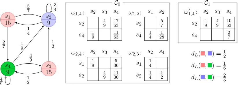
Example 5.1 (On-the-fly computation). Consider the CTMC in Figure 3, and assume we want to compute the λ-discounted bisimilarity distance between statess1 and s4, forλ= 12.
Algorithm 1 starts by guessing an initial coupling structure C0. This is done by con-sidering only the pairs of states which are really needed in the computation. Starting from the pair (s1, s4) a coupling in ω1,4 ∈Ω(τ(s1), τ(s4)) is guessed as in Figure 3 and
s1 15 s2 9 s3 15 s4 9 5 7 2 7 1 4 3 4 1 2 1 2 1 9 4 9 4 9
s2 s3 s4
s2 49 1763
s4 19 1163
ω1,4: s1 s2
s2 57
s4 14 281
ω1,2:
s2 s4
s1 14
s2 14 12
ω2,3:
s2 s3 s4
s1 19 365
s2 49 1136
ω2,4:
C0
s2 s3 s4
s2 19 49 1063
s4 27
ω1′,4:
C1
dL( , ) = 12
dL( , ) = 16
[image:20.612.103.515.117.264.2]dL( , ) = 23
Figure 3: Execution trace for the computation ofδ1
2(1,4) (details in Example 5.1). and the guess of three new couplings ω2,3 ∈ Ω(τ(s2), τ(s3)), ω2,4 ∈ Ω(τ(s2), τ(s4)), and
ω1,2 ∈ Ω(τ(s1), τ(s2)), to be associated in C0 with their corresponding pairs. Since no
other pairs are demanded, the construction of C0 terminates as shown in Figure 3. The
λ-discrepancy associated with C0 for the pair (s1, s4) is obtained as the solution of the
following reduced linear program arg min
d
(d1,4+d2,3+d2,4+d1,2)
d1,4 ≥
1 6
d1,4 ≥
α
2 +
(1−α) 2 ·
4
9 ·d2,3+ 17
63 ·d2,4+ 11 63·
=0
z}|{ d4,4
d2,3 ≥
1 2
d2,3 ≥
α
2 +
(1−α) 2 ·
1
4 ·d1,2+ 1 4 ·
=0
z}|{ d2,2+
1 2 ·d2,4
d2,4 ≥
2 3
d2,4 ≥ 1
2·
1
9 ·d1,2+ 5
36 ·d1,4+ 4
9 ·d2,3+ 11 36 ·d2,4
d1,2 ≥
1 2
d1,2 ≥
α
2 +
(1−α) 2 ·
5
7 ·
=0
z}|{ d2,2 +
1
4·d1,4+ 1 28 ·d2,4
whereα=kexp[15]−exp[9]kTV = 6
√ 3/5
25 (by Equation (2.1)). Note that, the bisimilarity
dis-tance for the pairs (s2, s2) and (s4, s4) is always 0, thusd2,2 andd4,4 are substituted
accord-ingly. The solution of the above linear program isdC0(s
1, s4) = α2 + 5(121−α),dC0(s2, s3) = 12,
dC0(s
2, s4) = 23, anddC0(s1, s2) = 12.
Since, theλ-discrepancy for (s2, s3), (s2, s4), and (s1, s2) equals the distanceLbetween
are removed fromC0. Note that, these pairs will no longer be considered in the construction of a coupling structure.
In order to decrease theλ-discrepancy of (s1, s4), Algorithm 1 constructs a new coupling
structure C1. According to our greedy strategy, C1 is obtained from C0 updating C0(s1, s4)
(i.e., the only coupling left) by the couplingω′1,4∈Ω(τ(s1), τ(s4)) (shown in Figure 3) that is
obtained as the solution of a transportation problem with marginalsτ(s1) andτ(s4), where
the currentλ-discrepancy is taken as cost function. The resulting coupling does not demand for the exploration of new pairs in the CTMC, hence the construction ofC1 terminates. The reduced linear program associated withC1 is given by
arg min d
d1,4
d1,4 ≥
1 6
d1,4 ≥
α
2 +
(1−α) 2 ·
1
9·
=0
z}|{ d2,2 +
4 9 ·
=1 2 z}|{
d2,3 +
10 63 ·
=2 3 z}|{
d2,4 +
2 7 ·
=0
z}|{ d4,4
whose solution is dC1(s
1, s4) =α2 +31(1189−α).
Solving again a new transportation problem with the improved current λ-discrepancy as cost function, we discover that the coupling structure C1 cannot be further improved, hence we stop the computation, returningδλ(s1, s4) =dC1(s1, s4) = α2 +31(1189−α). Remark 5.2. Algorithm 1 can also be used for computing over-approximated distances. Indeed, assuming over-estimates for some particular distances are already known, they can be taken as inputs and used in our algorithm simply storing them in the variable d and treated as “exact” values. In this way our method will return the least over-approximation of the distance agreeing with the given over-estimates. This modification of the algorithm can be used to further decrease the exploration of the CTMC. Moreover, it can be employed in combination with approximated algorithms, having the advantage of an on-the-fly state
space exploration.
6. Experimental Results
In this section, we evaluate the performance of the on-the-fly algorithm on a collection of randomly generated CTMCs7
.
First, we compare the execution times of the on-the-fly algorithm with those of the iterative method proposed in Section 2.1. Since the iterative method only allows for the computation of the distance for all state pairs at once, the comparison is (in fairness) made with respect to runs of our on-the-fly algorithm with input query being the set of all state pairs. For each input instance, the comparison involves the following steps:
(a) we run the on-the-fly algorithm, storing both execution time and the number of solved transportation problems,
(b) then, on the same instance, we execute the iterative method until the running time exceeds that of step 1. We report the number of iterations and the number of solved transportation problems.
7
The tests have been performed on a prototype implementation coded in Wolfram Mathematicar9
# States On-the-Fly (exact) Iterating (approximated) Approx. Time (s) # TPs # Iterations # TPs Error 10 0.352 10.500 2.660 266.667 0.0339 12 0.772 19.700 2.850 410.403 0.0388 14 2.496 35.800 3.880 760.480 0.0318 16 4.549 50.607 5.142 1316.570 0.0230 18 13.709 78.611 6.638 2151.021 0.0206 20 22.044 109.146 7.243 2897.560 0.0149 22 50.258 140.727 7.409 3586.010 0.0145 24 67.049 175.481 7.826 4508.310 0.0141 26 112.924 219.255 9.509 6428.150 0.0025 28 247.583 295.533 11.133 8728.530 0.0004 30 284.252 307.698 10.679 9611.320 0.0006 40 296.633 330.824 11.294 18070.600 0.0004 50 807.522 368.500 16.900 42250.000 0.00001
Table 1: Comparison between the on-the-fly algorithm and the iterative method.
# States out-deg = 3 3≤out-deg≤# States/2 Time (s) # TPs Time (s) # TPs 30 0.304 0.383 18.113 21.379 40 2.045 0.954 34.582 22.877 50 7.832 16.304 50.258 139.427
# States out-deg = 3 Time (s) # TPs 60 34.858 12.053 70 48.016 14.166 80 73.419 29.383 90 75.591 13.116 100 158.027 20.301
Table 2: Average performances of the on-the-fly algorithm on single-pair queries. Execution times and number of performed TPs are reported for CTMCs with different out-degree. For instances with more than 50 states the out-degree is fixed to 3;
(c) Finally, we calculate the approximation error between the exact solution δλ computed by our method at step 1 and the approximate resultdobtained in step 2 by the iterative method, askδλ−dk.
This has been made on a collection of CTMCs varying from 10 to 50 states. For each
n= 10, . . . ,30, we have considered 40 randomly generated CTMCs per out-degree, varying from 3 ton; whereas forn= 40 and 50, the out-degree varies from 3 to 10. Table 1 reports the average results of the comparison obtained for a discount factor λ= 12.
As it can be seen, our use of a greedy strategy in the construction of the couplings leads to a significant improvement in the performances. We are able to compute the exact solution before the iterative method can under-approximate it with an absolute error of
≈0.03, which is a non-negligible error for a value within the interval [0,1].
states of the CTMCs. The results show that, when the out-degree of the CTMCs is low, our algorithm performs orders of magnitude better than in the general case.
Notably, our on-the-fly method scales well when the out-degree is small and successive computation of the currentλ-discrepancy are performed on a relatively small set of pairs.
As for the linear program characterization of the bisimilarity distance illustrated in Section 2.2, tests performed on small CTMCs show that solving Dλ(M) is inefficient in practice, both using the simplex and the interior-point methods8. Even for CTMCs with less than 20 states, the computation times are in the order of hours. For this reason, the efficiency of our on-the-fly technique is by no mean comparable to the linear program solution.
7. Conclusions and Future Work
In this paper, we proposed a bisimilarity pseudometric for measuring the behavioral sim-ilarity between CTMCs, that extends that on MCs introduced by Desharnais et al. in [DGJP04]. Moreover, we gave a novel linear program characterization of the distance that, differently from similar previous proposals, have a number of constraints which is poly-nomial in the size of the CTMC. This proved that the bisimilarity pseudometric can be computed in polynomial time. Finally, we defined an on-the-fly algorithm for computing the bisimilarity distance. We demonstrated that, using on-the-fly techniques the computa-tion time is improved with orders of magnitude with respect to the corresponding iterative and linear program approaches. Moreover, our technique allows for the computation on a set of target distances that might be done by only investigating a significantly reduced set of states, and for further improvement of speed.
Our algorithm can be practically used to address a large spectrum of problems. For instance, it can be seen as a method to decide whether two states of a given CTMC are probabilistic bisimilar, to identify bisimilarity classes, or to solve lumpability problems. It is sufficiently robust to be used with approximation techniques as, for instance, to provide a least over-approximation of the behavioral distance given over-estimates of some particular distances. It can be integrated with other approximate algorithms, having the advantage of the efficient on-the-fly state space exploration.
Having a practically efficient tool to compute bisimilarity distances opens the perspec-tive of new applications already announced in previous research papers. One of these is the state space reduction problem for CTMCs. Our technique can be used in this context as an indicator for the sets of neighbour states that can be collapsed due to their similarity; it also provides a tool to estimate the difference between the initial CTMC and the reduced one, hence a tool for the approximation theory of CTMCs.
Acknowledgement
We would like to thank the anonymous reviewers that with their suggestions greatly im-proved the presentation of the paper. In particular, we thank Franck van Breugel for the helpful discussions and for providing us the omitted proofs in the proceeding publication of [CvBW12].
8The implementation is done in Wolfram Mathematicar9 and uses the Linear Program solvers available