Orbit period modulation for relative motion using continuous low thrust in the two-body and restricted three-body problems

https://doi.org/10.1007/s10569-017-9807-3

O R I G I NA L A RT I C L E

Orbit period modulation for relative motion using

continuous low thrust in the two-body and restricted

three-body problems

C. S. Arnot1 · C. R. McInnes2 ·R. J. McKay1 · M. Macdonald1 · J. Biggs3

Received: 1 February 2017 / Revised: 9 November 2017 / Accepted: 13 November 2017 © The Author(s) 2018. This article is an open access publication

Abstract This paper presents rich new families of relative orbits for spacecraft formation flight generated through the application of continuous thrust with only minimal intervention into the dynamics of the problem. Such simplicity facilitates implementation for small, low-cost spacecraft with only position state feedback, and yet permits interesting and novel relative orbits in both two- and three-body systems with potential future applications in space-based interferometry, hyperspectral sensing, and on-orbit inspection. Position feedback is used to modify the natural frequencies of the linearised relative dynamics through direct manipulation of the system eigenvalues, producing new families of stable relative orbits. Specifically, in the Hill–Clohessy–Wiltshire frame, simple adaptations of the linearised dynamics are used to produce a circular relative orbit, frequency-modulated out-of-plane motion, and a novel doubly periodic cylindrical relative trajectory for the purposes of on-orbit inspection. Within the circular restricted three-body problem, a similar minimal approach with position feedback is used to generate new families of stable, frequency-modulated relative orbits in the vicinity of a Lagrange point, culminating in the derivation of the gain requirements for synchronisation of the in-plane and out-of-plane frequencies to yield a singly periodic tilted elliptical relative

B

callum.arnot@strath.ac.uk C. R. McInnes

colin.mcinnes@glasgow.ac.uk R. J. McKay

robmckay82@gmail.com M. Macdonald

malcolm.macdonald.102@strath.ac.uk J. Biggs

jamesdouglas.biggs@polimi.it

1 _{Advanced Space Concepts Laboratory, Department of Mechanical and Aerospace Engineering,} University of Strathclyde, Glasgow, UK

2 _{School of Engineering, University of Glasgow, Glasgow, UK}

orbit with potential use as a Lunar far-side communications relay. Thevrequirements for the cylindrical relative orbit and singly periodic Lagrange point orbit are analysed, and it is shown that these requirements are modest and feasible for existing low-thrust propulsion technology.

Keywords Non-Keplerian orbits·Continuous low thrust·Relative spacecraft motion· Orbit period modulation·Hill–Clohessy–Wiltshire equations·Restricted three-body problem

1 Introduction

1.1 Forced relative motion

After the advent of spacecraft rendezvous and docking, perhaps one of the earliest recogni-tions of the potential utility of spacecraft formation flight was in the form of a space-based interferometer, proposed by Sholomitsky et al. (1977), and then similarly by Labeyrie (1978). In the latter decades of the twentieth-century, the uses of multi-spacecraft missions were explored further, and indeed in recent years several missions using formation flight have flown, perhaps most prominently the ESA Cluster and NASA Magnetospheric Multiscale (MMS) missions.

The guidance and control of a wide variety of formation-flying concepts have been compre-hensively surveyed in the previous decade, encompassing such applications as hyperspectral sensing and fractionated spacecraft (Scharf et al.2003,2004). Until very recently, such con-cepts generally assumed the use of conventional chemical propulsion for relative motion control. Low specific impulse and high thrust impose limitations on spacecraft formations, since the availablevis low and thrusters offer discrete impulses. Using such propulsion implies that the spacecraft must follow unforced ballistic trajectories between impulses. It has therefore been proposed that the continuous low thrust offered by modern electrostatic thrusters could add versatility to spacecraft formation flight (Austin et al.1977). The thrust magnitudes required for formation keeping are generally small, and so several concepts for efficient electrostatic microthrusters have been developed (Cen and Xu2010; Wirz et al. 2004). Alternatively, Coulomb forces for formation control have been investigated by sev-eral authors (e.g. Natarajan, and Schaub2006; Schaub and Hussein2010; King et al.2003; Schaub et al.2006).

Displacing the plane of an orbit using out-of-plane thrust was explored most prominently by Nock (1984), Yashko and Hastings (1996) and McInnes (1977). These displaced-plane orbits are often referred to as non-Keplerian orbits (NKOs), since the system barycentre is not in the orbit plane. The use of Solar sails to generate non-Keplerian geostationary orbits was considered by Baig and McInnes (2008) and Heiligers et al. (2012). Many authors have also established the existence, stability, and controllability conditions of such orbits (McInnes 1977, 1998; Scheeres1999; Xu and Xu2008; Bombardelli and Pelez2011; Ceriotti et al. 2012; Aliasi et al.2012), and recently McKay et al. performed a broad survey of NKOs and their utility (McKay et al.2011). Recently, Wang et al. offered a new methodology for analysis of the formation flight of electric sails operating in NKOs, and subsequently presented a control framework for such sail formations (Wang et al.2017a,b).

1.2 Problem motivation and approach

In this paper, rich new families of relative trajectories for spacecraft formation flight are generated through the application of continuous thrust. In both the two-body Hill–Clohessy– Wiltshire frame and the circular restricted three-body problem, it is shown that simple position feedback can be used to modify the natural frequencies of the linearised dynamics through direct manipulation of the system eigenvalues and to thereby produce interesting and novel stable relative orbits. Whereas past authors have generally used a top-down engineering approach, designing active controllers with which to force a spacecraft onto a predetermined reference trajectory (e.g. Scheeres et al.2003; Hsiao and Scheeres2005; Bando and Ichikawa 2013), this paper instead seeks to generate rich new families of orbits with only position feedback and without a reference trajectory, thereby only minimally intervening into the dynamics of the problem. The assumption of the use of only position feedback instead of full-state feedback is justified by the goal of providing access to useful new trajectories for small, low-cost spacecraft equipped only with position sensing relative to a target spacecraft (e.g. Sansone et al.2017). The use of only position feedback mitigates the difficulties in implementing accurate relative velocity sensing aboard such a spacecraft and also avoids the need for taking the time derivative of the position (a method which is inherently prone to noise errors), whilst still permitting attainment of relative orbits in both two- and three-body systems with potential future applications in space-based interferometry, hyperspectral sensing, and on-orbit inspection.

In 2010, NASA published a comprehensive study of orbit servicing, concluding that on-orbit servicing infrastructure was an essential and economical supporting step for future space missions (NASA GSFC2010). It follows that on-orbit inspection is a necessary precursor to servicing, since it allows for advance detection and identification of points of failure aboard a satellite. In geostationary orbit, for example, many satellites could be inspected by a single small satellite or formations of small satellites in order to determine the need for servicing. Past authors have therefore proposed a number of free-flying strategies for on-orbit inspection (Woffinden2004), and notably for space situational awareness (Erdner2007) a 15 nanosatellite constellation tasked with inspecting the entire geostationary ring in less than a single year. However, the necessity of ballistic flight imposes limitations on an inspection mission—limitations which can be effectively addressed with the introduction of continuous low thrust.

system. Due to the decoupling of the in-plane motion and out-of-plane motion, it is possi-ble to have the case where the periods are distinct, and to cause the spacecraft to follow, for example, a helix of varying pitch around a target. This new and novel trajectory is a useful ability for on-orbit inspection as it allows for a detailed sweep of a target. Alterna-tively, for astronomy by a disaggregated spacecraft, a lens and formation of sensors could be made to rotate uniformly around a core spacecraft and thereby scan a large swathe of the sky.

The concept of using thrust proportional to relative position only to modify the natural periods of motion can also be usefully applied to the circular restricted three-body problem. Though the problem is normally nonlinear, the motion of a spacecraft in proximity to a Lagrange point can be linearised, and thrust proportional to position can be implemented. This can be used firstly to force the system to become linearly stable, and secondly to modify the natural frequencies of the motion. Further, the in-plane motion and out-of-plane motion can be coupled to yield a singly periodic orbit around the Lagrange point, which could be applied to provide a constantly visible communications relay for another spacecraft.

The structure of the paper is as follows. Section2 builds on initial work (Arnot and McInnes2015) concerning forced motion relative to a circular two-body reference orbit, and using a state-space approach systematically explores a number of different types of forced relative motion, with the final aim of generating a novel doubly periodic cylindrical relative orbit for on-orbit inspection of a target by a chase spacecraft. Section3concerns forced motion relative to a Lagrange point in the restricted three-body problem, using an approach similar to Sect.2and to recent authors such as Bando and Ichikawa (2013) to modify the natural frequencies of motion within regions of closed-loop stability, producing new and interesting types of multiply- and singly periodic relative trajectories. These novel relative orbits have wide ranging applications, such as for hyperspectral astronomy and the provision of constantly visible communications relays.

2 Thrust augmented relative motion in the two-body rotating frame

This section comprises the systematic derivation and exploration of new families of forced relative orbits using linearised dynamics derived from the two-body problem. Using a state-space method, simple position feedback control will be used to manipulate the eigenvalues (and therefore the natural frequencies) of the system to produce interesting and novel new relative orbits. The primary aim of this section is to generate relative orbits with potential future applications in on-orbit inspection—an area where the advantages of modifying the frequencies of periodic motion are readily apparent.

Figure1illustrates a rotating reference frame centred on a circular reference orbit about a point-mass central body. The motion of a chase spacecraft relative to a target on the reference orbit can be described by the linear Hill–Clohessy–Wiltshire (HCW) equations (Wiltshire and Clohessy1960). With the target at the origin of the reference frame, we take thex-axis as following the radius vector from the central mass through the target, thez-axis following the orbital angular momentum vector, and they-axis points in the along-track direction of the target’s motion around the central body. This reference frame forms the environment in which new relative orbits are generated throughout this section of the paper.

Fig. 1 Rotating frame of reference

¨

x =3n2x+2ny˙+ux (1a) ¨

y = −2nx˙+uy (1b)

¨

z= −n2z+uz, (1c)

whereux,uy, anduzare the thrust-induced acceleration terms, andnis the angular velocity of the rotating frame. This is in turn given by

n=

μ/R3 ₍₂₎

in whichμis the gravitational parameter andRis the inertial-frame orbit radius.

To apply controlling thrust terms to the HCW equations, the motion from Eq. (1a–1c) is first converted to the state-space form

˙

x=Ax+Bu, (3)

wherex= [x y z x˙ y˙ z˙]T, and

A=

⎡ ⎢ ⎢ ⎢ ⎢ ⎢ ⎢ ⎣

0 0 0 1 0 0

0 0 0 0 1 0

0 0 0 0 0 1

3n2 _{0 0 0 2n 0}

0 0 0 −2n 0 0

0 0 −n2 0 0 0

⎤ ⎥ ⎥ ⎥ ⎥ ⎥ ⎥ ⎦

(4)

B=

⎡ ⎢ ⎢ ⎢ ⎢ ⎢ ⎢ ⎣

0 0 0

0 0 0

0 0 0

1 0 0

0 1 0

0 0 1

⎤ ⎥ ⎥ ⎥ ⎥ ⎥ ⎥ ⎦

. (5)

An extremely simple strategy is proposed whereby the thrust-induced acceleration is proportional to the displacement in the radial, along-track, and out-of-plane axes only. The acceleration-law is defined by

The feedback gain matrixK is given by

K =

⎡

⎣K011 K022 00 00 00 00

0 0 K33 0 0 0

⎤

⎦_. (7)

The upper bound of the input acceleration can be easily defined therefore in terms of the maximum displacement in each axis, as

umax= ⎡ ⎣|_|uuxymaxmax||

|uzmax| ⎤ ⎦₌

⎡ ⎣KK1122xymaxmax

K33zmax ⎤

⎦_. (8)

The control acceleration can therefore be bounded through the appropriate selection of the maximum displacement in each axis, which is in turn generally determined from the initial conditions.

Now, set Ac = A−B K, which has eigenvaluesλand corresponding eigenvectorsV.

The general eigenvalues are found to be

λ= ⎡ ⎢ ⎢ ⎢ ⎢ ⎢ ⎢ ⎢ ⎢ ⎢ ⎢ ⎢ ⎢ ⎢ ⎢ ⎣ −

−K11−K22−n2₋√_(K11−K22)2_{+2(K11+7K22)n}2_+n4 √

2

−K11−K22−n2₋√_(K11−K

22)2+2(K11+7K22)n2+n4 √

2

−

−K11−K22−n2₊√_(K11−K

22)2+2(K11+7K22)n2+n4 √

2

−K11−K22−n2₊√_(K11−K

22)2+2(K11+7K22)n2+n4 √

2

− −K33−n2

−K33−n2

⎤ ⎥ ⎥ ⎥ ⎥ ⎥ ⎥ ⎥ ⎥ ⎥ ⎥ ⎥ ⎥ ⎥ ⎥ ⎦ . (9)

Since the eigenvalues represent the natural frequencies of the system, modifyingK there-fore directly modifies these frequencies. Feedback gainsK11andK22both affect the first two

conjugate pairs of eigenvalues corresponding to the in-plane motion, andK33only affects a

single decoupled pair of eigenvalues, corresponding to thez-axis motion. This key idea of modifying the natural frequencies of the system through feedback is used to produce interest-ing and novel relative trajectories in both the two-body and subsequent three-body sections of this paper.

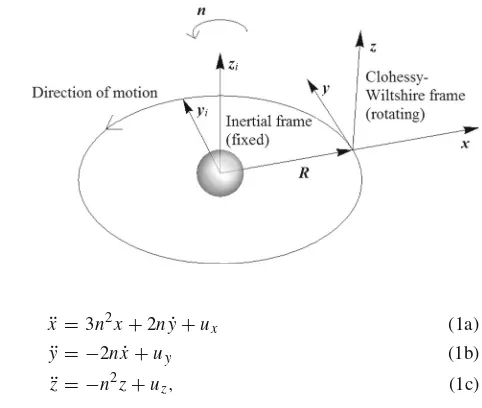
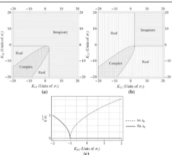
Stable oscillatory behaviour occurs when the eigenvalues are imaginary, so it is useful to find the corresponding range of gains for this behaviour. Considering the second, fourth, and sixth elements of Eq. (9),λ2,λ4, andλ6, since these eigenvalues each form one half of

a conjugate pair, plots indicating the regions in which these eigenvalues are real, complex, and imaginary are given in Fig.2. Unstable regions are found where the real parts of the eigenvalues are greater than zero. The eigenvalueλ6is considered separately since it is only

affected by a single gain,K33.

Fig. 2 Regions for which (a)λ2, (b)λ4, and (c)λ6are purely imaginary, purely real, and complex

Φ=W(t)W−1(0). (10)

The fundamental solution to the system,W(t), can be found using

W(t)=V

⎡ ⎢ ⎢ ⎢ ⎣

eλ1t ₀ · · · ₀

0 eλ2t · · · ₀

... ... ...

0 · · · eλ6t

⎤ ⎥ ⎥ ⎥

⎦. (11)

Note that, in the case where the eigenvalues are complex, it is necessary to take the real and imaginary parts of the complex solution separately to find the real fundamental solution to the system,Wr(t). The general solution to the system, including control inputs, can then

be found using

x(t)=Wr(t)Wr−1(0)x(0)+Wr(t)

t

t0

Wr−1(τ)Budτ. (12)

In the case thatK11=K22=K33=0, the time domain solution to the system is equal

⎡ ⎢ ⎢ ⎢ ⎢ ⎢ ⎢ ⎣

x(t) y(t) z(t) ˙ x(t)

˙ y(t) ˙ z(t)

⎤ ⎥ ⎥ ⎥ ⎥ ⎥ ⎥ ⎦ = ⎡ ⎢ ⎢ ⎢ ⎢ ⎢ ⎢ ⎣

4−3 cosnt 0 0 1_nsinnt _n2(1−cosnt) 0 6(sinnt−nt) 1 0 −2_n(1−cosnt) 1_n(4 sinnt−3nt) 0

0 0 cosnt 0 0 _n1sinnt

3nsinnt 0 0 cosnt 2 sinnt 0

−6(1−cosnt) 0 0 −2 sinnt 4 cosnt−3 0

0 0 −nsinnt 0 0 cosnt

⎤ ⎥ ⎥ ⎥ ⎥ ⎥ ⎥ ⎦ ⎡ ⎢ ⎢ ⎢ ⎢ ⎢ ⎢ ⎣ x0 y0 z0 ˙ x0 ˙ y0 ˙ z0 ⎤ ⎥ ⎥ ⎥ ⎥ ⎥ ⎥ ⎦ . (13)

Since the aim of this work is to modify the natural frequencies of the system and thereby generate novel trajectories, it is necessary that at least one of the gains is nonzero, and so the solution in Eq. (13) cannot be used in its entirety. However, part of this solution will be used in certainvcalculations later in this section.

2.1 Artificial equilibria and a simple circular relative orbit

A simple yet interesting case to demonstrate the eigenvalue-based approach is that of the generation of artificial static equilibria in the rotating frame using continuous thrust, since, if nonzero initial velocity isnotassumed, it is useful to characterise the type and frequency of motion followed by the spacecraft. Such equilibria in the rotating frame are equivalent to type III non-Keplerian orbits when viewed from an inertial frame (McInnes1977).

Consider the state vectorx = [x,y,z,x˙,y˙,z˙]T in which x˙,y˙, andz˙must be zero for a static displacement. Sinceu= −K x, the system state equation isx˙ = Ax+B(−K x). With zero initial velocity (x˙0 = ˙y0 = ˙z0 =0) the system state is held constant by selecting

the feedback gains as

K =

⎡ ⎣3n

2 _{0 0 0 0 0}

0 0 0 0 0 0

0 0 −n2 _{0 0 0}

⎤

⎦. (14)

With reference to Fig.2, the motion should be stable, with all nonzero eigenvalues being imaginary. Indeed, the eigenvalues of the system are found to be

λ= ⎡ ⎢ ⎢ ⎢ ⎢ ⎢ ⎢ ⎣

−2i n

2i n

0 0 0 0 ⎤ ⎥ ⎥ ⎥ ⎥ ⎥ ⎥ ⎦ . (15)

If the initial velocity is zero, there are no oscillations and the spacecraft remains fixed at its initial position. However, with nonzero initial velocity, since the coefficient of bothλ1

andλ2is 2, the forced natural frequency of the motion in thex–yplane is twice the unforced

natural frequency. SinceK22=0, for static formations in the rotating frame, the along-track

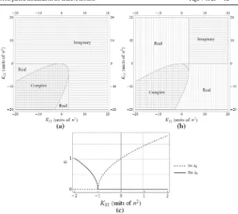
position is arbitrary as it does not affect the required thrust. For a thrust-induced acceleration vectoruof fixed magnitude, a required thrust vector field for static equilibrium positions in thex–zplane can be generated, as shown in Fig.3where all values are normalised by the reference orbit radius. All subsequent plots of relative orbits in the two-body section are also normalised in this way.

Fig. 3 Required thrust vector field for static formations in the

x-zplane, where the position is normalised by the reference orbit radius, and the acceleration is normalised by the reference orbit radius and orbit period

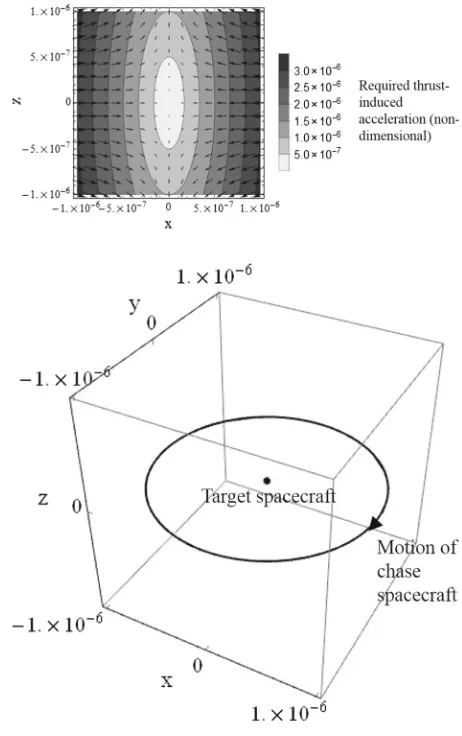
Fig. 4 Non-dimensional in-plane circular relative orbit achieved with single axis thrust

only to add the conditionx˙0 = 2ny0, and with the feedback gains of Eq. (14) the result is

a circular trajectory in thex–yplane. As already indicated, the relative orbit period is half of the reference orbit period. Furthermore, in this case the gainK33is arbitrary because the z-axis motion is decoupled and the circular trajectory exists only in thex–yplane, and so the circular relative orbit is achieved using thrust in only the radial direction. An example of this type of relative motion is plotted in Fig.4.

In the case of zero initial velocity, i.e. for a static formation, theVrequired to maintain the formation is simple to calculate. Since with zero initial velocityux is constant, and assuming independent body-mounted thrusters on each axis, it is possible to use

vx =3n2xτ, (16)

whereτ is the duration for which the formation is maintained. Similarly, sinceuz is also constant, we can use

Using an example of a geostationary target, with Eqs. (16) and (17), theVaccumulated for a chase spacecraft positioned for one sidereal day in a 100 mz-axis statically displaced NKO is 0.046 m s−1_{, and for a 100 mx-axis displacement is 0.138 m s}−1_{. Assuming the use}

of electrostatic ion thrusters with a specific impulse of 3000 s, for a nanosatellite with initial mass of 10 kg, this amounts to a propellant expenditure of only 1.56×10−5and 4.69×10−5 kg, respectively.

2.2 Modulation of the out-of-plane period

Having considered the in-plane behaviour of the system under the feedback gains of Eq. (14), the out-of-plane motion is now considered. WhenK33 = −n2 with some nonzeroz0, the

chase spacecraft is fixed in a displaced non-Keplerian orbit whose plane does not contain the two-body centre of mass. Oppositely, whenK33 = 0, we have the ballistic case, and

the spacecraft oscillates along thez-axis with a period equal to the reference orbit period. A

z-displaced static formation can therefore be considered a periodic relative orbit with infinite out-of-plane period. As noted by Arnot and McInnes (2015), it is possible to modify the period of the periodicz-axis motion by making thez-axis thrust proportional to displacement. The period of the motion along thez-axis is now modified by changing the out-of-plane thrust component.

To begin, it is necessary to substituteK33= −n2withK33= −ψ2, so that the eigenvalue

corresponding to the out-of-plane motion,λ6in Eq. (9), becomes

λ6=

ψ2_−n2_{. (18)}

It follows that

Ac=

⎡ ⎢ ⎢ ⎢ ⎢ ⎢ ⎢ ⎣

0 0 0 1 0 0

0 0 0 0 1 0

0 0 0 0 0 1

−K11+3n2 0 0 0 2n 0

0 −K22 0 −2n 0 0

0 0 ψ2−n2 0 0 0

⎤ ⎥ ⎥ ⎥ ⎥ ⎥ ⎥ ⎦

. (19)

The augmented angular frequency,Ω, is defined by

Ω2_=(n2_−ψ2_{) (20)}

and by

Ω= n

k (21)

in whichkrepresents the number of reference orbit periods in which the thrust augmented relative motion completes a single out-of-plane cycle. Therefore,kcan be considered the augmented period coefficient, so that the period of thez-axis motion isTz =kT. Through use of out-of-plane thrust, the period of thez-axis motion can now be freely chosen.

Substituting Eq. (21) into (20), it is possible to rearrange forψsuch that

ψ=n

1−

₁ k2

. (22)

It can then be shown that the equation of out-of-plane motion is given by

¨

z= −n 2_z

Fig. 5 Relative orbit with forced out-of-plane period of 3T

which is a harmonic oscillator whose natural frequency can now be selected through the coefficient of the out-of-plane thrust law. The maximum input acceleration for this type of relative orbit is given simply by|uzmax| =ψ2z0, assuming that the initial velocity is zero.

An example of thrust augmentedz-axis motion is shown in Fig.5, wherek = 3,x0 = z0=0.5, andy˙0= −2nx0, simulated for three reference orbit periods.

Clearly, whenk = 1, the thrust-induced acceleration in thez-direction is zero, corre-sponding to ballistic motion. However, whenk<1, the thrust is nonzero and in the opposite direction to the casek > 1. In addition, the frequency of oscillation in thez-direction is greater than the unforced frequency. Whenk → ∞, the expression for the thrust accelera-tion simplifies touz=n2z, soK33= −n2, and thez-axis displacement becomes fixed: that

is, the trajectory is equivalent to static equilibria in the rotating frame.

To calculate thevrequired to maintain this type of continuously forced orbit, we must first consider the third row of Eq. (13) which describes the unforced out-of-plane position of the chase spacecraft. Sincez˙0 =0 and the frequency of the out-of-plane motion is now

defined byΩ, the out-of-plane displacement simplifies to

z(t)=z0cosΩt. (24)

It follows that the thrust command,uz, becomes

uz =ψ2z0cosΩt. (25)

|uz| =

ψ2_z

0cosΩt if cosΩt≥0

−ψ2_z

0cosΩt if cosΩt<0

. (26)

The integral then takes the form (Arnot and McInnes2015)

v=ψ2_z 0

η

t=Tz

t=0

|cosΩt|dt+

t=ε+ηTz

t=ηTz

|cosΩt|dt

, (27)

whereηis the integer number of completez-axis motion periods which have elapsed andεis the additional time over the integer number of periods. Thus, the expression for accumulated vbecomes

v=ψ2_z 0

4η

Ω +

t=ε+Tz

t=ηTz

|cosΩt|dt

. (28)

Equation (28) can be integrated for all positive integer values ofη, and for 0≤ε <Tz.

2.3 The cylindrical relative orbit

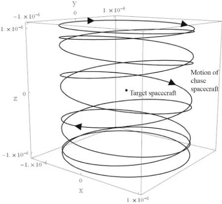
Now that a means to modulate the frequency of the out-of-plane motion is possessed, an interesting and novel application can be envisaged: on-orbit inspection of a target by a chase spacecraft using continuous thrust to modify its relative orbit period. The concept of on-orbit inspection has been explored by other authors; however, the use of continuous low thrust has generally not been considered in this context. Using continuous thrust, a chase space-craft on an inspection mission can actively force its relative motion to enable operationally advantageous new Keplerian and non-Keplerian inspection trajectories. Perhaps the most commercially viable example is that of a small spacecraft tasked to inspect multiple satellites on the geostationary ring, and so previous work has considered the use of a thrust augmented relative orbit in which the chase spacecraft tracks the Sun vector around a target in geo-stationary orbit (Arnot and McInnes2015). Such a trajectory makes use of constant-angle sunlight to facilitate visual inspection. Here the more general case of a cylindrical relative orbit is considered, which makes use of thrust augmented in-plane motion and out-of-plane motion to produce an orbit with two distinct modified periods.

A simple cylindrical relative orbit can be achieved by using the circular in-plane orbit already described (usingK11=3n2andK22=0) combined with out-of-plane orbit period

modulation (K33= −ψ2). Selecting an appropriate out-of-plane period, the result is that the

chase spacecraft performs a helical sweep around the target as it oscillates betweenz0and

−z0with an in-plane period of 0.5T. However, although it is possible to freely select the

out-of-plane period, this type of trajectory has a fixed in-plane period. A circular relative orbit whose period and orientation can also be freely selected would be of greater operational advantage. Bando and Ichikawa (2013) showed that circular and elliptical relative orbits of arbitrary frequency were achievable using active control; however, a useful analytical description of such a family of orbits has apparently not been presented in the literature and is derived parametrically as follows.

To produce a circular trajectory about the target spacecraft, consider first a three-dimensional circle described parametrically by the vector α = [α1, α2, α3]T, which is

collinear with the circle’s transformedx-axis (transformed from thex-axis of the rotating frame and fixed with respect to the circle), and the vector β = [β1, β2, β3]T, which is

radius vector of the circle, andθis the angle between the radius vector and thex-axis as mea-sured in the anticlockwise direction about the circle’s central axis. It is taken thatθ = −γnt

(negative because the motion of the chase spacecraft in thex-y-plane is clockwise), whereγ is the ratio of the target spacecraft’s Keplerian orbit period to that of the circular relative orbit in the rotating frame (for instance, ifγ =1, the period of the circular motion is equal to that of the Keplerian orbit of the target spacecraft), and wherenandthave their usual meaning. The inclusion ofγ permits the modification of the period of the relative orbit, so that

r=c+rcos(θ)α+rsin(θ)β. (29)

The first and second derivatives of Eq. (29) are found to be

˙

r=rγnsin(θ)α−rγncos(θ)β (30)

¨

r= −r(γn)2cos(θ)α−r(γn)2sin(θ)β. (31) It follows that, in this case,x˙= [r˙,r¨]T. Then, referring to Eq. (3), we recall the acceler-ation inputu= [ux,uy,uz]T. Thus, it can be shown that

˙ x= ⎡ ⎢ ⎢ ⎢ ⎢ ⎢ ⎢ ⎣ ˙ x ˙ y ˙ z

3n2x+2ny˙+ux −2nx˙+uy

−n2z+uz

⎤ ⎥ ⎥ ⎥ ⎥ ⎥ ⎥ ⎦ = ⎡ ⎢ ⎢ ⎢ ⎢ ⎢ ⎢ ⎣

rγnsin(θ)α1−rγncos(θ)β1 rγnsin(θ)α2−rγncos(θ)β2 rγnsin(θ)α3−rγncos(θ)β4

−r(γn)2cos(θ)α1−r(γn)2sin(θ)β1

−r(γn)2cos(θ)α2−r(γn)2sin(θ)β2

−r(γn)2cos(θ)α3−r(γn)2sin(θ)β3 ⎤ ⎥ ⎥ ⎥ ⎥ ⎥ ⎥ ⎦ . (32)

The input accelerationucan then be obtained as

u=

⎡ ⎣n

2_(−r(α

1(γ2+3)−2β2γ )cosγnt+r(2α2γ+β1(γ2+3))sinγnt−3c1

−n2rγ ((2α1−β2γ )sinγnt+(α2γ+2β1)cosγnt) n2(−α3r(γ2−1)cosγnt+β3r(γ2−1)sinγnt+c3

⎤ ⎦_.

(33) Usinguxfrom Eq. (33), it can be shown that the single axis thrust case described earlier is a special case of the general thrust equations. Since the special case is a circle in thex-yplane and centred at the origin,α= [1,0,0]T,β = [0,1,0]T, andc= [0,0,0]T,usimplifies to

u=

⎡ ⎣−n

2_r(γ2_{−2γ +3)cosγnt}

−n2rγ (2−γ )sinγnt

0

⎤

⎦, (34)

wherercosγnt ≡ x. Therefore, in order for the first row of Eq. (34) to be equivalent to

ux = −3n2x, it is clear thatγ =2. Interestingly, we note that withγ =2, it follows that

uy =0 and as required,ux = −3n2rcos 2nt ≡ −3n2x, which is equivalent to the earlier state feedback case whereK11=3n2. This provides a particularly simple steering law with

a useful application. The value ofγ also correctly indicates that the period of the in-plane motion is 0.5T. From Eq. (34), it is deduced that the maximum input acceleration in each axis is given by|uxmax| = −n2r(γ2−2γ+3)and|uymax| = −n2rγ (2−γ )for thex-axis

andy-axis, respectively.

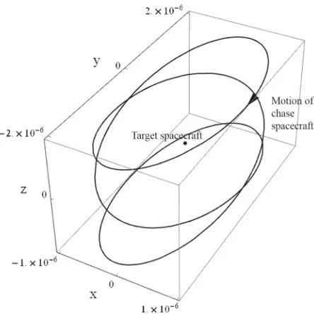
Fig. 6 Cylindrical relative orbit withγ=1 andk=9

natural frequencies of the circular in-plane motion and oscillatory out-of-plane motion can be freely modified. As before, thez-axis position varies sinusoidally between the maximum and minimum displacement. An example cylindrical relative orbit achieved using this approach is displayed in Fig.6, with non-dimensional axes.

Thevrequired to maintain the cylindrical orbit is found by integrating the three thrust acceleration components and summing the result, assuming independent body-mounted thrusters. Taking thexandycomponents from Eq. (34), the moduli are

|ux| =

| −n2r(γ2−2γ +3)|cosγntif cosγnt≥0

−n2_r(γ2_{−2γ+3)cosγntif cosγnt<0} (35a)

|uy| =

| −n2_{rγ (2−γ )|sinγntif sinγnt≥0}

−n2rγ (2−γ )sinγntif sinγnt<0. (35b)

The integrals then become (Arnot and McInnes2015)

vx = | −n2r(γ2−2γ +3)|

q t=Tx y

t=0

|cosγnt|dt+

t=υ+q Tx y

t=q Tx y

|cosγnt|dt

(36a)

vy = | −n2rγ (2−γ )|

q

t=Tx y

t=0

|sinγnt|dt+

t=υ+q Tx y

t=q Tx y

|sinγnt|dt

, (36b)

wherevxandvyare the components ofvin thex- andy-directions, respectively,Tx y is the period of thex-yplanar motion,qis the integer number ofx-yplanar motion periods which have elapsed, andυ is the additional time over the integer number of x-ymotion periods. Integrating, the expressions forvbecome

vx = | −n2r(γ2−2γ +3)|

4q

γn+

t=υ+q Tx y

t=q Tx y

|cosγnt|dt

Fig. 7 Schematic of the circular restricted three-body problem withρ=0.01213 (equivalent to the Earth–Moon system)

vy = | −n2rγ (2−γ )|

4q

γn +

t=υ+q Tx y

t=q Tx y

|sinγnt|dt

. (37b)

Thez-axis component ofvis as given in Eq. (28). Equations (37a) and (37b) can be integrated for all positive integer values ofq, and for 0≤υ <Tx y. Using the Sun vector tracking orbit (which orbits a geostationary target with an in-plane period of one Solar day and out-of-plane period of one year) as an example of this type of orbit (Arnot and McInnes2015), with a 100-m in-plane radius, 43.3 m maximum out-of-plane displacement, and independent axis-aligned thrusters, the totalvfor a full year of operation would be 36.7 m s−1. This would amount to 0.0125 kg of propellant for a 10 kg nanosatellite equipped with electrostatic thrusters with specific impulse of 3000 s.

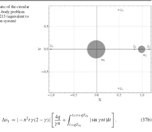
3 Thrust augmented orbits at Lagrange points

Thus far, this paper has considered only relative motion around a circular reference orbit using linearised dynamics derived from the two-body problem. However, a similar approach can be used for the generation of thrust augmented relative orbits in the vicinity of a Lagrange point, in the circular restricted three-body problem (CRTBP), using linearised dynamics for spacecraft relative motion. Whereas the previous section considered the generation of orbits with potential applications for on-orbit inspection, this section aims to derive the feedback gains necessary to synchronise the in-plane and out-of-plane frequencies to produce a stable, three-dimensional, singly periodic orbit with potential utility as an Earth–MoonL2

communications relay with constant visibility from the Earth. A special case of this kind of orbit, controlled using solar radiation pressure, was investigated by Tanaka and Kawaguchi (2016) and can further be considered an extension of Farquhar’s original concept for a Lunar far-side communications relay (Farquhar1968).

time ist. The usual origin of the system is at the barycentre of the two primary masses, the axisXis aligned with the vector connecting the two primary masses (m1andm2) andY is

perpendicular to it such that theX-Yplane is the Earth–Moon plane. However, since the aim is to examine the motion of a low-thrust spacecraft relative to a Lagrange point, it is useful to place the origin of the system at the Lagrange point in question,Li. Using this new origin,

x is aligned with the X-axis,y is aligned with theY-axis, andzcompletes the right-hand coordinate system. The linearised equations of relative motion in the vicinity of the Lagrange point are given by Farquhar (1968)

¨

x =2y˙+(2σi+1)x (38a)

¨

y=(1−σi)y−2x˙ (38b)

¨

z= −σiz. (38c)

It is taken that

σi = ρ

|li(ρ)−1+ρ|3 +

(1−ρ) |li(ρ)+ρ|3

(39)

in whichli(ρ)is the distance of the collinear Lagrange point from the system barycentre. The mass ratioρis given by

ρ= m2

m1+m2.

(40)

The distance of the Lagrange point from the system barycentre can be found by solving the quintic expression resulting from

li(ρ)= 1−ρ

r3 1

(li(ρ)+ρ)+ ρ r3 2

(li(ρ)−1+ρ). (41)

The general state-space form has the same construction as Eq. (3), where x =

[x y z x˙ y˙ z˙]T,uhas the same form as Eq. (6), and K is the same as Eq. (7). The sys-tem matrixAhas the new form

A= ⎡ ⎢ ⎢ ⎢ ⎢ ⎢ ⎢ ⎣

0 0 0 1 0 0

0 0 0 0 1 0

0 0 0 0 0 1

2σi+1 0 0 0 2 0

0 1−σi 0 −2 0 0

0 0 −σi 0 0 0

⎤ ⎥ ⎥ ⎥ ⎥ ⎥ ⎥ ⎦ (42)

andBis the same as Eq. (5). Using the relationAc= A−B Kwhich has eigenvaluesλand

eigenvectorsV, the general eigenvalues of the closed-loop system are found to be

λ= ⎡ ⎢ ⎢ ⎢ ⎢ ⎢ ⎢ ⎢ ⎢ ⎢ ⎢ ⎢ ⎢ ⎢ ⎢ ⎢ ⎢ ⎣ −

−2−K11−K22+σi−

K₁₁2+8(K22−σi)−2K11(−4+K22+3σi)+(K22+3σi)2

√

2

−2−K11−K22+σi−

K2

11+8(K22−σi)−2K11(−4+K22+3σi)+(K22+3σi)2

√

2

−

−2−K11−K22+σi+

K₁₁2+8(K22−σi)−2K11(−4+K22+3σi)+(K22+3σi)2

√

2

−2−K11−K22+σi+

K2

11+8(K22−σi)−2K11(−4+K22+3σi)+(K22+3σi)2

√

2

−_√√−K33−σi

−K33−σi

Fig. 8 Regions for which (a)λ2, (b)λ4, and (c)λ6are purely imaginary, purely real, and complex, for Earth–MoonL2point(σ2=3.19097)

Thus, in similar fashion to the linearised two-body problem, it is possible to modify the natural frequencies of the in-plane motion and out-of-plane motion independently by modifying K. For the Earth–Moon L2 point (ρ = 0.01213,σ2 = 3.19097) the regions

where the eigenvalues are purely imaginary, real, or complex are shown in Fig.8. These regions are similar to those of the two-body system, however unlike the two-body case the region boundaries are dependent onσiand so the stable region changes at different Lagrange points and with differentρ.

With reference to Fig.8, it is worth noting that, unlike within the two-body HCW system, the in-plane motion around the Earth–MoonL2 is naturally unstable. WithK11and K22

both at zero,λ4is positive and real. Therefore, in order to design useful, stable, oscillatory

relative trajectories around the Lagrange point, it is necessary to apply feedback gains such that the eigenvalues become purely imaginary. For the Earth–MoonL2 point, the relative

in-plane motion will be stable and oscillatory when gains of approximatelyK11>2.28σ2

andK22>−0.65σ2are selected.

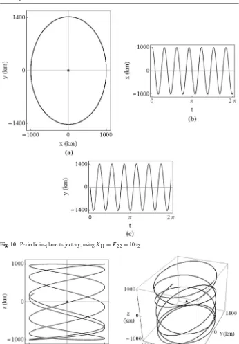
For arbitrary initial conditions, withK11andK22in the stable region, interesting doubly

periodic trajectories are produced. An example of this is shown in Fig.9, where K11 = K22 =10σ2and the initial velocity is zero. Since thez-axis motion is decoupled, it is not

Fig. 9 In-plane trajectory for the doubly periodic case, usingK11 = K22 = 10σ2, for Earth–MoonL2 (σ2=3.19097)

Let p_j +iq_j be the eigenvector corresponding to eigenvalueλj, and consider only the two in-plane eigenvaluesλ2andλ4(since the out-of-plane motion is decoupled) such that j=(2,4). Recalling that the eigenvalueλjis equivalent to the natural frequencyωj, it can be shown that the three-dimensional periodic solution is found from Baig (2009)

⎡ ⎢ ⎢ ⎣ x y ˙ x ˙ y ⎤ ⎥ ⎥

⎦=cos(ω2t)[Ap2+Bq2] +sin(ω2t)[Bp2−Aq2]

+cos(ω4t)[Cp4+Dq4] +sin(ω4t)[Dp4−Cq4]. (44)

From this, by settingt=0, the initial conditions are

⎡ ⎢ ⎢ ⎣ x0 y0 ˙ x0 ˙ y0 ⎤ ⎥ ⎥ ⎦= ⎡ ⎢ ⎢ ⎣

−2ω2B−2ω4D A(h+ω2

2)+C(h+ω42)

2ω2

2A+2ω42C

ω2(h+ω22)B+ω4(h+ω24)D ⎤ ⎥ ⎥

⎦. (45)

The constantsA,B,C, andDare then

⎡ ⎢ ⎢ ⎣ A B C D ⎤ ⎥ ⎥ ⎦= ⎡ ⎢ ⎢ ⎢ ⎢ ⎢ ⎢ ⎢ ⎣

−−hx˙0− ˙x0ω24+2y0ω24

2h(ω2₂−ω2₄) −−2y˙0−hx0−x0ω42

2ω2(ω22−ω24)

−−hx˙0− ˙x0ω22+2y0ω22

2h(ω2₄−ω2₂) −−2y˙0−hx0−x0ω22

2ω4(ω24−ω22)

The initial conditions required forC=0 andD=0 are then found to be

˙

x0

˙

y0

=

⎡ ⎣

2y0ω22 h+ω2 2 −x0(h+ω22)

2 ⎤

⎦_. (47)

So a periodic solution with the same form as the ballistic periodic solution (Baig2009) and dependence on a single natural frequencyω2is found as

x(t)= −Axcos(ω2t+φ) (48a)

y(t)=k Axsin(ω2t+φ) (48b)

in whichk = (ω₂22+_ωh)

2 ,Ax is the amplitude of thex-axis motion, andφis the phase angle. BothK11andK22can now be varied to change the natural frequency andy-axis amplitude

of the elliptical relative orbit around the Lagrange point. The out-of-plane motion, which is always periodic, has the solution

z(t)=Azsin(ω6t+φz), (49)

whereAz is thez-axis amplitude,φz is the phase angle, andω6 is the out-of-plane natural

frequency which can be modified by changingK33. The periodic in-plane motion generated

by these initial conditions is shown in Fig.10, whereK11 = K22 = 10σ2 and the initial

velocity is as in Eq. (47).

It can then be shown that 3-D periodic orbits are achieved whenω2/ω6is a rational number,

and quasi-periodic Lissajous trajectories are attained whenω2/ω6is irrational. An example

of a thrust augmented Lissajous trajectory is plotted in Fig.11, whereK11= K22 =10σ2

andK33=0.

Forω2=ω6, it is necessary that

K33=

2+K11+K22−3σi+

K2

11+8(K22−σi)−2K11(−4+K22+3σi)+(K22+3σi)2

2 .

(50)

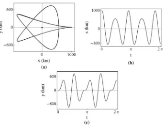
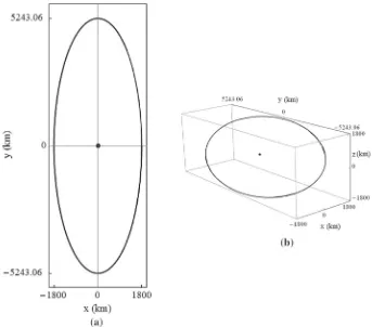
This produces a tilted periodic orbit with a potential application in providing anL2

com-munications relay for the far side of the Moon with respect to the Earth, as an extension of the concept first proposed by Farquhar (1968): instead of out-of-plane phase-jump control impulses, continuous low thrust with gain governed by Eq. (50) is used to prevent occultation of the spacecraft behind the Moon. Constant line of sight with Earth is achieved by ensuring thatAxandAzare greater than the radius of the Moon’s relative umbra. The in-plane and 3-D trajectories of a spacecraft on such an orbit around the Earth–MoonL2are shown in Fig.12,

forAx=Az=1800 km. For this example orbit, with zero thrust in the in-plane directions, the peak thrust-induced acceleration in thez-axis is 3.56µm s−2. The requiredvzfor one year of operation is 74.4 m s−1_{, corresponding to a 0.025 kg propellant expenditure for a}

spacecraft with initial mass of 10 kg, equipped with electrostatic thrusters ofIsp=3000 s.

4 Conclusions

Fig. 10 Periodic in-plane trajectory, usingK11=K22=10σ2

Fig. 12 Trajectory around Earth–MoonL2point whenωx y=ωz, usingK11=K22=0

stable relative orbits in both the two-body and restricted three-body problems, whilst requir-ing only minimal intervention into the dynamics of the problem, to permit implementation aboard small, low-cost spacecraft. One main contribution of this paper is the parametric derivation of a forced circular orbit of arbitrary dimension, orientation, and period rela-tive to a target on a circular two-body orbit. A second contribution is the derivation of thrust commands for out-of-plane period modulation, leading to the analytical description of a cylindrical relative orbit in the two-body rotating frame, with potential future appli-cations in on-orbit inspection. A third contribution is the derivation of gain requirements for the synchronisation of in-plane and out-of-plane periods of a relative orbit around a Lagrange point in the restricted three-body problem, such that a stable, singly periodic 3-D trajectory can be accessed for the purposes of providing a constantly visible Earth– Moon L2 communications relay. Further, the propellant requirements for each new orbit

type are relatively small and achievable when the use of modern electrostatic thrusters is assumed.

Open Access This article is distributed under the terms of the Creative Commons Attribution 4.0 Interna-tional License (http://creativecommons.org/licenses/by/4.0/), which permits unrestricted use, distribution, and reproduction in any medium, provided you give appropriate credit to the original author(s) and the source, provide a link to the Creative Commons license, and indicate if changes were made.

References

Aliasi, G., Mengali, G., Quarta, A.A.: Artificial equilibrium points for a generalized sail in the elliptic restricted three-body problem. Celest. Mech. Dyn. Astron.114(1–2), 181–200 (2012).https://doi.org/10.1007/ s10569-012-9425-z

Arnot, C.S., McInnes, C.R.: Low thrust augmented spacecraft formation-flying for on-orbit inspection. In: 66th International Astronautical Congress, IAC-15-C1.8.1.x28589 (2015)

Austin, R.E., Dod, R.E., Terwilliger, C.H.: The ubiquitous solar electric propulsion stage. Acta Astronaut.

4(5–6), 671–694 (1977)

Baig, S.: Non-Keplerian orbits for low-thrust propulsion, Ph.D. thesis, Department of Mechanical Engineering, University of Strathclyde (2009)

Baig, S., McInnes, C.R.: Artificial three-body equilibria for hybrid low-thrust propulsion. J. Guid. Control Dyn.31(2), 1644–1655 (2008)

Bando, M., Ichikawa, A.: Formation flying near the libration points in the elliptic restricted three-body problem. In: 5th International Conference on Spacecraft Formation Flying Missions and Trajectories, Munich, Germany (2013)

Bando, M., Ichikawa, A.: Active formation flying along an elliptic orbit. J. Guid. Control Dyn. (2013).https:// doi.org/10.2514/1.57703

Bombardelli, C., Pelez, J.: On the stability of artificial equilibrium points in the circular restricted three-body problem. Celest. Mech. Dyn. Astron.109(1), 13–26 (2011). https://doi.org/10.1007/s10569-010-9317-z

Cen, J.W., Xu, J.L.: Performance evaluation and flow visualization of a MEMS based vaporizing liquid micro-thruster. Acta Astronaut.67(3–4), 468–482 (2010)

Ceriotti, M., McInnes, C.R.: Natural and sail-displaced doubly-symmetric Lagrange point orbits for polar coverage. Celest. Mech. Dyn. Astron.114(1–2), 151–180 (2012). https://doi.org/10.1007/s10569-012-9422-2

Cielaszyk, D., Wie, B.: New approach to halo orbit determination and control. J. Guid. Control Dyn.19(2), 266–273 (1996)

Dusek, H.M.: Motion in the vicinity of libration points of a generalized restricted three-body model. Prog. Astronaut. Aeronaut.17, 37–54 (1966)

Erdner, M.T.: Smaller satellite operations near geostationary orbit, M.Sc. thesis, Naval Postgraduate School, Monterey, CA (2007)

Farquhar, R.W.: The Control and Use of Libration-Point Satellites, Ph.D. thesis, Department of Aeronautics and Astronautics, Stanford University, Stanford, California (1968)

Heiligers, J., McInnes, C.R., Biggs, J.D., Ceriotti, M.: Displaced geostationary orbits using hybrid low-thrust propulsion. Acta Astron.71, 51–67 (2012).https://doi.org/10.1016/j.actaastro.2011.08.012

Hsiao, F.Y., Scheeres, D.J.: Design of spacecraft formation orbits relative to a stabilized trajectory. J. Guid. Control Dyn.28(4), 782–794 (2005)

King, L.B., Parker, G.G., Deshmukh, S., Chong, J.-H.: Study of interspacecraft Coulomb forces and implica-tions for formation flying. J. Propuls. Power19(3), 497–505 (2003).https://doi.org/10.2514/2.6133

Labeyrie, A.: Stellar interferometry methods. Ann. Rev. Astron. Astrophys.16(1), 77–102 (1978)

McInnes, C.R.: The existence and stability of families of displaced two-body orbits. Celest. Mech. Dyn. Astron.

67(2), 167–180 (1997).https://doi.org/10.1023/A:1008280609889

McInnes, C.R.: Dynamics, stability, and control of displaced non-Keplerian orbits. J. Guid. Control Dyn.

21(5), 799–805 (1998).https://doi.org/10.2514/2.4309

McKay, R.J., Macdonald, M., Biggs, J., McInnes, C.R.: Survey of highly non-Keplerian orbits with low-thrust propulsion. J. Guid. Control Dyn.34(3), 645–666 (2011).https://doi.org/10.2514/1.52133

Morimoto, M.Y., Yamakawa, H., Uesugi, K.: Artificial equilibrium points in the low-thrust restricted three-body problem. J. Guid. Control Dyn. (2007).https://doi.org/10.2514/1.26771

NASA GSFC.: On-Orbit Satellite Servicing Study Project Report, NASA Project Report NP-2010-08-162-GSFC, Greenbelt, MD (2010)

Nock, K.T.: Rendezvous with Saturns Rings, Planetary Rings: 1st International Meeting, pp. 743–759. CNES, Toulouse (1984)

Sansone, F., Branz, F., Francesconi, A.: A Relative Navigation Sensor for Cubesats Based on Retro-Reflective Markers, 2017 IEEE International Workshop on Metrology for AeroSpace. IEEE, Padua (2017) Scharf, D.P., Hadaegh, F.Y., Ploen, S.R.: A survey of spacecraft formation flying guidance and control (part

I): guidance. In: Proceedings of the 2003 American Control Conference, vol. 2, pp. 1733–1739. Denver, Colorado (2003).https://doi.org/10.1109/ACC.2003.1239845

Scharf, D.P., Hadaegh, F.Y., Ploen, S.R.: A survey of spacecraft formation flying guidance and control (part II): control. In: Proceedings of the 2004 American Control Conference, vol. 4, pp. 2976–2985. Boston, Massachusetts (2004)

Schaub, H., Hussein, I.I.: Stability and reconfiguration analysis of a circularly spinning two-craft Coulomb tether. IEEE Trans. Aerosp. Electron. Syst.46(4), 1675–1686 (2010).https://doi.org/10.1109/AERO. 2007.352670

Schaub, H., Hall, C.D., Berryman, J.: Necessary conditions for circularly-restricted static Coulomb formations. J. Astronaut. Sci54(3), 525–541 (2006).https://doi.org/10.1007/BF03256504

Scheeres, D.J.: Stability of hovering orbits around small bodies. Adv. Astron. Sci.102, 855–866 (1999) Scheeres, D.J., Hsiao, F.-Y., Vinh, N.X.: Stabilizing motion relative to an unstable orbit: applications to

spacecraft formation flight. J. Guid. Control Dyn.26(1), 62–73 (2003)

Sholomitsky, G.B., Prilutsky, O.F., Rodin, V.G.: Infra-red space interferometer. In: 28th International Astro-nautical Federation Congress, Prague, Czechoslovakia, IAF-77-68 (1977)

Tanaka, K., Kawaguchi, J.: Small-amplitude periodic orbit around Sun–Earth L1/L2 controlled by solar radi-ation pressure. Trans. Jpn. Soc. Aeronaut. Space Sci.59(1), 33–42 (2016)

Wang, W., Mengali, G., Quarta, A.A., Yuan, J.: Formation flying for electric sails in displaced orbits. Part I: geometrical analysis. Adv. Space Res. (2017a).https://doi.org/10.1016/j.asr.2017.05.015

Wang, W., Mengali, G., Quarta, A.A., Yuan, J.: Formation flying for electric sails in displaced orbits. Part II: distributed coordinated control. Adv. Space Res. (2017b).https://doi.org/10.1016/j.asr.2017.06.017

Wiltshire, R.S., Clohessy, W.H.: Terminal guidance system for satellite rendezvous. J. Aerospace Sci.27(9), 653–658 (1960)

Wirz, R., Gale, M., Mueller, J., Marrese, C.: Miniature ion thruster for precision formation flying. In: 40th AIAA/ASME/SAE/ASEE Joint Propulsion Conference and Exhibit, Fort Lauderdale, Florida, AIAA. pp. 2004–4115 (2004).https://doi.org/10.2514/6.2004-4115

Woffinden, D.C.: On-orbit satellite inspection, M.Sc. thesis, Massachusetts Institute of Technology, Cam-bridge, MA (2004)

Xu, M., Xu, S.: Nonlinear dynamical analysis for displaced orbits above a planet. Celest. Mech. Dyn. Astron.

102(4), 327–353 (2008).https://doi.org/10.1007/s10569-008-9171-4