A two-level domain-decomposition
preconditioner for the time-harmonic
Maxwell’s equations
Marcella Bonazzoli1, Victorita Dolean1,2, Ivan G. Graham3, Euan A.
Spence3, and Pierre-Henri Tournier4
1 Introduction
The construction of fast iterative solvers for the indefinite time-harmonic Maxwell’s system at mid- to high-frequency is a problem of great current interest. Some of the difficulties that arise are similar to those encountered in the case of the mid- to high-frequency Helmholtz equation. Here we in-vestigate how domain-decomposition (DD) solvers recently proposed for the Helmholtz equation work in the Maxwell case.
The idea of preconditioning discretisations of the Helmholtz equation with discretisations of the corresponding problem with absorption was introduced in Erlangga et al. [2004]. In Graham et al. [2017a], a two-level domain-decomposition method was proposed that uses absorption, along with a wavenumber dependent coarse space correction. Note that, in this method, the choice of absorption is motivated by the analysis in both Graham et al. [2017a] and the earlier work Gander et al. [2015].
Our aim is to extend these ideas to the time-harmonic Maxwell’s equations, both from the theoretical and numerical points of view. These results will appear in full in the forthcoming paper Bonazzoli et al. [2017].
Our theory will apply to the boundary value problem (BVP)
∇ ×(∇ ×E)−(k2+ iκ)E=J in Ω
E×n=0 onΓ :=∂Ω (1)
where Ω is a bounded Lipschitz polyhedron in R3 with boundary Γ and outward-pointing unit normal vectorn, kis the wave number, and Jis the source term. The PDE in (1) is obtained from Maxwell’s equations by
as-1 Universit´e Cˆote d’Azur, CNRS, LJAD, France, e-mail:[email protected] 2 University of Strathclyde, Glasgow, UK, e-mail:[email protected] 3 University of Bath, UK, e-mail:[email protected],[email protected] 4 UPMC Univ Paris 06, LJLL, Paris, France, e-mail:[email protected]
suming that the electric fieldE is of the formE(x, t) =ℜ(E(x)e−iωt), where
ω >0 is the angular frequency. The boundary condition in (1) is called Per-fect Electric Conductor (PEC) boundary condition. The parameterκdictates the absorption/damping in the problem; in the case of a conductive medium,
κ = kσZ, where σ is the electrical conductivity of the medium and Z the impedance. Ifσ= 0, the solution is not unique for allk >0 but a sufficient condition for existence of a solution is∇ ·J= 0.
We will also give numerical experiments for the BVP (1) where the PEC boundary condition is replaced by an impedance boundary condition, i.e. the
BVP
∇ ×(∇ ×E)−(k2+ iκ)E=J inΩ
(∇ ×E)×n−ikn×(E×n) =0 onΓ :=∂Ω (2)
In contrast to the PEC problem, the solution of the impedance problem is unique for every k > 0. There is large interest in solving (1) and (2)
both when κ = 0 and when κ 6= 0. We will consider both these cases, in each case constructing preconditioners by using larger values ofκ. Indeed, a higher level of absorption makes the problems involved in the preconditioner definition more “elliptic” (in a sense more precisely explained in Bonazzoli et al. [2017]), thus easier to solve. Note that the absorption cannot increase too much, otherwise the problem in the preconditioner is “too far away” from the initial problem.
2 Variational formulation and discretisation
Let H0(curl;Ω) := {v ∈L2(Ω),∇ ×v∈ L2(Ω),v×n=0}. We introduce
thek-weighted inner product onH0(curl;Ω):
(v,w)curl,k = (∇ ×v,∇ ×w)L2(Ω)+k2(v,w)L2(Ω).
The standard variational formulation of (1) is: GivenJ∈L2(Ω),κ∈Rand
k >0, find E∈H0(curl;Ω) such that
aκ(E,v) =F(v) for all v∈H0(curl;Ω), (3)
where
aκ(E,v) :=
Z
Ω
∇ ×E· ∇ ×v−(k2+ iκ)Z Ω
E·v (4)
andF(v) :=RΩJ·v.Whenκ >0, it is well-known that the sesquilinear form is coercive (see, e.g., Bonazzoli et al. [2017] and the references therein) and so existence and uniqueness follow from the Lax–Milgram theorem.
of a simplicial meshThis continuous. We therefore define our approximation
spaceVh⊂H
0(curl;Ω) as the lowest-order edge finite element space on the
meshTh with functions whose tangential trace is zero onΓ. More precisely, over each tetrahedronτ, we write the discretised field as Eh=Pe∈τcewe,
a linear combination with coefficients ce of the basis functions we
associ-ated with the edges e of τ, and the coefficients ce will be the unknowns of
the resulting linear system. The Galerkin method applied to the variational problem (3) is
findEh∈ Vh such that aκ(Eh,vh) =F(vh) for all vh∈ Vh. (5)
The Galerkin matrix Aκ is defined by (Aκ)ij := aκ(wei,wej) and the Galerkin method is then equivalent to solving the linear system AκU =F, whereFi:=F(wei) andUj :=cej.
3 Domain decomposition
To define appropriate subspaces of Vh, we start with a collection of open
subsets{Ωeℓ :ℓ= 1, . . . , N} ofRd of maximum diameter Hsub that form an
overlapping cover of Ω, and we set Ωℓ=Ωeℓ∩Ω. EachΩℓ is assumed to be
non-empty and is assumed to consist of a union of elements of the mesh Th. Then, for eachℓ= 1, . . . , N, we set
Vℓ:=Vh∩H0(curl, Ωℓ),
where H0(curl, Ωℓ) is considered as a subset of H0(curl;Ω) by extending
functions in H0(curl, Ωℓ) by zero, thus the tangential traces of elements of Vℓ vanish on the internal boundary∂Ωℓ\Γ (as well as on∂Ωℓ∩Γ). Thus a
solve of the Maxwell problem (3) in the space Vℓ involves a PEC boundary condition on ∂Ωℓ (including any external parts of∂Ωℓ). When κ6= 0, such
solves are always well-defined by uniqueness of the solution of the BVP (1). LetIhbe the set of interior edges of elements of the triangulation; this set
can be identified with the degrees of freedom ofVh. Similarly, letIh(Ω ℓ) be
the set of edges of elements contained in (the interior of)Ωℓ(corresponding to
degrees of freedom on those edges). We then have thatIh=∪N
ℓ=1Ih(Ωℓ). For
e∈ Ih(Ω
ℓ) and e′ ∈ Ih, we define the restriction matrices (Rℓ)e,e′ :=δe,e′.
We will assume that we have matrices (Dℓ)Nℓ=1 satisfying
N
X
ℓ=1
RℓTDℓRℓ=I; (6)
For two-level methods we need to define a coarse space. Let {TH} be a
sequence of shape-regular, tetrahedral meshes onΩ, with mesh diameterH. We assume that each element of TH consists of the union of a set of fine grid elements. LetIH be an index set for the coarse mesh edges. The coarse
basis functions {wH
e} are taken to be N´ed´elec edge elements on TH with
zero tangential traces onΓ. From these functions we define the coarse space
V0:= span{wH ep:p∈ I
H},and we define the “restriction matrix”
(R0)pj:=ψej(w
H ep)=
Z
ej
wHep·t, j ∈ I
h, p∈ IH, (7)
whereψe are the degrees of freedom on the fine mesh.
With the restriction matrices (Rℓ)Nℓ=0 defined above, we define
Aκ,ℓ := RℓAκRTℓ, ℓ= 0, . . . , N
For ℓ= 1, . . . , N, the matrixAκ,ℓ is then just the minor ofAκ
correspond-ing to rows and columns taken from Ih(Ω
ℓ). That is Aκ,ℓ corresponds to
the Maxwell problem onΩℓ with homogeneous PEC boundary condition on
∂Ωℓ\Γ. The matrixAκ,0 is the Galerkin matrix for the problem (1)
discre-tised inV0. In a similar way as for the global problem it can be proven that matricesAκ,ℓ,ℓ= 0, . . . , N, are invertible for all mesh sizeshand all choices
ofκ6= 0.
In this paper we consider two-level preconditioners, i.e. those involving both local and coarse solves, except if ‘1-level’ is specified in the numerical experiments. The classical two-level Additive Schwarz (AS) and Restricted Additive Schwarz (RAS) preconditioners forAκare defined by
M−1 κ,AS:= N X ℓ=0 RT ℓA −1
κ,ℓRℓ Mκ,RAS−1 := N
X
ℓ=0
RT
ℓDℓA−κ,ℓ1Rℓ. (8)
In the numerical experiments we will also consider two other precondition-ers: (i) M−1
κ,ImpRAS, which is similar to M
−1
κ,RAS, but the solves withAκ,ℓ are
replaced by solves with matrices corresponding to the Maxwell problem on
Ωℓwith homogeneous impedance boundary condition on∂Ωℓ\Γ, and (ii) the
hybrid version of RAS
M−1
κ,HRAS:= (I−ΞAκ) N
X
ℓ=1
RTℓDℓA−κ,ℓ1Rℓ
!
(I−AκΞ) +Ξ, Ξ=RT0A
−1 κ,0R0.
(9) In a similar manner we can defineM−1
κ,HAS,M
−1
κ,ImpHRAS, the hybrid versions
4 Theoretical results
The following result is the Maxwell-analogue of the Helmholtz-result in [Gra-ham et al., 2017b, Theorem 5.6] and appears in Bonazzoli et al. [2017]. We state a version of this result forκ∼k2, but note that Bonazzoli et al. [2017]
contains a more general result that, in particular, allows for smaller values of the absorptionκ.
Theorem 1 (GMRES convergence for left preconditioning withκ∼
k2).Assume thatΩis a convex polyhedron. LetC
k be the matrix representing the (·,·)curl,k inner product on the finite element space Vh in the sense that if vh, wh∈ Vh with coefficient vectors V,Wthen
(vh, wh)curl,k = hV,WiCk. (10)
Consider the weighted GMRES method where the residual is minimised in the norm induced by Ck. Let rm denote the mth residual of GMRES applied to the system Aκ, left preconditioned withM−1
κ,AS. Then
krmkC
k
kr0kC
k
. 1−
1 +
H
δ
2−2!m/2
, (11)
provided the following condition holds:
max{kHsub, kH} ≤ C1
1 +
H
δ 2−1
. (12)
whereHsub andH are the typical diameters of a subdomain and of the coarse
grid, δ denotes the size of the overlap, and C1 is a constant independent of all parameters.
As a particular example we see that, providedκ∼k2,H ∼H
sub∼k−1 and
δ ∼H (“generous overlap”), then GMRES will converge with a number of iterations independent of all parameters. This property is illustrated in the numerical experiments in the next section. A result analogous to Theorem 1 for right-preconditioning appears in Bonazzoli et al. [2017].
5 Numerical results
In this section we will perform several numerical experiments in a cube domain with PEC boundary conditions (Experiments 1-2) or impedance boundary conditions (Experiments 3-4). The right-hand side is given by
We solve the linear system with GMRES with right preconditioning, start-ing with a random initial guess, which ensures, unlike a zero initial guess, that all frequencies are present in the error; the stopping criterion, with a tolerance of 10−6, is based on the relative residual. The maximum
num-ber of iterations allowed is 200. We consider a regular decomposition into subdomains (cubes), the overlap for each subdomain is of size O(2h) (ex-cept in Experiment 1, where we take generous overlap) in all directions. All the computations are done in FreeFem++, an open source domain spe-cific language (DSL) specialised for solving BVPs with variational methods (http://www.freefem.org/ff++/). The code is parallelised and run on the TGCC Curie supercomputer and the CINES Occigen supercomputer. We as-sign each subdomain to one processor. Thus in our experiments the number of processors increases if the number of subdomains increases. To apply the preconditioner, the local problems in each subdomain and the coarse space problem are solved with a direct solver (MUMPS on one processor). In all the experiments the fine mesh diameter is h∼ k−3/2, which is believed to
remove the pollution effect.
In our experiments we will often chooseHsub∼H and our
precondition-ers are thus determined by choices of H and κ, which we denote by Hprec
andκprec.The absorption parameter of the problem to be solved is denoted
κprob. The coarse grid problem is of size∼Hprec−2 and there are∼Hprec−2 local
problems of size (Hprec/h)2 (caseHsub ∼H). In the tables of results,n
de-notes the size of the system being solved,nCSthe size of the coarse space, the
figures in the tables denote the GMRES iterations corresponding to a given method (e.g. #AS is the number of iterations for the AS preconditioner), whereas Time denotes the total time (in seconds) including both setup and GMRES solve times. For some of the experiments we compute (by linear least squares) the approximate value ofγ so that the entries of this column grow with kγ. We also compute ξ so that the entries of the column grow withnξ
(hereξ=γ·2/9, becausen∼(h3/2)3=k9/2).
Experiment 1. The purpose of this experiment is to test the theoretical result which says that even with AS (i.e. when solving PEC local problems), providedH∼Hsub∼k−1,δ∼H(generous overlap),κprob=κprec=k2, the
number of GMRES iterations should be bounded askincreases. In Table 1 we compare three two-level preconditioners: additive Schwarz, restricted additive Schwarz, and the hybrid version of restricted additive Schwarz. Note that in theory we would expect AS to be eventually robust, although its inferiority compared to the other methods is to be expected Graham et al. [2017a].
Experiment 2. In this experiment (Table 2) we set κprob =κprec =k2
andH ∼Hsub∼k−0.8and the overlap is O(2h) in all directions. As we are
not in the case Hprec ∼ k−1 and we do not have generous overlap, we do
k n Nsub nCS #AS #RAS #HRAS
10 4.6×10⁵ 1000 7.9×10³ 53 26 12
15 1.5×10⁶ 3375 2.6×10⁴ 59 28 12
[image:7.612.203.399.94.138.2]20 1.2×10⁷ 8000 6.0×10⁴ 76 29 17
Table 1 δ∼H(generous overlap),H∼Hsub∼k−1,κprob=κprec=k2.
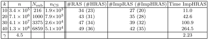
k n Nsub nCS #RAS (#HRAS) #ImpRAS (#ImpHRAS) Time ImpHRAS
10 3.4×10⁵ 216 1.9×10³ 34 (23) 27 (20) 11.0
20 7.1×10⁶ 1000 7.9×10³ 43 (31) 35 (28) 42.6
30 4.1×10⁷ 3375 2.6×10⁴ 47 (34) 39 (32) 100.9
40 1.3×10⁸ 6859 5.1×10⁴ 49 (36) 42 (35) 264.5
[image:7.612.133.470.173.237.2]γ 4.5 2.23
Table 2 δ∼2h,H∼Hsub∼k−0.8,κprob=κprec=k2.
α= 0.6 α= 0.8
k n Nsub nCS #2-level n Nsub nCS #2-level
10 2.6×10⁵ 27 2.8×10² 31 3.4×10⁵ 216 1.8×10³ 29
20 6.3×10⁶ 216 1.9×10³ 87 7.1×10⁶ 1000 7.9×10³ 60
30 3.3×10⁷ 343 2.9×10³ 148 4.1×10⁷ 3375 2.5×10⁴ 90
40 1.1×10⁸ 729 5.9×10³ 200 1.3×10⁸ 6859 5.1×10⁴ 154
β= 1 β= 2
k n Nsub nCS #2-level(Time) #2-level(Time)
10 3.4×10⁵ 216 1.8×10³ 29 (12.9) 37 (13.1)
20 7.1×10⁶ 1000 7.9×10³ 60 (63.7) 70 (69.8)
30 4.1×10⁷ 3375 2.5×10⁴ 90 (200.4) 101 (221.2)
40 1.3×10⁸ 6859 5.1×10⁴ 154 (771.7) 137 (707.6)
γ 4.5 2.4 1.2 (2.9) 0.94 (2.8)
ξ 1.0 0.5 0.3 (0.6) 0.2 (0.6)
Table 3 κprob =k,δ∼2h,H ∼Hsub ∼k−α,κprec =kβ; Top:β = 2, α= 0.6,0.8;
Bottom:α= 0.8,β= 1,2.
transmission conditions at the interfaces between subdomains are used in the preconditioner. It is important to note that the time is growing very much slower than the dimension of the problem being solved.
Experiment 3 In this case we take κprob = k. Moreover, we take
impedance boundary conditions on ∂Ω. We take H ∼Hsub∼k−α, κprec =
kβ, and we use ImpHRAS as a preconditioner.
In Table 3 on the bottom we see that the dimension of the coarse space is
nCS= (k−0.8)−3=k2.4=O(n0.5).
This is reflected in the γ and ξfigures in the nCS column. For this method
[image:7.612.163.445.265.429.2]The computation time grows only slightly faster than the dimension of the coarse space, showing (a) weak scaling and (b) MUMPS is still performing close to optimally for Maxwell systems of size 5×10⁴. Iteration numbers are growing with about n0.3 at worst. Note that the iteration numbers may be
improved by separating the coarse grid size from the subdomain size, making the coarse grid finer and the subdomains bigger.
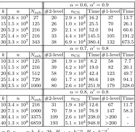
Experiment 4. Here we solve the pure Maxwell problem without ab-sorption, i.e. κprob = 0, with impedance boundary conditions on ∂Ω. In
the preconditioner we take κprec = k. Results are given in Table 4, where
Hsub∼k−α, H ∼k−α ′
. These methods are close to being load balanced in the sense that the coarse grid and subdomain problem size are very similar whenα+α′= 3/2.
Out of the methods tested, the 2-level method (ImpHRAS) with (α, α′ ) = (0.6,0.9) gives the best iteration count, but is more expensive. The method (α, α′
) = (0.7,0.8) is faster but its iteration count grows more quickly, so its advantage will diminish as k increases further. For (α, α′
) = (0.6,0.9) the coarse grid size grows withO(n0.64) while the time grows withO(n0.65). For (α, α′
) = (0.7,0.8) the rates areO(n0.54) and O(n0.69). The subdomain problems are solved on individual processors so the number of processors used grows askincreases. In the current implementation a sequential direct solver on one processor is used to factorize the coarse problem matrix, which is clearly a limiting factor for the scalability of the algorithm. The timings could be significantly improved by using a distributed direct solver, or by adding a further level of domain decomposition for the coarse problem solve.
AcknowledgementThis work has been supported in part by the French Na-tional Research Agency (ANR), project MEDIMAX, ANR-13-MONU-0012.
References
M. Bonazzoli, V. Dolean, I. G. Graham, E.A. Spence, and P-H. Tournier. Do-main Decomposition preconditioning for the high-frequency time-harmonic Maxwell equations with absorption. Submitted, arXiv:1711.03789, 2017. Y. A. Erlangga, C. Vuik, and C. W. Oosterlee. On a class of preconditioners
for solving the Helmholtz equation. Applied Numerical Mathematics, 50 (3):409–425, 2004.
M. J. Gander, I. G. Graham, and E. A. Spence. Applying GMRES to the Helmholtz equation with shifted Laplacian preconditioning: what is the largest shift for which wavenumber-independent convergence is guaran-teed? Numer. Math., 131(3):567–614, 2015.
α= 0.6,α′= 0.9
k n Nsub #2-level nCS Time #1-level Time
10 2.6×10⁵ 27 20 2.9×10³ 16.2 37 13.7
15 1.5×10⁶ 125 26 1.0×10⁴ 25.5 70 26.1
20 5.2×10⁶ 216 29 2.1×10⁴ 52.0 94 60.6
25 1.4×10⁷ 216 33 4.4×10⁴ 145.5 105 191.2
30 3.3×10⁷ 343 38 6.9×10⁴ 380.4 132 673.5
α= 0.7,α′= 0.8
k n Nsub #2-level nCS Time #1-level Time
10 3.1×10⁵ 125 28 1.9×10³ 8.2 58 7.7
15 1.5×10⁶ 216 39 4.2×10³ 19.0 82 20.1
20 6.3×10⁶ 512 58 7.9×10³ 42.4 123 49.7
25 1.4×10⁷ 729 60 1.7×10⁴ 80.6 148 94.1
30 3.5×10⁷ 1000 80 2.6×10⁴ 251.9 179 328.0
α= 0.8,α′= 0.8
k n Nsub #2-level nCS Time #1-level Time
10 3.4×10⁵ 216 31 1.9×10³ 12.6 67 11.7
20 7.1×10⁶ 1000 70 7.9×10³ 76.9 147 58.3
30 4.1×10⁷ 3375 109 2.6×10⁴ 238.0 >200
-40 1.3×10⁸ 6859 193 5.1×10⁴ 948.9 >200
-Table 4 κprob= 0,κprec=k,δ∼2h,Hsub∼k−α,H∼k−α′.
[image:9.612.191.411.93.309.2]