City, University of London Institutional Repository
Citation:
Bryson, A. and Forth, J. ORCID: 0000-0001-7963-2817 (2017). Wage Growth in
Pay Review Body Occupations. London, UK: Office of Manpower Economics.
This is the published version of the paper.
This version of the publication may differ from the final published
version.
Permanent repository link:
http://openaccess.city.ac.uk/20743/
Link to published version:
Copyright and reuse: City Research Online aims to make research
outputs of City, University of London available to a wider audience.
Copyright and Moral Rights remain with the author(s) and/or copyright
holders. URLs from City Research Online may be freely distributed and
linked to.
WAGE GROWTH IN PAY REVIEW BODY
OCCUPATIONS
Alex Bryson (UCL) and John Forth (NIESR)
Report to the Office of Manpower Economics
ii
DISCLAIMER
The views in this report are the authors’ and do not necessarily reflect those of OME.
THE AUTHORS
iii
TABLE OF CONTENTS
LIST OF FIGURES AND TABLES ... 5
ACKNOWLEDGEMENTS ... 6
ABBREVIATIONS ... 7
1. EXECUTIVE SUMMARY ... 8
1.1. Aims ... 8
1.2. Key Findings ... 8
1.3. Methodology ... 9
1.4. Findings in Detail ... 9
1.5. Implications ... 11
2. INTRODUCTION ... 13
2.1. Background to the research ... 13
2.2. The purpose and structure of this paper ... 14
3. AN OVERVIEW OF PROPENSITY SCORE MATCHING... 15
4. DATA CONSIDERATIONS WHEN IMPLEMENTING PSM TO COMPARE WAGE GROWTH IN PRB AND 'LIKE' OCCUPATIONS ... 17
4.1. Introduction to ASHE and QLFS ... 17
4.2. Defining a PRB occupation ... 17
4.3. Discontinuities in occupational coding over time ... 20
4.4. Constructing a Panel of Occupations ... 21
4.5. Earnings measures ... 22
4.6. Matching variables ... 24
5. METHODS FOR COMPARING WAGE GROWTH IN PRB AND NON-PRB OCCUPATIONS ... 26
5.1. Earnings Growth for PRB Occupations Relative to "Matched" non-PRB Occupations ... 26
5.2. What Accounts for Differential Earnings Growth in PRB and Matched non-PRB Occupations? ... 28
6. RESULTS ... 31
6.1. Descriptive Analyses of Earnings Change and Rank Earnings ... 31
6.2. PSM Estimates of Median Hourly Earnings Growth ... 35
6.3. Micro-analysis of Employees in Matched Occupations ... 45
7. SUMMARY AND CONCLUSIONS ... 48
8. BIBLIOGRAPHY ... 54
5
LIST OF FIGURES AND TABLES
Table ES1: Growth in Median Real Gross Hourly Earnings, 2005-2015 ... 10
Table ES2: Growth in Median Real Gross Hourly Earnings Having Netted Out Changes in Workforce Composition, 2005-2015 ... 11
Table 1: ASHE Employee Observations, By Year ... 18
Table 2: ASHE PRB Totals Relative to the OME Business Plan ... 20
Table 3: The Distribution of PRB Occupations By SOC Major Groups ... 22
Figure 1: Median Real Hourly Occupational Earnings, 2005-2015... 31
Figure 2: Growth in Median Real Occupational Earnings, 2005-2015 (2005=100) ………32
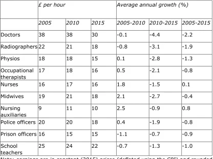
Table 4: Median Real Hourly Earnings (ASHE) for 10 PRB Occupations ... 33
Table 5: Occupational Rankings on Median Hourly Earnings ... 34
Figure 3: Change in Hourly Wage Rank and Annual Wage Growth ... 35
Table 6: Growth in Median Real Wages, PRB Nurses ... 36
Table 7: PSM Variable Means for PRB Nurses and their Comparators ... 37
Table 8: Growth in Median Real Wages, PRB Radiographers ... 38
Table 9: Annual Growth in Median Real Wages, PRB Physios ... 39
Table 10: Annual Growth in Median Real Wages, PRB Midwives ... 39
Table 11: Annual Growth in Median Real Wages, PRB Occupational Therapists .. 40
Table 12: Annual Growth in Median Real Wages, PRB Doctors ... 42
Table 13: Annual Growth in Median Real Wages, PRB Nursing Auxiliaries ... 42
Table 14: Annual Growth in Median Real Wages, PRB Teachers ... 43
Table 15: Annual Growth in Median Real Wages, PRB Police Officers ... 44
Table 16: Annual Growth in Median Real Wages, PRB Prison Officers ... 45
Table 17 Change in Hourly Median Real Wages 2005-2015 – Micro-Analysis ... 46
Appendix Table A1: PRB Occupations ... 57
6
ACKNOWLEDGEMENTS
We gratefully acknowledge funding from the OME who funded this work under their open call for research on public sector pay and workforces. We thank Jonathan Wadsworth, Ken Clark, Nicola Allison and participants at OME’s Research Conference for useful comments on an earlier draft.
This report presents research based on data from the Annual Survey of Hours and Earnings (ASHE) and the Quarterly Labour Force Survey (QLFS), both produced by the Office for National Statistics (ONS). The data are Crown Copyright and reproduced with the permission of the controller of HMSO and Queen’s Printer for Scotland.
We acknowledge the ONS as the owner and distributor of the ASHE and QLFS. Both were supplied by the Secure Data Service at the UK Data Archive.
The use of the ASHE and QLFS data does not imply the endorsement of the Secure Data Service in relation to the interpretation or analysis of the data. This work uses research datasets which may not exactly reproduce National Statistics aggregates.
7
ABBREVIATIONS
APS Annual Population Survey
ASHE Annual Survey of Hours and Earnings BSD Business Structure Database
CPI Consumer Prices Index
IDBR Inter Departmental Business Register NHSPRB National Health Service Pay Review Body OLS Ordinary Least Squares
OME Office of Manpower Economics ONS Office for National Statistics PRB Pay Review Body
PSM Propensity Score Matching QLFS Quarterly Labour Force Survey SIC Standard Industrial Classification SOC Standard Occupational Classification STRB School Teachers’ Review Body
8
1. EXECUTIVE SUMMARY
1.1. Aims
Individuals' incentives to enter or leave a profession – and their incentives to work productively – are partly driven by what they can earn in that occupation, compared to what they might earn in an alternative profession for which they are qualified. This study aims to arrive at a better understanding of how earnings growth for employees in occupations covered by the PRBs compares with the earnings growth of employees in other, similar occupations. The study:
describes earnings growth among Pay Review Body (PRB) occupations;
compares that growth to earnings growth in comparable non-PRB occupations;
accounts for differences in earnings trajectories between PRB occupations and comparable non-PRB occupations that come from compositional change in the workforces.
1.2. Key Findings
Averaging across all 353 occupations in the UK’s Standard Occupational Classification, there was a decline of 5.8% in median real gross hourly occupational earnings between 2005 and 2015.1 The decline was steeper among
non-PRB occupations than PRB occupations (6.1% compared to 3.1%).
Among the 10 largest PRB remit occupations, median real gross hourly occupational earnings fell 10.1%, on average, between 2005 and 2015. However, wage growth varied considerably across PRB occupations, even among occupations whose pay was set by the same PRB.
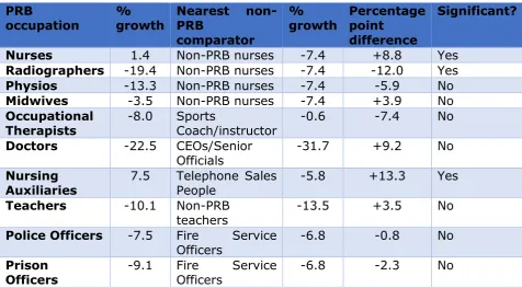
Relative to their nearest non-PRB comparators, earnings growth was higher for the PRB group in five cases and lower in five cases. However, differences were only statistically significant in three instances, with PRB Nurses and PRB Nursing Auxiliaries experiencing higher earnings growth than their non-PRB comparators, while PRB Radiographers experienced significantly lower growth than their non-PRB comparator occupation (Table ES1). Wage growth in a specific occupation may arise for a variety of reasons, including changes in the composition of the occupation (e.g. an influx of highly-qualified recruits). After accounting for compositional differences in the workers entering different occupations between 2005 and 2015, relative to their nearest non-PRB comparators, earnings growth was higher for the PRB group in seven cases and lower in three cases (Table ES2).
The degree to which earnings growth varies across occupations even within the PRB sector, and after accounting for workforce changes, is, perhaps, the biggest finding from the study. This is despite a fairly uniform public sector pay policy being applied to these groups over the latter half of the period.
1 Median rather than mean earnings growth was chosen to minimise the impact of
9
1.3. Methodology
Using data from the Annual Survey of Hours and Earnings (ASHE), together with the Quarterly Labour Force Survey (QLFS) we construct a panel of nearly 400 occupations. These data are used to examine growth in median real gross hourly occupational earnings in the PRB and non-PRB sectors over the period 2005-2015 before comparing wage growth in the ten largest PRB occupations with wage growth in “matched” non-PRB occupations. PRB occupations are “matched” to non-PRB occupations based on their characteristics in 2005. We identify the role played by workforce compositional change in the divergence in earnings paths between PRB and non-PRB comparable occupations.
1.4. Findings in Detail
Table ES1 presents growth in median real gross hourly earnings for the 10 largest PRB occupations and their non-PRB comparator occupations between 2005 and 2015. Table ES2 presents earnings growth in the same way, having netted out the effects of workforce compositional change in the PRB and non-PRB
comparator occupations.
The chief findings are as follows:
• PRB Nursing Auxiliaries experienced the highest absolute earnings growth, and the highest earnings growth relative to their non-PRB comparator. Their earnings gains were apparent having accounted for changes in occupational workforce composition.
• PRB Nurses experienced very low earnings growth, but it was significantly higher than the earnings growth experienced by their non-PRB comparator. However, the gap closes when accounting for changes in occupational workforce composition. Relative to their non-PRB comparator PRB Nurses experienced relative growth in the proportion working in London and the South East, increasing tenure and they were ageing more rapidly, all of which are conducive to relative improvements in earnings. • PRB Midwives experienced a small decline in earnings, one that was a little
smaller than that of their non-PRB comparator, although not significantly so. Accounting for changes in occupational workforce composition, they experienced earnings growth which was very similar to that of their non-PRB comparator.
• PRB Doctors have seen the biggest fall in median real gross hourly earnings out of the 10 PRB occupations, but the fall was not as large as that experienced by their non-PRB comparator. Furthermore, the decline is largely accounted for by compositional change among PRB Doctors, including a decline in their relative age and tenure. Having accounted for this the earnings growth PRB Doctors experience relative to their non-PRB comparator increases quite considerably.
10
doubled relative to its non-PRB comparator occupation having accounted for changes in occupational workforce composition.
• PRB Occupational Therapists’ earnings performed poorly relative to their non-PRB comparator occupation but this was wholly accounted for by changes in occupational workforce composition.
• PRB Teachers experienced real earnings decline which was slightly smaller than that experienced by its comparator occupation, non-PRB Teachers, but the difference is not statistically significant. For both occupations earnings decline is largely accounted for by changes in workforce composition.
[image:10.595.85.562.335.598.2]• Police Officers and Prison Officers experienced moderate earnings decline that was similar to that for their non-PRB comparator occupation. Accounting for compositional changes in their workforces reduced the rate of earnings decline a little for both PRB occupations, whereas it doubled the rate of decline for their non-PRB comparator occupation, improving the relative position of the two PRB occupations.
Table ES1: Growth in Median Real Gross Hourly Earnings, 2005-2015
PRB
occupation
%
growth
Nearest non-
PRB
comparator
%
growth
Percentage
point
difference
Significant?
Nurses
1.4
Non-PRB nurses
-7.4
+8.8
Yes
Radiographers
-19.4
Non-PRB nurses
-7.4
-12.0
Yes
Physios
-13.3
Non-PRB nurses
-7.4
-5.9
No
Midwives
-3.5
Non-PRB nurses
-7.4
+3.9
No
Occupational
Therapists
-8.0
Sports
Coach/instructor
-0.6
-7.4
No
Doctors
-22.5
CEOs/Senior
Officials
-31.7
+9.2
No
Nursing
Auxiliaries
7.5
Telephone Sales
People
-5.8
+13.3
Yes
Teachers
-10.1
Non-PRB
teachers
-13.5
+3.5
No
Police Officers
-7.5
Fire
Service
Officers
-6.8
-0.8
No
Prison
11
Table ES2: Growth in Median Real Gross Hourly Earnings Having Netted Out Changes in Workforce Composition, 2005-2015
PRB
occupation
%
growth
Nearest non-PRB
comparator
% growth Percentage
point difference
Nurses
8.6
Non-PRB nurses
6.4
+2.2
Radiographers
-13.9
Non-PRB nurses
6.4
-20.3
Physios
-7.4
Non-PRB nurses
6.4
-13.8
Midwives
6.1
Non-PRB nurses
6.4
-0.3
Occupational
Therapists
1.1
Sports
Coach/instructor
-0.9
+2.0
Doctors
-3.5
CEOs/Senior
Officials
-28.3
+24.8
Nursing
Auxiliaries
13.4
Telephone
People
Sales
-1.7
+15.1
Teachers
0.8
Non-PRB teachers
-2.9
+3.7
Police Officers
-6.3
Fire Service Officers
-13.4
+7.1
Prison
Officers
-4.9
Fire Service Officers
-13.4
+8.5
1.5. Implications
Earnings growth varies markedly across PRB occupations, even those whose pay is set by the same PRB. So it is important to understand earnings growth at the level of individual occupations. Comparing those movements to “like” non-PRB occupations is one way to assess whether PRB earnings growth is similar or different to what might have been anticipated given the position of PRB occupations in the earnings distribution and the nature of the workers undertaking the occupation. It is also possible to quantify earnings growth in PRB occupations relative to “like” non-PRB occupations having netted out the effects of compositional change in the individuals in those occupations.
There are various ways of identifying non-PRB comparator occupations. Previous studies use regression techniques to compare earnings in PRB occupations with other occupations, such as those in the rest of the public sector, or else they rely on “benchmarking” techniques based on case studies or qualitative assessments of occupational similarity. In this paper we have used propensity score matching to identify “nearest neighbours”. It has a number of strengths and weaknesses compared to methodologies used to date.
Its chief strengths are:
It permits comparison between specific occupations with similar characteristics, as opposed to broader comparisons made across groups of occupations.
It quantifies the “closeness” of comparators in a transparent fashion which other analysts can replicate and, potentially, improve upon.
In contrast to standard regression techniques it assists the analyst in avoiding comparisons with occupations that may not constitute good comparators to PRB occupations.
[image:11.595.87.565.119.345.2]12
It can be replicated over time to inform policy with up-to-date information.
By “balancing” PRB and comparator non-PRB occupational traits at the outset, one can argue that differences in subsequent earnings trajectories are independent of those observed traits at the outset.
Its chief weaknesses are:
It is reliant on data capturing occupational features that are liable to affect the outcome of interest, in this case earnings growth.
It can be sensitive to the methods used to estimate the metric for “closeness” and, having done so, the choices made as to which potential comparators to use.
Of course, the second of these weaknesses might also be perceived as a strength in the sense that it provides the basis for sensitivity analyses.
Regarding the first weakness, the data used in this paper do not contain information on job tasks: these may vary both within and across occupations and may drive some of the differences in earnings trajectories across PRB and comparator non-PRB occupations.
13
2. INTRODUCTION
2.1. Background to the research
Government and its agencies are reliant on recruiting and retaining high calibre staff to provide good quality public services, such as those offered by Pay Review Body (PRB) remit groups. In a market setting it is common for firms to pay efficiency wages or offer performance-related pay to attract the most-able employees in the labour market. The public purse places limitations on the public sector's ability to do this. Traditionally it has compensated by offering a good remuneration package including excellent occupational pensions, but this too is increasingly difficult given strictures on public finances and deferred payments such as pensions may not have a sizeable impact on employee recruitment. It is therefore timely to assess how earnings growth in PRB occupations compares with that in other "like" occupations and what the implications might be for rewarding PRB remit groups in future.
Individuals' incentives to enter or leave a profession – and their incentives to work productively – are partly driven by what they can earn in that occupation, compared to what they might earn in an alternative profession for which they are qualified. The motivation for the proposed research is then to arrive at a better understanding of how earnings growth for employees in occupations covered by the PRBs compares with the earnings growth of employees in other, similar occupations.
Recent PRB annual reports include assessments of how pay in their remit occupations compares with trends in other occupations. In most cases, there is some reference to national patterns of earnings growth (e.g. the ONS’ measure of Average Weekly Earnings). In some instances, reference is made to broad public/private sector pay differentials: for instance, the NHSPRB (2016) makes reference to the estimates produced by Jenkins (2014). Other PRB reports go further by making comparisons with particular groups of occupations: the STRB (2016) draws a comparison between the pay of schoolteachers and that of all other employees in SOC Major Group 2 (Professionals). Others make reference to one-off case studies (e.g. PA Consulting, 2008; Incomes Data Services, 2015) or the outcomes of job evaluation exercises (PWC, 2015).
14
proper account of differences in workforce characteristics and attributes, and differences in the labour market context surrounding employees in those occupations. The approach adopted in this study takes the issue of common support seriously, and also recognises that other things affect pay beyond the task content of occupations.
2.2. The purpose and structure of this paper
The paper outlines the methodology used to compare wage growth in PRB occupations with wage growth in "like" occupations between 2005 and 2015 and then, using that methodology, presents estimates of differences in wage growth between PRB occupations and their matched comparator occupations. Specifically, we:
Compile a panel of occupations covering the period 2005-2015 containing occupation-level average wages and average employee characteristics
Identify those occupations that are covered by PRBs and sets of matched comparator occupations that are not covered by PRBs
Chart the growth in median earnings in each of these occupations over the period 2005-2015, in order to examine how the earnings of the PRB groups have fared relative to the earnings in occupations that are observationally similar
Identify how much of the differential movement in average earnings between the PRB groups and their matched comparators is due to changes in their observed characteristics.
15
3. AN OVERVIEW OF PROPENSITY SCORE MATCHING
In this section we briefly review the existing literature on earnings and earnings progression for PRB occupations before turning to the value of propensity score matching (PSM) as a means of comparing earnings in PRB occupations with those for matched comparator occupations.
To date the literature used to shed light on earnings and earnings growth in PRB occupations has tended to estimate pay differentials between public and private sector employees as a whole (e.g. Jenkins, 2014; Cribb et al., 2014) or else compared PRB occupations with others in the public sector (Dolton et al., 2015). Regression-adjustments are made to account for the fact that differences in the demographic profile of employees in those occupations may also influence earnings growth. The difficulty with this standard approach is the occupational heterogeneity within both the private and public sectors, which means that earnings growth in specific PRB occupations, or groups of PRB occupations, is being compared with that in occupations which may have very different attributes. For instance, PRB employees remit groups are largely confined to SOC Major Groups 1, 2, 3 and 6, whereas the regression approaches cited above typically also include employees from SOC Major Unit Groups 4, 5, 7, 8 and 9.
"Matching" PRB occupations with non-PRB occupations according to their observed traits offers greater prospects of comparing wage trajectories for PRB occupations with "like" non-PRB occupations. "Likeness" is determined by characteristics of the occupations measured in 2005 which is the start of the period under investigation (2005-2015). It involves identifying occupations that are observationally similar to the PRB occupation, in terms of the sorts of individuals who work in them, where they sit in the earnings rankings, and their earnings trajectory in the years prior to 2005. Having done so one can argue that differences in earnings trajectories between the PRB and “like” non-PRB occupation subsequent to 2005 are independent of their observed characteristics at the outset.
We match non-PRB occupations to PRB occupations using a single index, the propensity score, which captures the degree of likeness between occupations based on their observed traits. The procedure allows us to establish how close particular occupations are to PRB occupations and to use this information to identify similar occupations, or sets of occupations, against which to judge the earnings growth of the PRB occupations. Those occupations deemed too far distant from the PRB occupation on the propensity score are excluded from the analysis since they are deemed insufficiently similar to the PRB occupation to constitute a credible comparator. The method avoids comparisons between earnings trajectories for PRB occupations and dissimilar non-PRB occupations, as occurs when all occupations or all workers are entered into a regression analysis.
16
Rosenbaum and Rubin (1983) showed that matching on a single index reflecting the probability of participation could achieve consistent estimates of the treatment effect in the same way as matching on all covariates. This index is the propensity score and this variant of matching is termed “propensity score matching”. The advantage is that it replaces high-dimensional matches with single index matches.
It is possible that occupational matches may not be found for one or more PRB occupations where the estimated propensity scores for non-PRB occupations are deemed insufficiently similar to those of the PRB occupations. In the literature these PRB occupations would be described as being "off common support", common support being that part of the propensity distribution for which comparator occupations are available. In this scenario it is not possible to recover a comparator for the PRB occupation. The analyst is able to set tolerances regarding the "nearness" of matching occupations, testing the sensitivity of results to the chosen bandwidth.
The explicit acknowledgement of the common support problem is one of the main features distinguishing PSM from regression analyses since regression results can be used to extrapolate to unsupported cases, something which may or may not be deemed appropriate. The other main distinguishing feature is that matching is non-parametric. Consequently, it avoids the restrictions involved in models that require the relationship between characteristics and outcomes to be specified. If one is willing to impose a linear functional form, the matching estimator and the regression-based approach share the same identifying assumptions.
17
4. DATA CONSIDERATIONS WHEN IMPLEMENTING PSM TO COMPARE WAGE GROWTH IN PRB AND 'LIKE' OCCUPATIONS
In this section, we describe the data sets used in the analysis, and how we approach the data issues that arise in identifying PRB occupations and their comparators.
4.1. Introduction to ASHE and QLFS
The Annual Survey of Hours and Earnings (ASHE) is a panel data set constructed from a survey of 1% of all employees in employment. Their employers are surveyed each April and asked to provide a wide range of information about the employee. Employees can be followed from year to year within the data, and job mobility can be identified through changes in the unique employer identifier. The survey is carried out by the UK’s Office for National Statistics (ONS) and is mandatory.
At the time the analysis was conducted, the ASHE data were available via the Secure Data Service for the period 1997-2015, however we confine our attention to the decade from 2005-15. This allows us to focus our analyses and findings on a relatively recent period – encompassing some years prior to the recession, when public sector employment was expanding, as well as more recent years when it has been contracting. There is also a practical aspect to our chosen observation period, as our prior work with ASHE indicates that changes to the design and wording of the questions on performance-related payments in 2005 mean that the incidence and extent of performance-related pay was understated in the years leading up to this change, thereby compromising any measure of total earnings.
Although it is common to use QLFS data to examine earnings and public/private sector differentials, ASHE has a number of benefits including a large sample size compared to QLFS, a long individual-level panel component, very high response rates, and accurate employer-provided data on both earnings and public versus private sector status.2 The main disadvantages of ASHE compared with QLFS are
its limited information on demographic characteristics and its hours measure, which is confined to paid hours.
4.2. Defining a PRB occupation
OME estimates suggest that the PRB system covers around 2.5 million workers, accounting for around 45% of all public sector employees (Office of Manpower Economics, 2015). All of these PRB workers have the potential to appear in ASHE, with the exception of: (i) the self-employed3 (ASHE covers employees only); (ii)
2 One important drawback with QLFS is that many respondents lack information
on these key data items when answering the survey, leading to measurement error. This problem is particularly acute with proxy respondents. For an example using information on trade union membership see
http://www.wiserd.ac.uk/research/civil-society/economic-austerity-social- enterprise-equality/trade-union-membership-associational-life-and-wellbeing1/research-findings/research-briefs/
3 Some General Medical Practitioners and General Dental Practitioners covered by
18
the Armed Forces; (iii) any employees working in Northern Ireland (the ASHE dataset available in the Secure Data Service only includes workplaces in Great Britain).
We focus our attention on occupations within the PRBs with the largest ASHE coverage, namely: NHS staff; School teachers; Doctors and Dentists; Police Officers; and Prison Service Staff. The Data Appendix lists all of the occupations within the remit of these five PRBs and specifies the means by which we identify PRB jobs within ASHE. We identify 33 separate occupational groups under these PRBs (see Appendix Table A1). They are variously identified using their four-digit occupational coding, their public sector status4, their location and, in some cases,
their SIC code.
[image:18.595.90.283.415.656.2]For occupations, such as teachers, where there are practitioners both within the PRB system (those in state schools) and those outside it (private schools), we use the SOC2010 unit group in combination with the IDBR legal status to identify those working in the public sector. Where an occupation code covers a group of jobs across different industrial activities (e.g. SOC2010=1173, which covers fire, ambulance and prisons) we use SIC(2007) in addition to identify the remit group (in this case, senior operational managers in the prison service). We also have regard to region, as some PRBs only cover England and Wales while others extend to Scotland.
Table 1: ASHE Employee Observations, By Year
YEAR OBSERVATIONS
2002 161,000
2003 163,000
2004 163,000
2005 165,000
2006 166,000
2007 139,000
2008 140,000
2009 171,000
2010 173,000
2011 183,000
2012 177,000
2013 180,000
2014 183,000
2015 180,000
In some cases, we cannot say with certainty whether an employee in ASHE is within the PRB's remit. Schoolteachers are one example, as it is not possible in ASHE to identify teachers in state-maintained schools (who are covered by the
4 The public sector identifier in ASHE is taken from the Inter-Departmental
19
STRB) from those in Academy schools (who, strictly speaking, are not).5 In the
case of medical practitioners and dentists, we have included those working in the private sector so as to capture those supplying services to the NHS under independent contracts.6
For the most part occupations within PRBs' remit have been so throughout the period of observation. However, there are occupations that have moved into or out of their remit, most notably the police whose pay has been set following PRB recommendations since 2014. We have chosen to set occupations as "PRB" or "not PRB" according to their status at the end of our period, namely 2015, such that changes in PRB status prior to that point are ignored. The reason for this is that the purpose of the study is to compare earnings growth in occupations that are currently within the PRBs' remit relative to comparator occupations. Our aim is not to establish whether PRBs have a causal effect on wage growth (an exercise which would rely on tracking occupational "switchers" over time).
Over the period of our analyses (2002 to 2015) ASHE provides around 2.3 million employee job observations, including 1.9 million for the main period of analysis between 2005 and 2015,7 with the sample size ranging between 139,000 and
183,000 employee job observations per year (Table 1). Of these, we identify around 18,000 jobs per year as PRB jobs using the definitions set out in the Data Appendix.
Our sample of PRB jobs in ASHE is slightly larger than anticipated when grossed up to population totals. If one grosses up our sample of jobs in 2015 using the ASHE population weights (CALWGHT), one arrives at an estimated total of 2.7 million jobs, accounting for 44% of the 6.1 million public sector jobs covered by ASHE (compared with the OME’s estimate of 2.5 million jobs cited earlier).8 Table
2 compares our 2015 ASHE estimates for PRB jobs with the headcounts cited in Figure 1 of the OME’s 2015-16 Business Plan (Office of Manpower Economics, 2016). The largest discrepancies arise in respect of the Police (where we estimate a total of 211,000 jobs rather than 137,000)9 and the NHS (with a
5 Under the ONS public sector definition academy schools are identified as being
in the public sector so they are indistinguishable from teachers in local authority controlled schools, despite the fact that academy school teachers are not within the PRB's remit.
6 In practice, this may include some private practitioners who perform no NHS
work and who are therefore not covered by the PRB. We do not have the information to estimate the size of this private practitioner group.
7 The 2002 to 2005 period was used for estimating earnings trajectories prior to
the main analysis period.
8 The share of public sector jobs that are PRB jobs has risen sharply in recent
years, from a stable 35% over the period 2005-2011. This is chiefly due to a decline in the numbers of non-PRB jobs in the public sector over the period since 2011. The rise is not an artefact of the switch to SOC(2010) coding because the increase does not occur until after 2011.
9 It is difficult to explain the discrepancy. There are single SOC codes for senior
20
[image:20.595.94.384.171.263.2]300,000 discrepancy). A comparison with the APS reveals that its occupational totals are closer to those published by OME for these two PRBs, but that its estimates are further away for the remaining three PRBs. It is then clear that there is no firm consensus on the size of the various remit groups.
Table 2: ASHE PRB Totals Relative to the OME Business Plan
PRB totals
ASHE 2015
OME Business Plan 2015-16
Doctors and dentists
197,000
212,000
NHS
1,708,000
1,408,000
Police
211,000
137,000
Prisons
29,000
27,000
School teachers
512,000
540,000
Some measurement error in designating certain employees as within the PRBs' remit is unavoidable, as in the case of Academy school teachers noted above. One issue that bedevils research relying on the designation of employees as either public or private sector workers is measurement error in the recording of public sector status. This occurs because workers are often not well informed about the public sector status of their employer. However, ASHE relies on quality-assured administrative data from the IDBR to identify the status of the workplace, thus minimising this measurement error problem (Millard and Machin, 2007; Dolton et al., 2015). Similarly, as shown in the Data Appendix, some PRBs cover England and Wales, while others also cover Scotland, yet employer location is coded without error in ASHE by the employer who provides the full postcode for the workplace where the sampled employee works. Some PRBs also cover Northern Ireland, but the ASHE data in the Secure Data Service does not.
There are therefore disagreements between different sources as to the total number of jobs that fall under the remit of these five PRBs. However, the causes of the discrepancies between the different sources are difficult to identify without further information on the totals published by OME.
4.3. Discontinuities in occupational coding over time
Occupations are relatively static over time, in the sense that the bundle of tasks performed within an occupation, coupled with the socio-economic status that is also accounted for in the coding of occupational hierarchies, is quite stable. That said, the range of job tasks in the economy – and how these are bundled into jobs - do change over time, leading to new occupational classifications. (Some occupations are born, some die, while others grow or shrink in importance).
21
For non-PRB unit groups, we collapse the ASHE data to SOC(2010) unit group level in those years when SOC(2010) is available and we use the ONS’ occupational look-up tables (Office for National Statistics, 2012) to construct SOC(2010) Unit Groups from the SOC(2000) data in the years prior to 2011. This allows us to create a dataset of continuous occupational classes.
The Office for National Statistics (ONS) occupational look-up tables utilise data from three surveys which have been coded to both SOC(2000) and SOC(2010), specifically: the 1996/7 QLFS; the January to March quarter of the 2007 QLFS; and a 1% sample of economically active respondents from the 2001 Census. In each of these dual-coded datasets, ONS have cross-tabulated the SOC(2000) code and the SOC(2010) codes for each individual to arrive at a set of tables which show how the two classifications map onto one another. Separate tables are created from each dataset at Major Group (one-digit), Sub-Major Group (two-digit), Minor Group (three-digit) and Unit Group (four-digit) level, and each tabulation is done separately for men and women. We have used the Unit Group level tables deriving from the 2001 Census sample, as the sample size for the dual-coded data is three times the size of that used in the QLFS dual coding (circa 210,000 observations, compared with ~67,000 for the 2007 QLFS).10
We use the male and female Census correspondence tables at Unit Group (UG) level to derive a set of weights for each SOC(2000) UG which show that UG’s contribution towards the composition of each specific SOC(2010) unit group. For instance, Table 1a in ONS (2012) shows that, in the 2001 Census sample, some 26.7% of the men in SOC(2000) UG 1111 and 20.8% of the men in SOC(2000) UG 1113 were coded to SOC(2010) UG 1116 (these being the only SOC(2000) UGs with men classified to that SOC(2010) UG). The equivalent figures for women were 11.1% and 21.7% respectively. We are then able to construct SOC(2010) UG 1116 in our ASHE data prior to 2011 by taking 26.7% of the men coded to SOC(2000) UG 1111, 20.8% of the men coded to SOC(2000) UG 1113, 11.1% of the women coded to SOC(2000) UG 1111 and 21.7% of the women coded to SOC(2000) UG 1113, and combining these individuals together as one group.11
4.4. Constructing a Panel of Occupations
The procedure outlined above allows us to create a panel of SOC(2010) UGs from ASHE over the period 2005-2015, even though many of those years of ASHE data are coded to SOC(2000). Anyone in a PRB SOC group who is not actually covered by a PRB, such as secondary school teachers in private schools, constitutes an additional occupational group in our data represented by a new row in our occupational panel. That is to say, when a UG contains PRB covered and non-covered employees we create separate rows of data for each (one PRB row and one non-PRB row for teachers, in this case).12 In principle, among the PRB
10 The correlation between the unit group weights is nonetheless high across
these two sources (0.96 for men and 0.95 for women).
11 In practice, we do not ‘take’ 26.7% of the individuals, but give them a weight
equal to 0.267 times their ASHE population weight when computing aggregated estimates for the SOC(2010) UG, using a Horwitz-Thompson type estimator.
12 We had originally intended to separately identify Head Teachers but they are
22
occupations all but police officers may have non-PRB employees in the same occupation. The remaining rows of the panel consist of occupational unit groups where nobody has their pay set via a PRB.
In collapsing the ASHE data to occupation level the data are weighted with ASHE population weights (the variable is called CALWGHT).
[image:22.595.95.423.263.443.2]Our final balanced panel contains 394 SOC(2010) Unit Group occupations. Of these 32 are PRB occupations (see Appendix Table A1) and 362 are non-PRB occupations. They are observed over 11 years providing us with 5,516 occupation-by-year observations.
Table 3: The Distribution of PRB Occupations By SOC Major Groups
SOC Major
Group
Number of
non-PRB occupations
Number of PRB
occupations
Total
% PRB
1
35
3
38
8%
2
68
15
83
18%
3
62
5
67
7%
4
25
1
26
4%
5
57
1
58
2%
6
26
4
30
13%
7
18
1
19
5%
8
42
1
43
2%
9
29
1
30
3%
All
362
32
394
8%
A cursory glance at the occupational distribution of PRB occupations reveals that they are more heavily concentrated in SOC Major Group 2, 3, 1 and 6 than their non-PRB counterparts (Table 3). In 2015 64% of PRB employees were in SOC(2010) Major Group 2 compared with just 15% of non-PRB employees, bringing us back to our earlier point about the importance of identifying observationally similar comparators.
4.5. Earnings measures
Our analysis of wage growth focuses on changes in median gross hourly earnings among employees in each of our chosen occupations.
Employers of the sampled ASHE employees are asked to provide a wide range of information about the employee's earnings during the preceding year, including the amount of bonus or incentive pay received. The survey also asks about the employee's earnings and hours during the current pay period (that is, the week that includes the survey date, for employees paid weekly, or the month including the survey date for those paid monthly). From these data we are able to derive alternative measures of employees' gross hourly earnings.
23
We focus on the measures of earnings that relate to the preceding year ie. gross annual earnings, rather than merely the current pay period, in order not to miss any bonus payments that are not paid in the pay period covered by ASHE’s April survey date. Forth et al. (2016) show that bonuses are highly seasonal. A focus on the April pay period alone thus risks understating the importance of bonus payments, and is likely to do so differentially across occupations and industries.
Our analyses focus on hourly pay rather than annual or weekly earnings for both full-time and part-time employees, so that our comparisons are unaffected by differences between occupations in the average numbers of hours worked per week or per annum. Our measure of hourly pay is constructed from total gross annual earnings13 but relies on a measure of hours worked from the reference
period to convert this to an hourly rate, as ASHE contains no data on annual hours. Our assumption, then, is that hours in the reference period (April) are a good proxy for average annual hours.14
Earnings data perform two functions. First, we match PRB occupations with their non-PRB comparators using 2005 gross hourly earnings and changes in gross hourly earnings between 2002 and 2005. Second, earnings growth from 2005-2015 is our dependent variable.15 Measures used to capture pre-2005 pay trends
include some measurement error because they rely on the “old” set of ASHE questions on performance-related pay, as noted earlier.16
In tracking earnings growth since 2005 we adjust nominal earnings for price inflation using the Consumer Prices Index (CPI, with 2015=100) so that earnings growth is measured in terms of real wage growth since 2005.
13 Throughout we use the terms wages and earnings interchangeably but, strictly
speaking, we are estimating earnings not wage rates.
14 We tested this assumption using the Annual Population Survey (APS) to see
how hours varied across the year. In fact, March/April hours are typical. The average number of hours worked in March and April 2015 combined was 35.46 a week, compared with an annual average of 35.48 a week. Thus, it appears that using hours in April to characterise hours worked over the course of a year is relatively unproblematic.
15 To establish whether median occupation-level earnings may have been affected
by the construction of occupational groups crossing the change in SOC classification in 2010/11 we investigate the correlation between median occupation-level wages within the “real” and “synthetic” SOC(2010) groups in 2011 when data were dual coded. The correlation is 0.94 for all occupations and 0.97 for PRB occupations and there is no systematic bias upwards or downwards.
16 The question about annual incentive pay was first introduced into ASHE in
24
Throughout we analyse growth in median hourly earnings, as opposed to mean earnings, so our estimates are not so sensitive to changes in within occupation earnings dispersion.
4.6. Matching variables
The ability of PSM to identify occupations that are closely matched to PRB occupations at the start of the period relies upon the assumption that, conditional on the observed traits used in the matching algorithm, subsequent earnings growth in the absence of a PRB is independent of whether an occupation has its pay set via a PRB. This conditional independence assumption is not testable but its credibility can be considered in the light of theoretical considerations relating to wages growth. Factors that are likely to affect PRB status and earnings outcomes include the human capital of the workers in that occupation, as indicated by their age, education, and gender, other demographics such as ethnicity, and the location of workers (which will likely reflect wage demands and local cost pressures). These are included in our matching estimator.
We also match on earnings growth in the period 2002-2005 and earnings levels in 2005 to ensure that the baseline earnings of PRB and matched non-PRB occupations are very closely matched. By accounting for variations in pre-2005 earnings trends we minimise the potential for post-2005 earnings growth to reflect the statistical artefact of regression to the mean, that is, a period of low earnings growth is likely to be followed by a catch up and vice versa. These pre-2005 earnings data can also help capture otherwise unobservable occupation-specific factors that might drive occupational earnings growth.
Finally, in order to restrict our comparisons to occupations at a similar point in the occupational hierarchy, we require comparator occupations to be drawn from the same SOC Major Group or a Major Group adjacent to it.
Age, gender, location, earnings in 2005 and earnings change between 2002 and 2005 are derived from ASHE. Although location can be very precisely identified we focus on the key distinction between London and the Rest of the South East and elsewhere.
Other variables on employee demographic traits and qualifications are derived for the relevant SOC unit group using the APS.17 For instance, as education is not
recorded in ASHE we match on estimates of the distribution of employees in each occupation by education (using the levels of the National Qualifications Framework or NQF) from the APS. The education coding distinguishes between NQF Levels 0-4 (“no degree”), NQF Levels 4-6 (“lower degree”) and NQF Levels 7-8 (“higher degree”); those with vocational qualifications are coded according to their NVQ level attainment.18 These data are used in our matching estimators, but
we also look at variations in educational attainment over time as one potential explanation for movements in earnings.
17 The APS suffers from similar problems to the LFS mentioned earlier, including
measurement error associated with public sector status.
18 We use the APS variable HIQUAL11 (and its predecessors), categorising codes
25
We experimented with various specifications for the model estimating the probability of being the PRB occupation but, in the end, chose a relatively simple model containing the following occupation-level variables:
Percent male
Mean number of children (including zeros)
Mean age
Percent married
Percent white
Percent with a highest qualification at Masters level or above and percent with a highest qualification at undergraduate degree level (with these coefficients evaluated against a reference group, namely the percent with a highest qualification below degree level)
Percent working in London or the South East
Percent working in a large organization (with 10,000 or more employees)
Median annual hourly earnings in 2005
Whether median real annual earnings grew between 2002 and 2005
Demographic characteristics often affect occupational choices, as well as earnings, so it makes sense to incorporate them in the model. Investments in human capital through the education system will also influence occupational choices and earnings. Some PRB occupations such as teaching require occupation-specific qualifications. Both size of organization and region are known to be associated with earnings. Although it is less clear what role they have in relation to being a PRB occupation, it seemed sensible to incorporate them in the matching estimator. Finally matching on median occupational earnings in 2005 and trends in median real occupational earnings between 2002 and 2005 ensures that comparators for the PRB occupations are likely to be drawn from the sub-set of occupations resembling the PRB occupation in terms of where the occupation sits in the earnings distribution at the start of our period of analysis (2005), as well as sharing similar earnings’ trajectories prior to the analysis period.
Descriptive information on these variables is given in the top half of Appendix Table A2 for all 392 occupations that appeared in the balanced panel. Minimum and maximum values are omitted to avoid disclosure.
26
5. METHODS FOR COMPARING WAGE GROWTH IN PRB AND NON-PRB OCCUPATIONS
In this section we describe the methods used to compare wage growth for the median earnings in a PRB occupation to that for median earnings in “like” occupations, using propensity score matching (PSM). We describe how we implement PSM to estimate differences in earnings growth between PRB occupations and their matched comparator occupations, explaining the choices we made in the process, and comment on the assumptions that underpin the approach adopted. We also describe how we use regression techniques to establish the degree to which workforce compositional change can account for differences in occupational earnings growth between PRB occupations and their matched comparators.
5.1. Earnings Growth for PRB Occupations Relative to "Matched" non-PRB Occupations
We compare growth in log hourly median earnings in PRB and comparable non-PRB occupations having matched the non-PRB to non-non-PRB occupations using propensity score matching (PSM) (Rosenbaum and Rubin, 1983; Bryson et al, 2002). We match PRB occupations to non-PRB occupations according to their characteristics in 2005 to ensure that we are comparing earnings growth over the period 2005-2015 for occupations that started from a similar point in the earnings distribution and had a similar demographic make-up. If PSM leads to a satisfactory match between a PRB occupation and a comparator non-PRB occupation or occupations this will be apparent from the balance between the values on the matching variables between the PRB and non-PRB occupations. If this is satisfactory according to metrics discussed below, and one believes that the covariates used in the matching capture the main features affecting both the propensity to be a PRB occupation and earnings growth, we can recover the wage growth in the PRB occupation relative to a “like” non-PRB occupation, or occupations, by simply comparing the difference in the log median earnings growth of the PRB occupation and its matched comparator(s).
Our first consideration was which occupations to include in the matching estimates. It is impractical to look at each of the 32 PRB occupations that we can track over time in detail. In any event, some of them contain relatively few observations making estimation imprecise. We therefore adopted the following criteria for the inclusion of PRB occupations in our PSM analysis:
The occupation needed to be a well-defined group, that is, a single unit group, which meant ignoring some of the NHS occupational groups that were ill-defined in terms of their SOC code. The exception was teachers who, although they spanned four SOC unit groups, are nevertheless a homogeneous set
The occupation must contain a minimum threshold of 150 employee observations per annum, on average, over the period 2005-2015 to ensure precise estimates (and to avoid problems relating to the inadvertent disclosure of sensitive data)
27
This resulted in the identification of the 10 occupations marked in yellow in Appendix Table A1. Together they accounted for 70% of PRB employees in 2005, rising to 75% in 2015.
It seems sensible to ensure that there are a reasonable number of employee observations in each potential non-PRB comparator occupation so we confine our attention to those 222 non-PRB occupations with at least 150 employees in 2005, which is the point in time at which the occupations are matched.
Having identified the sample of occupations for inclusion in the analysis the next stage is to run matching estimates for each of the 10 PRB occupations separately. This involved two steps. First, we chose to “hard match” on SOC Major Group, that is, we decided that matched comparators to the PRB occupations had to be drawn from the same part of the SOC Major Group distribution – either they had to come from the same SOC Major Group or the Major Group adjacent to it. For example, PRB nurses belong to SOC Major Group 2 so matches are only sought in SOC Major Groups 1, 2 and 3.19 Having done this, matching is run for the 10 PRB
occupations separately. This entailed running an OLS regression with covariates measured in 2005 (together with earnings growth over the period 2002-5) on a dummy variable identifying the PRB occupation.20 We then recover each
occupation’s probability of being the PRB occupation under the model. This predicted probability is the propensity score which is used to calculate the distance between each non-PRB occupation and the PRB occupation.
The resulting propensity score is fed into the matching estimator to recover a matched comparator or comparators giving greater weight to those Unit Groups that are close to the chosen PRB occupation in terms of observables, and less weight to those that are more distant. In the process, some Unit Groups may be omitted from the matched sample where the estimated propensity score is too distant. In this way, one arrives at a combination of Unit Groups which is observationally equivalent to the chosen PRB occupation at the start of our period of study, and which can then be used as matched comparators for that occupation.
We used the STATA algorithm PSMATCH2 for this process. There are a range of options available to the analyst in deciding which occupations should constitute matched comparators for the PRB occupation. These choices entail trade-offs between estimators that are the least biased and those that use the data more efficiently (Bryson et al., 2002: 26-28). Nearest neighbour matching bases comparisons of PRB earnings growth with that of the occupation that is closest to it in the propensity score distribution, thus delivering the least-biased estimates at the expense of throwing away information related to other occupations closest to the nearest neighbour. However, following Frölich et al. (2015), we also report results using the five nearest neighbour occupations to construct the non-PRB
19 In practice this means comparators cannot be drawn from a part of the
occupational distribution that is far from the PRB’s position in the occupational distribution.
20 Ordinarily estimates of the propensity score are based on a probit or logit
28
counterfactual.21 Nearest neighbour matching has the additional advantage of
identifying a specific occupation whereas using the five nearest neighbours entails comparing PRB earnings growth to a synthetic composite occupation. By using two sets of estimates – the nearest neighbour and the nearest five neighbours – we can establish how sensitive our results are to alternative choices. We compare these estimates to those derived from a simple naïve comparison between wage growth in the PRB occupation and the average among all non-PRB occupations taken together.
We investigate the quality of the occupational matches to ensure that covariates are reasonably balanced across PRB and non-PRB occupations post-matching. We do so using a standard technique which involves computing for each matching covariate the absolute deviation of the comparator occupation(s) from the PRB occupation, standardising this distance by expressing it as a proportion of the value for the PRB occupation. These deviations are then summed across all covariates to obtain an absolute standardised bias measure. We compare this measure of bias for the three cases, namely the naïve comparison between the PRB occupation and all non-PRB occupations, the nearest neighbour estimates and the five nearest neighbour estimates, to establish what effect matching has in reducing the absolute standardised bias.
To establish whether the difference between PRB earnings growth and that of its matched comparator(s) is statistically significant it is necessary to obtain standard errors for those estimates. We recover these standard errors for the nearest neighbour estimates by constructing an employee level data set containing only employees in the PRB occupation and its nearest neighbour for the years 2005 and 2015. We recover the difference in earnings growth for those employees by using quintile regression and interacting the PRB indicator with a year dummy for 2015. This returns the differential wage growth at the median for those in the PRB occupation relative to its nearest neighbour together with a standard error for that coefficient.
5.2. What Accounts for Differential Earnings Growth in PRB and Matched non-PRB Occupations?
Wage growth in a specific occupation may arise for a variety of reasons, including changes in the composition of the occupation. For instance, an increase in the qualification levels of the average employee or a shift in employment to higher-cost areas such as the South East are both likely to increase average wage levels within an occupation. Similarly, recruitment drives which bring in large numbers of inexperienced recruits are likely to lower the average wage level, as these individuals are likely to be on lower pay.
We seek to establish whether such compositional changes can account for any differential occupational earnings growth between PRB and “matched” occupations over the past decade. We do this by using regression methods to estimate the aggregate effects of compositional change on occupational earnings within our panel of 232 occupations. The coefficients from that regression are then used to estimate how compositional change affected earnings growth within each of our PRB occupations.
21 In their simulations Frölich et al. (2015) found that one-to-many matching was
29
The methodology for doing this is as follows. First, we run a regression model estimating log hourly median wage changes between 2005 and 2015 for all 232 occupations used in the PSM analysis (10 PRB occupations and 222 non-PRB occupations). The model contains variables capturing changes in the composition of workers in each of these occupations over the period 2005-2015. The variables used are those with the “d” prefix in the bottom half of Appendix Table A2. They are changes in:
proportion male;
mean age;
mean tenure;
educational qualifications (proportion with Master’s degree or above and proportion with an undergraduate degree)
contractual arrangements (proportion full-time; proportion on temporary contracts; proportion in performance pay jobs);
receipt of additional payments (overtime; shift premia; performance-related pay; employer pension contributions22);
union pay setting;
occupational entry and exit rates;
inter-firm mobility rate;
average firm size;
proportion located in London and the South East.
These variables are all known to influence earnings and earnings growth, either because they capture aspects of employees’ human capital (male, age, tenure, qualifications), firms’ ability to pay (firm size), local labour market conditions (geographical location), job amenities which employees may trade-off against wages (contract type, additional payments), or the operation of internal and occupational labour markets (inter-firm mobility rates and occupational entry and exit rates).
Changes in these variables account for around two-fifths of the change in log median occupational earnings between 2005 and 2015.23 Occupations experience
higher growth in earnings when they experience increases in the proportion male, the age of their workers, their tenure, their qualifications, the proportion on permanent contracts, the proportion in performance pay jobs, and the proportion working in London and the South East, and with a reduction in the proportion in receipt of overtime payments.
22 Pensions fall largely outside the remit of PRBs. However, as Dolton et al.
(2015) make clear, a total reward approach to comparability across occupations would need to take account of pension entitlements. These have traditionally been more generous in the public than the private sector. It is therefore conceivable that PRB occupations that appear to be less well-paid than their non-PRB occupational counterparts are, in fact, relatively much better off once one accounts for differences in pension entitlements. ASHE does not contain pension entitlement data but it does contain information on pension contributions made by employers which are strongly correlated with pension entitlements and used here to partial out changes in occupational pension contributions when comparing residual wages between PRB and non-PRB occupations.
30
From this regression we can recover wage growth having netted out the contribution from compositional changes along the dimensions listed above. We call this ‘residual wage growth’ since it is wage growth that is not accounted for by the variables listed above.24 We compare these residual wage changes
between PRB occupations and their matched comparator occupations using the approach described in Section 5.1. In so doing, we obtain an estimate of the extent to which differential earnings movements between the PRB occupation and its matched comparator can be explained by differential changes in the composition of those occupations (and thus an estimate of the extent to which differential earnings movements remain unexplained).
A comparison of earnings growth and growth in residual earnings between PRB occupations and their matched comparators allows us to estimate the degree to which compositional changes between 2005 and 2015 noted above account for the differences in wage trajectories in PRB and non-PRB occupations. The gap that is unaccounted for by compositional change could be said to approximate the “true” underlying differences in earnings trajectories between PRB and other occupations.
24 Residual wage growth is highly correlated with unadjusted wage growth: the
31
6. RESULTS
In this section, we present our findings on occupational earnings growth for PRB occupations relative to non-PRB occupations. We begin with descriptive analyses of earnings growth and relative earnings between 2005 and 2015 before turning to PSM estimates of earnings growth for 10 PRB occupations relative to matched comparator non-PRB occupations.
6.1. Descriptive Analyses of Earnings Change and Rank Earnings
Figure 1 shows the change in the arithmetic mean of median real gross hourly occupational earnings that occurred between 2005 and 2015 with earnings indexed to 100 in 2005. The graph is run for all 394 occupations appearing in the balanced panel and thus shows the average (mean) value of all 394 occupation-level medians in each year. It is striking that for all occupational groupings real earnings begin falling from 2010 and remain well below their 2005 level by 2015. This is a reminder of just how exceptional this period is in recent British economic history since, throughout most of the post-War period real earnings have risen.25
[image:31.595.89.509.388.609.2]PRB occupations experienced lower earnings decline than non-PRB occupations. Those non-PRB occupations with a majority of public sector employees experienced the biggest decline in earnings.
Figure 1: Median Real Hourly Occupational Earnings, 2005-2015
Note: these figures are the arithmetic mean of occupation-level median hourly earnings (calculated using annual earnings) and, as such do not replicate official earnings trends.
Figure 2 shows the same trends for all occupations, PRB occupations and non-PRB occupations but also adds in the earnings trends for the 10 PRB occupations we focus on. What is striking is just how much earnings trajectories differ across PRB occupations over the period, even when they belong to the same PRB. This can happen for a number of reasons, including changes in the composition of the
25 For more discussion of the impact of recession on earnings and other aspects of