Multipath estimation using an intelligent optimization algorithm with non-Gaussian noise

This work was supported by Natural Science Foundation of China (61603267, 61503271) and China Scholarship Council (201606935041).

Multipath Estimation Using an Intelligent

Optimization Algorithm with Non-Gaussian noise

Lan Cheng1

1. College of Information Engineering Taiyuan University of Technology

Jinzhong, Shanxi, China [email protected]

Hong Yue2_{, Gang Xie}1_{, Mi F. Ren}1

2. Department of Electronic and Electrical Engineering University of Strathclyde

Glasgow, UK [email protected]

Abstract—Multipath is known to be one of the dominant

error sources in high accuracy positioning systems, and multipath estimation is crucial for multipath mitigation. Most existing multipath estimation algorithms usually consider the cases of single mutlipath with Gaussian noise. However, non-Gaussian noises and two-multipath are often encountered in many practical environments. In this paper, a new algorithm is proposed to cope with the multipath estimation problem of the latter. First, the multipath estimation problem is transferred into a constrained optimization problem using the central error entropy criterion (CEEC) as its objective function. The second-order moment of the estimation error and the prior information are taken as constraints to reduce the mean of the estimation error. Then, a modified ε-constrained rank-based differential evolution (εRDE) algorithm is explored to solve the optimization problem. The proposed algorithm has been compared with the particle filter algorithm using a two-multipath case study example with non-Gaussian noises. The results suggest the proposed algorithm has improved the multipath estimation accuracy.

Keywords-multipath estimation; optimization; central error entropy criterion; non-Gaussian noise

I. INTRODUCTION

Multipath, the replica of direct signal, caused by the reflection of buildings, hills and other obstacles, is one of the dominant error sources for high accuracy positioning systems due to the irrelevancy between different instants and the occurrence uncertainty along the observation period. Many multipath estimation algorithms have been studied to eliminate the positioning error caused by multipath. Extended Kalman filter (EKF) is a useful algorithm for multipath estimation in Gaussian noises [1]. However, it cannot be effectively used to cope with multipath estimation problem with non-Gaussian noises. Alternatively, particle filter (PF) algorithm has been applied for multipath estimation in non-Gaussian noise environment [2]. PF methods use the sequential importance sampling to characterize the posterior probability density function (PDF) of multipath parameters. It involves the approximation of the posterior PDF by a set of random samples taken from an importance density function. The selection of the density function is critical for PF’s performance and the optimal one is usually hard to find in most cases. Furthermore, the problem of particle degeneracy also affects the PF’s application in multipath estimation. Besides, only single

multipath is considered in previous works [3-5], although two-multipath case is also a typical scenario in practice.

In this paper, two-multipath case is taken into consideration as a complementary to previous work [5]. The multipath estimation problem is formulated as an optimization problem utilizing the central error entropy criterion (CEEC) instead of the mean square error (MSE) as the objective function to minimize the randomness of the estimation error. One limitation of the optimization strategy in [5] is that it is sensitive to the initial state value and the initial filter gain. In view of this, an alternative optimization method is proposed in this work. Meanwhile, the second-order moment of the estimation error and the prior information of multipath parameters are considered as the constraints to reduce the mean of estimation error. Then, a ε-constrained rank-based differential evolution (εRDE) algorithm is modified to solve the optimization problem.

The remaining of this paper is organized as follows. In section II the multipath signal model and the system model are described. The optimization problem of two-multipath estimation is formulated in section III. The multipath estimation algorithm based on a modified εRDE algorithm is proposed to solve the aforementioned optimization problem in Section IV. Some simulation studies are presented to show the effectiveness of the proposed algorithm for two-multipath estimation with non-Gaussian noises in section V. Conclusions and the future work are discussed in Section VI.

II. PROBLEM FORMULATION A. Signal Description

In the presence of multipath, the received signal for GNSS can be modeled as an M1path model composed of a direct path signal, r td

 

, and M reflected signals,

 

m

r t , plus noise. Then, the corresponding base-band signal in in-phase channel at time i can be modeled as

 





 









 

0 0 0 0 0 1

- cos

- - cos M

m m m

m

r i c i l

c i l l n i

 

  

 



_

 

(1)

where

c

( )



denotes the C/A code of GNSS signal with the value

c

( )



=1 or -1. α0 is the amplitude of the direct

signal, αm is the amplitude of the m-th multipath, l0 is the

time delay of the direct signal, lm is the m-th multipath

time delay relative to the direct signal, θ0 is the direct

signal phase, θm is the m-th multipath phase delay relative

to the direct signal, and n i

 

is the noise at time i_{. It is} supposed that the received signal can be determined by the signal parameters, i.e., theamplitude, the time delay and the phase delay.

In theory, there can be an infinite number of multipath signals present at any given time. In practice, however, there is rarely more than one or two dominate multipath signals present at any time [3]. In this work, two-multipath case is considered in this paper, i.e. M= 2. B. System Model

The structure of signal tracking in GNSS is shown in Fig.1. The correlator output vector, 1 2 T

, , , S k  y yk k yk

y  ,

can be obtained by correlating the received signal r i

 

with the local C/A code

vector













T

0, 0, 1 0,

ˆ ₌ ˆ _{, ,} ˆ

k k k S

il c il d c i l d 

 

c + d  ,

0,

ˆ k

l is the local estimation of l0,k, which can be obtained from the capture stage. Here,d 



d d1, 2,,dS



T, d s (s1, 2,,S) is the correlator spacing between the s-th code and the punctual code, and S is the correlator number. d_s 0 corresponds to the early code, d_s 0 corresponds to the late code and ds 0 refers to the punctual code.

Define

T 0, , 1, , , , , 0, , 1, , , , ,0, ,1, , , , ,

k   k  k M k  k  k M k l k l k lM k _

x   

as the multipath parameters vector. xkcan be estimated according to yk if enough correlator outputs are available. Then, the multipath part can be restructured according to

k

x , and the direct signal can be obtained by subtracting the multipath part from the received signal. After further processing, the estimated time delay, lˆ0,k1 , can be

[image:2.595.59.298.547.758.2]

calculated so as to tune the local code generator to make sure the punctual code synchronizes the received signal.

Figure 1. Structure of signal tracking The output of the s-th correlator in Fig.1 is

 













  p s

0, , 0, , 0, / 1

p s

0, , ,

1

1 _ˆ

, ,

/

k

k

k

kK s

k m k k m k k s

i kK GT T M

k k s m k k m k s k

m

y A A l l r i c i l d

GT T

A R d A R l d n

  



 

 _ _{   }

 

 

     





x

B x





(2)

where _k lˆ_0,kl_0,k . l0,k and lm,k are the direct signal

time delay and the m-th multipath time delay relative to the direct signal at the k-th correlation, respectively. K is the sample number in one observation period, GTp. Tpis

the period of C/A code, G is an integer. nk denotes the

correlation noise. G1 is used in this paper, which indicates that the observation interval between k-th correlation and



k1



-th correlation is 1 ms for GPS C/A code. A_0,k and A_{m k,} are the composite amplitudes of the direct signal and the multipath at the k-th correlation, respectively, and A_0,k _0,kcos



_0,k



,





, , cos 0, ,

m k m k k m k

A    . For simplicity, k is used to represent the k-thcorrelation hereafter. R

 

 is the ideal autocorrelation function,

 









p s

0, 0, / 1

p s

c

1 _ˆ

/

1 , 1

0, otherwise kK

k k k

i kK GT T

k k

R c i l c i l

GT T

T



 

  

   

  

  



From (2), it can be seen that the parameters to be estimated at time k are grouped to

T 0, , 1, , , , ,0, ,1, , , , ,

k  A k Ak AM k l k l k lM k 

x  

Assume x _k is not changed during the correlation period and is only related to previous state xk1. Then, the

system model can be formulated asa first-order Markov process [1].

xk A x



k1



wk (3)

 

k  k  k

y B x v (4)

where D1

k 



x  denotes the state vectors, D=2(M+1). ( )

A is the system matrix depending on the state vector k

x . wk is the system noise assumed to be Gaussian

distributed with the zero mean and the covariance matrix

Q. yk is the observing vector with

T 1_, 2_{, ,} S k  y yk k yk

y  and s

k

y is obtained according to (2). B( ) is the measurement matrix depending on xk,

k

v is the measurement noise with the zero mean and it is supposed to be non-Gaussian distributed.

The main purpose of this paper is to recursively estimate xk based on the observing vector yk . The statistics of state estimation error, e_ky_kyˆ_k, are used to describe the estimation performance, where e_k is the input to performance index function andyˆ_k B x

 

ˆ_k , ˆxk

is the filter result of xk.

III. CONSTRAINED MULTIPATH ESTIMATION PROBLEM

A. Objective Function Design

Since the concept of entropy is proposed by Shannon [6], there are many kinds of entropy are proposed for different purposes. Among these criteria, CEEC is proposed as a compromise between the minimum error entropy criterion (MEEC) and the maximum correntropy criterion (MCC) to overcome the problem of MEEC being shift-invariant and MCC being a local measure. The objective function of CEEC can be formulated as





CEEC,k MCC,k 1 MEEC,k

J J   J (5) where JMCC,k is the objective function of MCC, and

JMEEC,k is the objective function of MEEC, λ is a

weighting constant ranging from 0 to 1. It is obvious that the CEEC is simplified into MEEC when λ=0 and MCC when λ=1.

Now, we will preview some basic knowledge of MEEC and MCC. MEEC estimation aims to minimize the entropy of the estimation error, and hence decreases the uncertainty in estimation error. The Renyi’s entropy is adopted because of its easy calculation. Assume a random variable e with PDF f(e), the second-order Renyi’s entropy is defined by [7]

 

2

 

2 log

H e  

_

f e ed (6) The kernel density estimation (KDE) is used as a data-driven method in this paper. Given a set of i.i.d. data

 

1

N i i

e drawn from the distribution, the KDE of the PDF is

 





1 1 ˆ N i i f G N 



_

_Σ 

e e e (7) where N is the number of sample, Σ is the kernel parameter, GΣ



e e i



is a multi-dimension Gaussian

function with the form as follows.





  











1 1 1 exp 2 2 det T

i i i

S G        _   _  

Σ e e e e Σ e e

Σ

(8)

In this paper, Σ is assumed to be a diagonal matrix with the s-th diagonal element being the variances2 for es in

e. The kernel parameter is a free parameter that must be chosen by the user.

Therefore, using KDE, the Renyi’s quadratic entropy can be formulated as following [6],

 

















 

2 2 1 2 1 1 2 2 1 1 1 log 1 log 1 log = log N i i N N i j i j N N i j i j

H G d

N

G G d

N G N V          _  _       _   _            





 



 

Σ Σ Σ Σ

e e e e

e e e e e

e e e (9) where

_{ }

_

_

2 2 1 1

1 N N

i j i j

V G

N  

 

   



 



Σ

e e e (10)

V(e) is called the information potential (IP) of variable e

andΣ2  2Σ . Thus, minimizing the Renyi’s entropy

H2(e) is equivalent to maximizing the IP V(e) owing to

the monotonic increasing property of the log(·) function. In order to reduce the calculation complexity, the instantaneous information potential Vk(e) instead of V(e)

is used as the objective function, i.e.,

 

₂





1

1 k

k k i

i k W

V G

W   

 

 _  _





Σ 

e e e

(11) Given e e1, 2,eS are independent of each other, together with the characteristics of the multidimensional Gaussian PDF, we can obtain Vk(e) by applying the

Parzen window technique to the objective function of MEEC.









2 2 , MEEC, +1 +1 1 1 1 s k

k k i

i k W S k

s s

k i i k W s

J G

W

e e

W 

        



 

Σ e e

(12)

where W is the length of the Parzen window,

 







2 2



1 2 exp 2

e e



      is a Gaussian kernel

function. Thus, JMEEC,k needs to be maximized in order to

minimize the randomness of estimation error.

However, the MEE criterion is shift-invariant. Therefore, the MCC is integrated into MEEC to overcome this shortcoming. With Gaussian kernel, correntropy is a localized similarity measure between two random variables. Correntropy is a robust adaptation criterion in presence of non-Gaussian impulsive noise [8].

For MCC, the objective is to maximize the following index,

 

1

MCC,k k

J E G_ Σ e _ (13)

Σ1 is the kernel parameter of JMCC,k. In practical

applications, one often uses the following empirical correntropy instead,

 

1 MCC, +1 1 k k k

i k W

J G

W _{ }





Σ e (14) JMCC,k in (14) is used as the objective function for MCC.

The limitation of MCC lies that it is a local criterion because it only cares about the local part of error PDF falling within the kernel bandwidth. Thus, the kernel size has to be chosen carefully.

Then, the objective function under CEEC is formulated as

 

 









1 2 CEEC , +1 +1 1 1 1 k k i

i k W k

k i i k W

J G W G W                          





Σ Σ e e e e (15)

The maximum problem can be transformed into a minimum optimization problem by the following formula.

 

 









1 2 CEEC, +1 +1 1 1 1 k k i

i k W k

k i i k W

J G W G W                   _  _  





Σ Σ e e e e (16)

B. Constrained Conditions

In order to remove the mean error of the estimation result, the second-order moment of estimation error is expected to be zero, i.e.,



T



0

E e e  (17) and it is calculated by the following statistical information,



T





T



1

1

i i

k i k W

E

W _{  }





e e e e (18) where E( ) means an expectation operator.

To solve the optimization problem with equality constraint (17), a common strategy is to convert the equality constraint into an inequality constraint by setting a very small threshold. Thus, (17) can be transformed into an inequality constraint



T



1

1 k

i i i k W

threshold W   





e e (19) where threshold is a small positive number, such as

5

10

threshold  .

Meanwhile, according to the physical characteristic of multipath that the multipath signal is normally weaker than the direct signal since some signal power is lost due to reflection, which means the multipath amplitude is smaller than the direct signal amplitude. i.e.,

, 0,

m k k

  (20) with m=1, 2, …, M

Without the loss of generality, the assumption that the first multipath has the smallest relative time delay and the second multipath has a longer time delay compared with the first one and so on is taken. Accordingly,

, 1,

m k lm k

l  _ (21) with m 1 M .

C. Boundary Conditions

The boundary conditions are given according to the physical characteristics of multipath. Normalize the direct signal amplitude and the multipath amplitude, then α0, k

and αm, k will be less than or equal to 1. The estimation

error in acquisition process is usually less than 0.5Tc,

so0.5Tck 0.5Tc. The multipath signal arrives after

the direct signal for the reason that it must travel a longer distance over the propagation path, so the multipath time delay is longer than the direct signal time delay, i.e. lm≥0.

The short multipath with time delay 0≤lm<2Tc is only

considered since the multipath with longer time delay can be ignored due to the autocorrelation properties of C/A code. Accordingly, the boundary consideration can be given as

0,

0 k 1 (22)

,

0_{m k} 1 (23) 0.5T_c _k 0.5T_c

   (24)

,

0l_{m k} 2T_c (25) Thus far the multipath estimation problem has been converted into a constrained optimization problem with

the objective function (16), the constrained conditions (17), (20), and (21) and the boundary conditions (22) -(25). In this optimization problem, the dimension of the estimation parameters is 2(M+1), the number of equality constraint is one, the number of non-equality constraints is 2M.

IV. MULTIPATH ESTIMATION BASED ON MODIFIED εRDE ALGORITHM

In this paper, a modified εRDE algorithm is explored to find the optimal solution of the constructed optimization problem for its global search ability. εRDE algorithm, which is especially suitable for the constrained optimization problem with equality constrained conditions, is proposed by Takahama T, Sakai S [9].

In ε-constrained methods, the constraint violation ( )

 x can be given by the following formulas [9].





( ) max 0, _i( ) q _j( )q

i j

g h

 x 

_

x 

_

x (26)

where q is a positive integer, q=1 is chosen in this paper,

means the absolute operation,  denotes the 2-norm operation. The main idea of ε-constrained method is to sort the individuals based on a ε-level comparison strategy. The ε -level comparison defines a rank Rb for a

given individual by comparing the pair (f(x),( )x ) of the given individual and that of other individuals. The rank of an individual is used to calculate its corresponding scale factor Fpand crossover rate CRp for differential individual.

The details of Fp and Cpcan be found in [9].

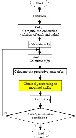
[image:4.595.356.487.463.700.2]

The flowchart of the proposed algorithm is given in Fig.2 and the flowchart of the modified εRDE algorithm is shown in Fig.3. In Fig.2, it is noted that the best individual is chosen as the estimation results ˆxk at each iteration.

Figure 2. The flowchart of proposed algorithm

suitable for iterative estimation, which can be expressed as

 

 

con

con

con

1

1 1 , 1

0, cp k

k T

k T

k T 



 _{  }

 _  _  

  _{ }



 

(27)

with ε(1) is the sum of the constraint violation degree of the top a-th individual and a=0.2Np is chosen in this paper.

Tcon and cp are constants.

[image:5.595.333.538.75.155.2] [image:5.595.94.286.99.145.2]

For (27), in the initial iteration stage a larger constraint violation is allowed. The individuals after evolution will approach the global optimum but not converge exactly to one point.

Figure 3. The flowchart of the modified εRDE algorithm In order to reduce the complexity of εRDE algorithm, the case of φ1=φ2 is not taken into consideration due to

the fact that it is of very small probability for φ1=φ2 in

practical applications. As a result, the ε rank comparison defined in [9] can be simplified as follows.



1 1

 

2 2



1 2 1 2 1 2

, ,

, ,

otherwise

f f

f  f    

 

 



  



 (28)



 



1 2 1 2

1 1 2 2

1 2

, ,

, ,

otherwise

f f

f  f    

 

 



  



 (29)

V. SIMULATION ANALYSES

A C/A signal of GPS is simulated assuming a scenario composed of a direct signal and two multipaths. The multipaths are in-phase, which is the worst possible case, which means Am k, m k, , m=0, 1, 2. The multipath

parameters are supposed to be unchanged during observation period. The system noise is assumed to be Gaussian noise with the mean being zero and the covariance matrix Q=diag(0.001*ones(1, 2(M+1)). The correlator number should be larger than or equal to the state dimension number, i.e., S≥D. In this simulation, set S=9 (ds=0.7Tc, 0.5Tc, 0.3Tc, 0.1Tc, 0, -0.1Tc, -0.3Tc, -0.5Tc,

-0.7Tc). The true values are set as A0=0.9, A1=0.6, A2=0.3,

l0=100Tc, l1=0.2Tc, l2=0.6Tc. Ts=Tc/10,lˆ0 100.2Tc. Our

goal is to estimate A0, A1, A2, l0, l1, l2.

The non-Gaussian measurement noise with Gaussian mixture PDF f=λ1N(μ1,₁2)+λ2N(μ2,₂2)is constructed for

simulation, where N(μ, σ2_{) is a Gaussian distribution with}

the mean μ and variance σ2_{. λ}

1 and λ2 are the weights

corresponding to the first Gaussian individual and the second Gaussian individual with λ1 +λ2=1. The simulation

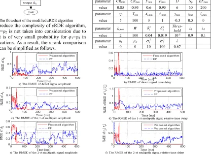
[image:5.595.97.248.232.467.2]

parameters are given in Table.1. TABLE.1

SIMULATION SETTING UNDER NON-GAUSSIAN NOISE parameter CRmin CRmax Fmin Fmax D Np EFmax

value 0.85 0.95 0.6 0.95 6 60 200

parameter cp Tcon Ai,min Ai,max γmin γmax li,min

value 5 100 0 1 -0.5 0.5 0

parameter li,max W

2 1

 2

2

 Thres-

hold λ1 λ2

value 2 100 0.04 0.019 10-5 _{0.9 0.1}

parameter μ1 μ2 12 2 2  λ

value 0 0 10 100 0.67

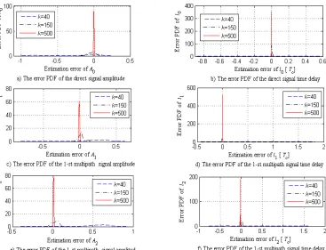
[image:5.595.115.543.437.752.2]

[image:6.595.116.483.73.354.2]

Figure 5. The error PDFs of the proposed algorithm

The comparisons between the proposed algorithm and a standard PF algorithm are shown in Fig.4. The same initial population is used for the proposed algorithm and PF. It can be seen the proposed algorithm has a better estimation accuracy and smaller randomness. To further inspect the performance of the proposed algorithm, the error PDF of the proposed algorithm is shown in Fig.5. We can observe that the error PDF of the proposed algorithm becomes more and more concentrated around zero mean as the iteration proceeds, which indicates the estimation error becomes narrower and the randomness of estimation error becomes smaller.

VI CONCLUSION

In this paper, a modified εRDE algorithm is proposed

to solve the two-multipath estimation problem in non-Gaussian noise. Compared with the previous work on multipath estimation, the contributions of this paper are two folds: (1) two- multipath case is considered; (2) the multipath problem is solved as an optimization problem with CEEC as its objective, the second-order moment of estimation error and the prior information being considered as the constraints. A εRDE algorithm is modified to solve the formulated problem. The simulation results verified the effectiveness of the proposed algorithm for two-multipath estimation. At the current stage, only the static multipath is considered and the proposed algorithm appears to be more time consuming compared with the PF algorithm. These issues will be further investigated in the future work.

REFERENCES

[1] E. S. Lohan, R. Hamila, A Lakhzouri, M. Renfors, “Highly efficient techniques for mitigation the effects of multipath propagation in DS-CDMA delay estimation,” IEEE Transactions on Wireless Communication, vol.4, no. 1, pp. 149-162, Jan. 2005.

[2] C. Pau, F. P. Carles, “A Bayesian approach to multipath mitigation in GNSS receivers,” IEEE Journal of Selected Topics in Signal Processing, vol. 3, no. 4, pp. 695-706, 2009. [3] B. R. Townsend, P. C. Fenton, K. J. Van Dierendonck, et al,

“Performance evaluation of the multipath estimating delay lock loop,” Navigation, vol. 42, no. 3, pp. 503-514, Jan. 1995.

[4] R. A. Iltis. “Joint Estimation of PN Code Delay and Multipath Using the Extend Kalman Filter,” IEEE Transactions on Communication, vol. 38, no. 10, pp. 1677-1685, 1990.

[5] L. Cheng, M. F. Ren, G. Xie, “Multipath estimation based on centered error entropy criterion for non-Gaussian Noise,”

IEEE Access, DOI: 10.1109/ACCESS.2016.2639049, 2016. [6] C. Shannon, W. Weaver, “The mathematical theory of

communication”, University of Illinois Press, Urbana, 1949. [7] Y. Liu, H. Wang, C. H. Hou, “UKF based nonlinear filtering using minimum entropy criterion,” IEEE Transaction on Signal Processing, vol. 61, no.20, pp. 4988-4999, Oct. 2013. [8] W. F. Liu, P. P. Puskal, J. C. Principle. “Correntropy: properties and applications in non-Gaussian signal processing,” IEEE Transaction on Signal Processing, vol. 55, no.11, pp. 5286- pp.5298, Nov. 2007.

[9] T. Takahama, S. Sakai. “Efficient constrained optimization by the ε constrained rank-based differential evolution,”