City, University of London Institutional Repository
Citation
: Argasinski, K. & Broom, M. (2017). Evolutionary stability under limited
population growth: Eco-evolutionary feedbacks and replicator dynamics. Ecological
Complexity, doi: 10.1016/j.ecocom.2017.04.002
This is the accepted version of the paper.
This version of the publication may differ from the final published
version.
Permanent repository link:
http://openaccess.city.ac.uk/18115/
Link to published version
: http://dx.doi.org/10.1016/j.ecocom.2017.04.002
Copyright and reuse:
City Research Online aims to make research
outputs of City, University of London available to a wider audience.
Copyright and Moral Rights remain with the author(s) and/or copyright
holders. URLs from City Research Online may be freely distributed and
linked to.
City Research Online: http://openaccess.city.ac.uk/ [email protected]
Evolutionary stability under limited population growth:
1
Eco-evolutionary feedbacks and replicator dynamics.
2
K. Argasinski* 3
Department of Mathematics, University of Sussex, 4
Brighton BN1 9QH, UK. 5
[email protected], tel. 012 73877345 6
M. Broom 7
Department of Mathematics, City, University of London, 8
Northampton Square, London EC1V 0HB, UK. 9
Abstract
12
This paper further develops a new way of modelling evolutionary game mod-13
els with an emphasis on ecological realism, concerned with how ecological factors 14
determine payo¤s in evolutionary games. Our paper is focused on the impact of 15
strategically neutral growth limiting factors and background …tness components 16
on game dynamics and the form of the stability conditions for the rest points 17
constituted by the intersections of the frequency and density nullclines. It is 18
shown that for the density dependent case, that at the stationary state, the 19
turnover coe¢ cients (numbers of newborns per single dead adult) are equal for 20
all strategies. In addition, the paper contains a derivation of the EESS (eco-21
evolutionarily stable states) conditions, describing evolutionary stability under 22
limited population growth. We show that evolutionary stability depends on the 23
local geometry (slopes) of the intersecting nullclines. The paper contains exam-24
ples showing that density dependence induces behaviour which is not compatible 25
with purely frequency dependent static game theoretic ESS stability conditions. 26
We show that with the addition of density dependence, stable states can become 27
unstable and unstable states can be stabilised. The stability or instability of 28
the rest points can be explained by a mechanism of eco-evolutionary feedback. 29
1
Introduction
30
Current developments in evolutionary biology emphasize the role of relationships 31
2011, Pelletier.et al. 2009). This perspective is very interesting from the point 33
of view of formal modelling, which can contribute to this research program not 34
only by quantitative predictions, but also by rigorous conceptualization of the 35
analyzed mechanisms. Thus, this direction should also be considered in the 36
development of modelling approaches such as evolutionary game theory. Recent 37
developments in this …eld, focused on the realistic modelling of the turnover of 38
individuals (i.e. the dynamics of the replacement of the dying adult individuals 39
by newly introduced juveniles), can be useful in pursuing this goal. In this study 40
we will analyze the interplay between selection dynamics of strategy frequencies 41
and the ecological dynamics shaping the population size. In addition we will 42
investigate the relationships between game theoretic equilibrium conditions and 43
nullclines of the selection and ecological dynamics. 44
In the classical approach to evolutionary game theory (Maynard Smith 1982,
Hofbauer and Sigmund 1988, 1998), a well-mixed population with clonal
repro-duction and no mutation evolves under natural selection. The strategies are
heritable phenotypic traits or di¤erent behavioral patterns and payo¤ functions
describing their …tness. The merits and limitations of such an approach are
discussed in Maynard Smith (1982) (for interesting general work based upon
similar principles but with an in…nite strategy set, see for example Gorban,
2007; Meszena et al., 2006; Oesschler and Riedel, 2001). An abstract “…tness”
is expressed as an in…nitesimal growth raterand described in unde…ned “units”,
which are the currency in which evolutionary “costs”and “bene…ts”are counted.
dynamics, de…ned on thek 1dimensional simplex. Thenqi=ni=Pjnj (niis
the number of carriers of thei-th strategy) is the frequency of thei-th strategy
andri(q)is its payo¤ function:
_
qi=qi
0 @ri(q)
X
j rj(q)
1
A for i= 1; : : : ; k 1: (1)
In the classical approach to evolutionary game modelling there is no explicit 45
analysis of the impact of limitations of the population size. In more complex 46
approaches (Cressman 1992, Cressman et al 2001, Cressman and Garay 2003, 47
Argasinski 2006) density dependence has been taken into consideration. The 48
speci…c case of selectively neutral density dependence, which means that the 49
growth suppression acts on all strategies in the same way, was analyzed in 50
Argasinski and Koz÷owski (2008). It was shown there that the classical approach 51
(1) can be problematic, when growth limitation, related to the logistic equation, 52
is implemented. The dynamics stop when the carrying capacity is reached. This 53
is caused by the fact that both birth and death rates are suppressed, leading 54
to a population of immortal individuals. This problem can be solved by using 55
the assumption that only the birth rate is suppressed by juvenile recruitment 56
survival, which leads to a generalization of the replicator dynamics completed 57
by the equation for the population size (Argasinski and Broom, 2012). In this 58
approach payo¤s are described explicitly as demographic vital rates (mortality 59
and fertility), not as an abstract …tness. Thus assume thatWi(q)is the fertility 60
function, suppressed by the density dependent juvenile recruitment function 61
(1 n=K) (where n = Pjnj and K is the carrying capacity describing the 62
This leads to the following: 64
_
qi = qi
2 4
0
@Wi(q) X
j
Wj(q)
1
A 1 n
K
0
@di(q) X
j dj(q)
1 A 3
5 for i= 1; : : : ; k (2)1:
_
n = n
0
@ 1 n
K
X
j
Wj(q) X
j dj(q)
1
A; (3)
65
where the bracketed term from (1) splits into two brackets describing di¤er-66
ences in fertilities and mortalities. The replicator system (2) is completed by 67
equation (3) describing the changes of the population size caused by selection of 68
the strategies. A similar method was applied in a number of papers (Hauert et 69
al., 2006; Hauert et al., 2008; Argasinski and Koz÷owski, 2008; Zhang and Hui, 70
2011; Argasinski and Broom, 2012; Huang et al., 2015; Gokhale and Hauert, 71
2016). In this approach population size does not converge to an arbitrary car-72
rying capacity as in many models (for example Cressman and Krivan, 2010; 73
Krivan, 2013) but to a dynamic equilibrium between mortality and fertility 74
(this is often called an emergent carrying capacity, Bowers et al., 2003; Sieber 75
et al., 2014). The general selective properties of this approach were presented in 76
Argasinski and Broom (2013), where the simpli…ed version of (2,3) with payo¤s 77
as constants was analyzed. It was shown there that when the population reaches 78
the close neighbourhood of the population size equilibrium (nullcline of the equa-79
tions forn), then newborns form the pool of candidates from which individuals 80
replacing the dead adults in their nest sites will be drawn. This mechanism 81
maximize the number of newborns replacing each single dying adult (termed 83
"turnover coe¢ cient"), however among strategies maximizing this quantity it is 84
pro…table to maximize the mortality (the number of dead adults) and thus also 85
the number of newborns replacing them. Therefore, we have a two stage …tness 86
measure. 87
The previous paper, Argasinski and Broom (2012), was focused on the de-88
scription of the above approach using demographic parameters, mortality as the 89
probability of death (or equivalently survival) and fertility as per capita number 90
of o¤spring. This allows for a description of the abstract and unclear parame-91
ters such as “…tness” or “growth rate” by clear and measurable parameters. In 92
addition, the new approach is focused on the detailed description of the struc-93
ture of cause-e¤ect chains underlying the particular interactions. For example, 94
the modelled interaction described by the game theoretic structure can be com-95
posed of several mortality and fertility stages following each other. This aspect 96
can be illustrated by the simplest case of a single pre-reproductive mortality 97
stage preceding the fertility stage. Then only survivors of the interaction can 98
reproduce, which should be incorporated into the payo¤ functions. Thus the 99
fertility payo¤sWi(q)will be replaced by the mortality-fertility trade-o¤
func-100
tionVi(q) =Pjqjsi(ej)Wi(ej)(whereej is the vector describing thej-th pure
101
strategy) describing the reproductive success of the survivors. The new concep-102
tual framework was applied to the classical Hawk-Dove game to illustrate the 103
The general framework was clari…ed in a second paper (Argasinski and 105
Broom, submitted) focused on the derivation of the game theoretic model from 106
the general population dynamics model also describing factors other than the 107
modelled type of interaction. For example individuals playing the Hawk-Dove 108
game during the mating con‡ict (the modelled focal interaction) can also be 109
killed by predators (background interactions without relation to the strategies 110
in the focal game). This leads to a model of a population of individuals playing 111
di¤erent types of games describing di¤erent interactions occurring at di¤erent 112
rates (see Appendix 1 for more details). Thus, by analogy with chemical kinetics 113
(Upadhyay, 2006), the game theoretic structure is equivalent to stoichiometric 114
coe¢ cients describing the outcomes of a single reaction between particles (in our 115
case, interactions between individuals) and the rate of occurrence is equivalent 116
to the reaction rate. The new framework focuses on births and deaths (described 117
by separate payo¤ functions) as the aggregated outcomes of the physical inter-118
actions between individuals and the elements of the environment. This is why 119
it was described as the “event-based approach” in the previous papers. This 120
approach is focused on the development of the mechanistic interpretations of the 121
theoretical notions which was emphasized by Geritz and Kisdi (2012). However, 122
in game theoretic analysis we are interested in one particular type of interac-123
tion referred as a focal game (or a few chosen types a¤ected by an analyzed 124
phenotypic trait in a more general case) while the aggregated outcomes of the 125
other games will constitute the background …tness. In e¤ect (3) should be com-126
(see Appendix 1 for details). In addition, the“nest site lottery” operates not 128
only on the demographic outcomes of the modelled game, but on outcomes of 129
all interactions, which means that the aggregated fertility outcomes of events 130
constituting the background …tness (other games played by individuals) are also 131
the subject of this mechanism. 132
The values of the background payo¤s can seriously a¤ect the game dynam-133
ics as shown in Argasinski and Broom (submitted). In Argasinski and Broom 134
(2012) it was also shown that under the in‡uence of neutral density dependence, 135
the behaviour of the system is di¤erent from that in the model with unlimited 136
growth. The main di¤erence is that in the model with unlimited growth there 137
are only equations describing the evolution of strategy frequencies, while in the 138
density dependent model there is an additional equation describing the size of 139
the population and fertilities are a¤ected by juvenile mortality described by 140
logistic suppression. In e¤ect, in the density dependent model, the stable fre-141
quency becomes a function ofndescribing the nullcline constituting the manifold 142
of game theoretic Nash equilibria (population states with equal growth rates for 143
all strategies). In addition, the equation for the population size leads to another 144
nullcline being a function of the population composition and is a¤ected by back-145
ground payo¤s. This nullcline has a very important biological meaning since it 146
describes the ecological equilibria, conditional on the current strategic compo-147
sition. In the game theoretic literature it is often referred as the stationary 148
density surface (Cressman et al., 2001; Cressman and Garay, 2003a; Cressman 149
nullclines, which can be stable or unstable. 151
The density and frequency nullclines describing the ecological and game 152
theoretic equilibria are important for the mechanistic interpretation of the phe-153
nomenon in terms of feedbacks. New phenomena can emerge, for example the 154
existence of a stable pure Hawk solution in addition to the stable mixed equilib-155
rium (Argasinski and Broom, 2012). The additional stable rest point is caused 156
by neutral density dependence. This paper contains a general analysis of system 157
stability and a mechanistic explanation of the interplay between the conver-158
gence to the selection equilibrium describing the stable population composition 159
(described by the frequency nullcline) and the convergence to the ecological 160
equilibrium describing the stable population size (described by the density null-161
cline). The study shows when the stability is fully determined by the behaviour 162
along the nullclines and the problem can be reduced to the static game theo-163
retic analysis limited to simple algebraic inequalities, and when the full dynamic 164
model involving di¤erential equations should be applied. 165
2
Results
166
2.1
Selectively neutral density dependence and the
con-167
cept of eco-evolutionary feedback
168
Now let us focus on the impact of selectively neutral density dependence act-169
Broom (2012) is a case where there is a single equation for strategy frequen-171
cies, and the space of the population composition is the unit interval. We are 172
interested in the rest points of the system and their stability. Since we have a 173
system of two equations, one onq and one on n, we can expect two nullclines 174
obtained by calculation of the zero points of the equations. 175
2.2
General form of the analyzed models
176
Argasinski and Broom (2012) contains the derivation of both attracting null-177
clines for frequency, and density equations (described below) for the Hawk-Dove 178
example, and the calculation of their intersections. However, a rigorous stabil-179
ity analysis was limited to the case when the system is in ecological equilibrium 180
(Theorem 2 of that paper). In this paper we carry out the analysis of the gen-181
eral stability conditions free from this restriction, …nd some surprising results, 182
and demonstrate that the previous analysis is insu¢ cient to fully explain the 183
behaviour of the system in some cases. 184
In this section we start from the general dynamical system for two strategies 185
from Argasinski and Broom (2012). Assume thatq= (q1;1 q1)is the vector of
186
frequencies describing the strategic composition of the population. ThenVi(q)
187
and si(q) = 1 di(q) describe the fertility and adult survival payo¤s related
188
to the focal interactions, being the subject of game theoretical analysis. The 189
logistic coe¢ cient 1 Kn describes the density dependent juvenile survival 190
and background fertility and mortality describe the impact of other factors 191
to the following general set of equations: 193
_
q1=q1 0 @(V1(q)
X
j
qjVj(q)) 1 n
K + (s1(q)
X
j
qjsj(q))
1 A; (4)
_
n=n
+X
i
qiVi(q)
!
1 n
K +
X
i
qisi(q) 1
!
; (5)
see Appendix 1 for a detailed derivation and description of possible speci…c
modelling approaches that can be considered with the above general
frame-work). Thenq~(n)is the nullcline of equation (4),n~(q)is the nullcline of
equa-tion (5) and their intersecequa-tion is the point (^n;q^). To analyse the underlying
dynamics, the above system can be presented in the most general form
with-out the distinction between focal interactions, described by game payo¤s, and
the background fertility and mortality rates. Then the system (4,5) can be
denoted in terms of general birth and death rates, B1(q) = V1(q) + 0
and M1(q) = 1 s1(q) + 0 (since fecundities and mortalities are always
non-negative) describing the demographic outcomes of all interactions
(includ-ing focal game payo¤s and background payo¤s and respectively). Then
B(q) = qB1(q) + (1 q)B2(q) 0 and M(q) = qM1(q) + (1 q)M2(q) 0
are the mean general fecundity and mortality, respectively. This leads to the
system:
_
q1=g(n; q) =q1 B1(q) B(q) 1
n
K M1(q) M(q) ; (6)
_
n=f(n; q) =n B(q) 1 n
where equation (6) is written focusing on the …rst strategy; an analogous equa-194
tion would denote the frequency of the second strategy. We will also use the 195
auxiliary terms (as we see in the associated appendices),ru(q) =B(q) M(q)
196
which is the rate of unsuppressed growth and L = B(q)=M(q) which is the 197
turnover coe¢ cient. 198
2.3
Properties of the stationary points related to the turnover
199
of individuals
200
In many modelsq~(n)andn~(q)de…ned as the respective nullclines will exist (in 201
some cases they will be attracting nullclines). Expressingq as a function ofn
202
(according to the implicit function theorem), the nullcline q~(n) is de…ned by 203
the value of q for which g(n; q) = 0 (the right-hand side of equation (6) is 0 204
for any givenn). It is possible that there is more than one such solution, and 205
so more than one such nullcline. Similarly, expressingn as a function of qfor 206
f(n; q) = 0, the nullcline ~n(q)is de…ned by the value ofnfor which the
right-207
hand side of equation (7) is 0 for any givenq. The nullclines, representing the 208
equilibria of interplaying processes (strategic selection and convergence to the 209
ecological equilibrium) will play important roles in the derivation of the static 210
game theoretic conditions (the inequalities for payo¤s of the strategies that 211
should be satis…ed for evolutionary stability). Those conditions will extend the 212
classical ESS concept to the ecological concept. In addition, on the nullcline 213
representing the equilibria of one process, the dynamics is determined by the 214
by game dynamics only. The question arises, when can the behaviour of the 216
complicated dynamical system be described by a set of algebraic inequalities? 217
Now let us analyze the properties of the stationary points of systems of 218
this type. In classical evolutionary game theory, at the stationary points (a 219
Nash equilibria) there is equality of …tness among all strategies present in the 220
population; we note that this property becomes trivial after the addition of 221
density dependence since all growth rates are equal to zero at the stationary 222
states. The new framework presented here is de…ned with respect to fertility 223
and mortality separately. Thus the question arises: is there a characterization 224
of the stationary points in the new theory equivalent to the equality of …tness 225
in classical theory? Here the notion of the turnover coe¢ cient Bi(q)=Mi(q), 226
describing the number of newborn candidates replacing a single dead individual, 227
should be recalled. The name “turnover coe¢ cient”was introduced, and the 228
properties of this term were analyzed, in Argasinski and Broom (2013). Similar 229
notions can be found in older papers, for example in Rosenzweig and MacArthur 230
(1963) and Cheng (1981), and an analogous notion describing the ratio of energy 231
allocated to reproduction to mortality can be found in papers related to life 232
history theory (Taylor and Williams, 1984; Koz÷owski, 1992 and 1996; Werner 233
and Anholt, 1993; Perrin and Sibly, 1993; for an overview see Koz÷owski, 2006). 234
The turnover coe¢ cient can be useful for the characterization of the stationary 235
points of the dynamics even in the general case ofkstrategies (not only two as 236
Theorem 1
238
Any intersection of the nullclines is an equilibrium point, and at such an 239
intersection: 240
a) The turnover coe¢ cients of all strategies are equal:
Bi(q)
Mi(q)
= Bj(q)
Mj(q)
= B(q)
M(q): (8)
b) The focal game-speci…c demographic payo¤s Vi(q)and si(q) satisfy the 241
following condition 242
Vi(q) M(q)
B(q) (1 si(q)) =Vj(q)
M(q)
B(q) (1 sj(q)): (9)
243
For a proof see Appendix 2. 244
Condition b) can be interpreted as equality of the suppressed Malthusian 245
growth rates related to the focal game (and one divided by the population 246
average turnover coe¢ cient M(q)=B(q) = (1 s(q) + )=(V(q) + ) is the 247
density dependent juvenile recruitment survival probability). Note that this 248
property should be satis…ed in general for any number of strategies. 249
Corollary 1
250
If the focal game-speci…c turnover coe¢ cients satisfy
Vi(q)
(1 si(q)) =
Vj(q)
(1 sj(q)) =
B(q)
M(q); (10)
Thus the condition of equality of the turnover coe¢ cients can be extended on 252
the focal game payo¤ functions, but it is not general. We can imagine stationary 253
points where point b) from Theorem 1 is satis…ed but there are no equality of 254
the focal game turnover coe¢ cients. A question arises about the stability of 255
the stationary points where all strategies have equal turnover coe¢ cient. For 256
the general case this can be very complex, thus we start from the basic models 257
and focus on the stability of the stationary states for two competing strategies. 258
Consider the phase spaceq n, consisting of all possible values ofqandn. On 259
the nullclines q~(n) and n~(q) the right-hand side of the equations (6) and (7) 260
respectively equals zero, and these nullclines divide the phase space into regions 261
of growth and decline forqandn. When the right-hand side of equation (6) is 262
negative we have thatq >q~(n)is the region of decline forq. 263
We note that in the method of static game theoretic analysis presented in 264
Argasinski and Broom (2012), the attractor population size n~(q) was substi-265
tuted into the right hand side of equation (6). Substitution ofn~(q) into q~(n)
266
leads to the inequalityq <(>)~q(~n)describing the regions of growth (decline) 267
of q lying on the density nullcline ~n(q). In Argasinski and Broom (2012) the 268
inequality q q~(~n) has the form of a quadratic equation (see Theorem 2 and 269
Appendix 5 there). Zeros of this equation are intersections of the density and 270
frequency attracting nullclines. Thus under the assumption of ecological equi-271
librium, this method shows which intersection is stable and unstable. This is 272
a rigorous analysis but it is strictly limited to the attracting density nullcline. 273
of the attracting density nullcline? There are relationships between the density 275
and frequency nullclines, but these cannot necessarily be extrapolated to the 276
general neighbourhood of their intersections. This is summarized by technical 277
Lemma 1 below, where we assume the standard notation for partial derivatives 278
gq =@g=@q,gn =@g=@n, fq =@f =@q and fn =@f =@n of the right hand sides 279
of equations(6,7). 280
Lemma 1
281
Assume that the attracting density nullcline and frequency nullcline exist 282
and they intersect. Then: 283
a) if gq(n;q~(n)) < 0 (the frequency nullcline is an attractor of the frequency
284
dynamics) then if the intersection is stable (unstable) on the density nullcline, 285
it is stable (unstable) on the frequency nullcline. 286
b) if gq(n;q~(n)) > 0 (the frequency nullcline is a repeller of the frequency 287
dynamics) then if the intersection is stable (unstable) on the density nullcline, 288
it is unstable (stable) on the frequency nullcline. 289
For a proof see Appendix 3. 290
Thus in the case when the frequency nullcline is the attractor of the frequency 291
dynamics, which implies that in the density independent case it will be a stable 292
rest point, stability on the attracting density nullcline can be extrapolated to the 293
attracting frequency nullcline. This property can be useful for the derivation 294
of the static conditions for Eco-Evolutionary stability. Part b) of Lemma 1 295
case of an unstable frequency nullcline the selection process and the ecological 297
process will always act antagonistically. If one process will lead to stabilization 298
of the rest point the second process will act towards destabilization. Thus 299
we need some additional criteria describing this antagonistic relationship. The 300
potential complexity of behaviour will be shown by numerical examples in the 301
next section. 302
2.4
Numerical examples and their analysis
303
This section contains numerical simulations of the updated Hawk-Dove game 304
(52,53) (see Appendix 4 for details) to show the dynamics induced by the 305
eco-evolutionary feedback mechanism. For simplicity we set the background 306
fertility to be equal to zero. In Theorem 2 in Argasinski and Broom (2012) 307
the local stability of intersections on the stable density nullcline for the Hawk-308
Dove game was analyzed. However the trajectories of the population away from 309
this nullcline prior to convergence are also interesting and will have ecological 310
interpretations. In Argasinski and Broom (2012) numerical simulations showed 311
the interplay between selection dynamics and the dynamics of the population 312
size. It was shown that ecological dynamics can seriously a¤ect the rules of 313
the game while frequency dynamics determine the population size. This was 314
mechanistically explained in that paper by the impact of density dependent 315
juvenile mortality. In this section we will focus on the relationship between 316
the trajectories, population size and the geometry of the attracting nullclines 317
~
Argasinski and Broom (2012). 319
FIGURE 1 HERE 320
FIGURE 2 HERE 321
FIGURE 3 HERE 322
FIGURE 4 HERE 323
In Argasinski and Broom (2012) results of the numerical simulations em-324
phasized the role of the intersections of both nullclines. In this paper we want 325
to show the trajectories prior to convergence. To emphasize the role of both 326
nullclines, in Figures 1-4, model parameters are chosen to set both intersections 327
at values of frequenciesqclose to 0 and 1. This allows us to maximize the area 328
falling between the nullclines which are very close to each other in the cases 329
when intersections are relatively close (see for example Figure 4). Some of the 330
numerical simulations support the intuition that the dynamics converge to the 331
close neighbourhood of the attracting density nullcline and then trace the equi-332
librium size value (Figure 1). In this case the assumption from Argasinski and 333
Broom (2012) of the population taking the stable size for a given frequency is 334
justi…ed. 335
However, this happens when both nullclines are placed at relatively high 336
densities. At lower densities the trajectory does not reach a strict neighbour-337
hood of the attracting density nullcline (Figure 2), but converges to a surface 338
lying between the frequency and density nullclines. At very low densities the 339
attracting nullcline (Figure 3). We note that this e¤ect is suppressed by pop-341
ulation growth. In some cases the attracting nullcline is located in the close 342
neighbourhood of the frequency attracting nullcline and traces it nearly to the 343
equilibrium (Figure 4). Thus, the assumption that frequency selection occurs 344
on the attracting density nullcline can sometimes be seriously wrong. In the 345
general case the geometry of both nullclines plays an important role in the dy-346
namics and what happens in the region limited by those surfaces is crucial. At 347
higher densities there is a stronger convergence towards the attracting density 348
nullcline while at lower densities there is a stronger attraction towards the fre-349
quency attracting nullcline. Therefore, the ecological equilibrium assumption is 350
a simpli…cation of the full problem. In addition, on all …gures we can observe 351
the clearly visible convergence of the trajectories to the unique invariant man-352
ifold. However, the behaviour on these manifolds seems to be compatible with 353
the projection of the vector …eld on the nullcline n~(q) (and also by Lemma 1 354
on the nullcline q~(n)). This suggests that the stability of the intersection can 355
be described by a simple set of algebraic equations, which will constitute the 356
Eco-Evolutionary static analysis. 357
Note that in the above examples the attracting frequency nullcline represents 358
the set of game theoretic Nash equilibria, conditional on the actual ecological 359
conditions represented by juvenile mortality, determined by population size. 360
However, we have two types of intersection representing the stationary points. 361
One is stable, thus it is compatible with the underlying purely game theoretic 362
equilibrium in the density independent case can be destabilized by ecological 364
factors. However, we can imagine the opposite situation, where the intersection 365
of the repelling frequency nullcline (representing the set of invasion barriers con-366
ditional on the actual population size) can be stabilized by the impact of density 367
dependence. This is illustrated by the following phenomenological example: 368
Example 1: the stabilization of a stationary point by density
de-369
pendent pressure in case of the repelling frequency nullcline. 370
Assume that there are two strategies, where the functions
B1(q) =
2
3q
2+2
3q andM1(q) =
7 9
q
3
are the fertility and mortality of the …rst strategy, while
B2(q) =
2
3q
2andM 2(q) =
4 9
q
3
are those of the second. This leads to the following replicator equation (see
Appendix 5 for detailed derivation):
_
q= q
3(1 q) ((2q 1)); (11)
whereq = 1=2 is the unstable rest point (invasion barrier). However when we 371
extend this model to the density dependent case, the situation is di¤erent. We 372
obtain: 373
_
q = q
3(1 q) (2q(1 n=K) 1); (12)
_
n = 4
3n q
2(1 n=K) 1
3 : (13)
Calculation of the frequency and density nullclines gives: 374
~
q= 1
2(1 n=K) andn~ = 1
1
3q2 K.
375
Thus on the density nullcline juvenile mortality is1 ~n=K= 1=3q2, leading 377
to the stationary state q^ = 2=3 and the respective population size n^ = K=4
378
(juvenile mortality is 1 n=K^ = 3=4). This example clearly shows that the 379
frequency nullcline need not be attracting for the stability of the respective in-380
tersection with the attracting density nullcline to hold (see Figure 5). 381
FIGURE 5 HERE 382
In this case there is no convergence of the trajectories to the unique manifold. 383
Figure 5 shows that in the neighbourhood of the nullclines there is a spiral at-384
traction to the intersection. However, below the nullclines there is a huge region 385
of extinction and convergence to the frequency 0. This pattern is caused by the 386
fact that at low densities pressure from the frequency dynamics is stronger than 387
that from the density dynamics. Thus at low population sizes, the frequency 388
nullcline acts as the invasion barrier as in the case of unlimited growth. How-389
ever, this is caused by the decrease of the population size induced by the density 390
dynamics. This leads to an emergence of the additional boundary between the 391
basins of attraction. This boundary cannot be justi…ed by any existing condition 392
for evolutionary stability. Thus the dynamics can produce patterns that cannot 393
be classi…ed by known static ESS notions, and in this case the full analysis of 394
2.5
General stability conditions
396
The examples presented above suggest the necessity of a general stability
analy-sis. This will enable extrapolation of the stability analysis of the Hawk-Dove
example from Argasinski and Broom (2012) to the general neighbourhood of
the intersection, not limited to the attracting density nullcline. Coordinates
of the intersection are(^n;q^). Stability along the attracting density nullcline is
described by the directional derivative (a total derivative expressed in terms of
our four partial derivatives)
dg(~n(q); q)
dq =gq(^n;q^) gn(^n;q^)
fq(^n;q^)
fn(^n;q^)
: (14)
397
Below, by application of standard linearization methods we will derive the 398
general stability conditions for intersections of the nullclines: 399
Theorem 2
400
If for the system described by equations (6) and (7), nullclinesq~(n)andn~(q)
401
exist, then: 402
The intersection is stable if the following EESS (Eco-Evolutionarily Stable
State) conditions are satis…ed:
a)
gq(^n;q^)<jfn(^n;q^)j; (15)
b)
dg(~n(q); q)
403
For a proof see Appendix 6. 404
A question arises about the interpretation of the above stability conditions. 405
Condition a) means that attraction to the density nullcline is stronger than 406
repellence from the frequency nullcline. This means that in the antagonistic 407
relationship between selection and the ecological process indicated by point b) 408
of Lemma 1, the stabilizing ecological process should be stronger. If the null-409
clineq~(n)is attracting (which means that it consists of stable Nash equilibria) 410
then condition a) is satis…ed automatically. Condition b) is equivalent to sta-411
bility along the density nullcline n~(q). Thus for the attracting nullcline q~(n)
412
the stability of the global equilibrium is equivalent to the behaviour along the 413
nullclinen~(q). This justi…es the static ESS analysis based on the substitution of 414
the ecological equilibriumn~(q)to the dynamics and the analysis of signs of the 415
right hand sides of theq equations as in Theorem 2 in Argasinski and Broom 416
(2012). Note that, according to Lemma 1, condition b) implies instability on 417
the repelling nullcline q~(n), representing the game theoretic invasion barriers. 418
However, in this case, if the attraction towards nullclinen~(q) is stronger than 419
the repellence from nullcline q~(n), then the intersection can be stable despite 420
this. Note that for the intersection of the repelling frequency nullcline and den-421
sity nullcline from Example 1, both conditions are satis…ed (see Appendix 7 422
for the detailed calculations). According to Lemma 1, satisfying condition b) 423
clineq~(n) and repellence if the frequency nullclineq~(n)is repelling. Example 425
1 supports the results from Lemma 1. The projection of the ‡ow orthogonal 426
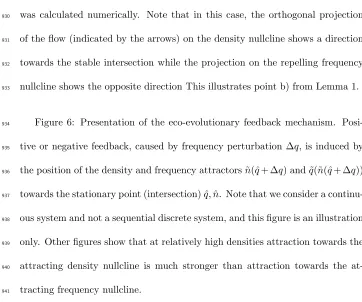
to the density nullcline (see arrows on Figure 6) shows that it will be stable, 427
while on the frequency nullcline it will be unstable. However the general spiral 428
dynamics cannot be reduced to convergence along one of the nullclines. 429
Note that the ‡ow is horizontal on the frequency nullcline and vertical on the
density nullcline. Thus the orthogonal projection of the ‡ow is determined by
the slope of the respective nullcline. We shall assume that in the neighbourhood
of the intersection functionsg andf are locally invertible, so that there is a
1-1 correspondence between n and q, at least in the vicinity of a root. This
will be true for essentially any biological system, as situations where this is
not so, corresponding to nullclines slopes with zero or in…nite gradient, are
examples of so-callednon-generic games, see e.g. Broom and Rychtar, 2013). This means that both stability conditions can be interpreted in terms of slopes
of the nullclines. The slope of the frequency nullcline is
Uq=
dg(g 1(0;q^);q^)
dq ; (17)
and the slope of the size nullcline is
Un=
df(f 1(0;q^);q^)
dq : (18)
Then the above conditions are equivalent to the following lemma: 430
Lemma 2
Provided that the inverses from equations (17) and (18) exist, Condition 432
a) from Theorem 2 is clearly satis…ed whengq(^n;q^) 0. For gq(^n;q^)>0, we
433
require the following condition to be satis…ed: 434
gn(^n;q^)is negative (positive) and :
Uq<(>)
^
n
^
q B1(^q)=B(^q) 1
: (19)
435
Condition b) is satis…ed whengn(^n;q^)is negative (positive) and: 436
Un >(<)Uq: (20)
437
For a proof see Appendix 8. 438
Note that the right hand side of the condition (19) depends only upon the 439
fertility stage; the mortality payo¤s are not present there. 440
2.6
Game theoretic notions revealed by dynamic stability
441
conditions
442
Now let us take the game theoretic perspective and analyze the above statements 443
from the strategic point of view. To do this we should describe the above 444
conditions in terms of general payo¤ functions explicitly and then we should 445
extract the focal game payo¤s from the background payo¤s in the conditions 446
De…nition 1: The semi-elasticity of the function f(x)at pointxis
df(x)=dx
f(x) ; (21)
which describes the change inf(x)scaled by its absolute value. 448
This concept can be generalized to the case of convex combination of func-449
tionsPqifi(x), as follows. 450
De…nition 2: The partial semi-elasticity of the functionfi(x)with respect
toPqifi(x)at point xis
dfi(x)=dx
P
qifi(x); (22)
which describes the equivalent scaled change in Pqifi(x) caused by the
451
componentfi(x). 452
Now we can derive the general stability conditions for the dynamics in the 453
form (6,7) expressed in terms of general demographic payo¤s. This is done in 454
the following theorem 455
Theorem 3
456
Condition a) has the form:
^
q B
0
1(^q) B0(^q)
B(^q)
M0
1(^q) M0(^q)
M(^q)
!
< B(^q)
M(^q) 1; (23)
where B(^q)
M(^q) 1describes the reproductive surplus, following De…nition 1,
B0(^q)
B(^q)
457
is the semi-elasticity ofBand following De…nition 2, B
0
1(^q)
B(^q) is the partial
semi-458
elasticity of B with respect to B1 (for mortalities M1(^q) and M(^q) we have
459
Condition b) is satis…ed when the semielasticities in payo¤s satisfy the
fol-lowing condition:
B0
1(^q)
B1(^q)
B0(^q)
B(^q)
M0
1(^q)
M1(^q)
M0(^q)
M(^q) <0: (24)
where B10(^q)
B1(^q)
is the semi-elasticity ofB1(similarly forM1).
461
For a proof see Appendix 9. 462
Note that both conditions resemble the bracket structure of the right hand
side of the replicator equations, or rather derivatives of it. The di¤erence is
that both conditions are expressed in terms of elasticities and partial
semi-elasticities instead of standard derivatives of payo¤ functions. The above
con-ditions are not expressed with respect to the focal games payo¤s. Thus they
should be extracted from general payo¤sB1(^q)andM1(^q). In e¤ect we obtain:
B1(q) =V1+ 0 andM1(q) = 1 s1+ , so that inequalities (23) and (24)
become
^
q V
0
1(^q) V0(^q)
V(^q) + + (s0
1(^q) s0(^q))
1 s(^q) +
!
< V(^q) +
1 s(^q) + 1 (25)
and
V0
1(^q)
V1(^q) +
V0(^q)
V(^q) + +
s0
1(^q)
1 s1(^q) +
s0(^q)
1 s(^q) + <0: (26)
Since the background payo¤s and do not depend on the traits under 463
consideration they should not depend on the frequency of the strategies in the 464
focal games. In e¤ect they vanish from the derivatives of the general growth 465
the stability in the particular focal type of interaction is determined by the 467
impact of other activities. Since = WB, = mB where describes the
468
average number of background events between two focal events, and WB and
469
mB are average background events fertility and mortality, parameters and
470
have a clear interpretation in the purely staticESS models too. This result 471
can be important for the research on animal personalities (Dall et al., 2004; 472
Wolf et al., 2007; Wolf and Weissing, 2010; Wolf and Weissing, 2012; Wolf and 473
McNamara, 2012). 474
The above results seriously alter our understanding of the self-regulation 475
mechanism in evolving populations showing the role of density dependent growth 476
limiting factors. They also suggest the relationship between the ESS approach 477
and some concepts already present in the debate on evolutionary ecology. We 478
can mechanistically interpret the stable and unstable intersections in terms 479
of eco-evolutionary feedback (Post and Palkovacs, 2009; Kokko and López-480
Sepulcre, 2007). 481
In the game theoretic framework this concept can be found in Argasin-482
ski and Koz÷owski (2008), Zhang and Hui (2011) and Argasinski and Broom 483
(2012). How does this mechanism work? Perturbation in q (described by 484
q) induces convergence towards the respective stable size n~(^q+ q) lying 485
on the attracting density nullcline n~(q) which determines the respective fre-486
quency attractor q~(~n(^q+ q)) on the frequency attracting nullcline q~(n). If 487
namics chaseq~(~n(^q+ q))towardsq^. In e¤ectq^is stable. On the other hand, if 489
jq~(~n(^q+ q)) q^j>j qjthen a positive feedback is induced and the attractor 490
[image:30.612.116.481.287.677.2]escapes fromq^. In e¤ectq^is unstable. See Figure 6 for an illustration. 491
FIGURE 6 HERE 492
3
Discussion
493
The results presented in this paper show the importance of the impact of growth 494
limiting factors on selection mechanisms. Using strategically neutral density de-495
pendence, the results introduced in Argasinski and Broom (2012) and developed 496
in Argasinski and Broom (submitted) have been clari…ed and completed by rig-497
orous stability conditions. We have proved that in the case when both the 498
frequency and density nullclines are attracting, results on the local stability of 499
the nullcline intersections on the attracting density nullcline can be extended 500
to the attracting frequency nullcline and vice versa (Lemma 1). In addition, 501
instead of equality of growth rates at the stable points, under the in‡uence of 502
density dependence we have equality of the turnover coe¢ cients (the number of 503
newborn candidates produced per single dead adult individual) as was shown 504
by Theorem 1. 505
Theorem 2 shows the stability conditions. It shows that the stability along 506
the attracting density nullcline can be extrapolated to the neighbourhood of 507
pends on the condition similar to the classical ESS notions but expressed in 509
absolute value changes in mortalities and fertilities (Theorem 3). In addition, 510
the stability is determined by the geometry of both nullclines (Lemma 2). It 511
is shown that the dynamics can be attracted by the intersection even in the 512
case when the frequency nullcline is repelling. This can happen when attrac-513
tion toward the density nullcline is stronger than repellence from the frequency 514
nullcline. Numerical simulations show a variety of behaviours. Some of these 515
are against intuition based upon the dynamics concentrated on frequencies oc-516
curring on the attracting density nullcline. At low densities there is a stronger 517
attraction towards the attracting frequency nullcline. This is caused by the fact 518
that at high densities di¤erences in fertility are suppressed by density depen-519
dent juvenile mortality described by the logistic suppression coe¢ cient, while 520
at low densities the impact of fertility on the overall dynamics is signi…cant. 521
Thus both nullclines are important for the dynamics. In particular, the case of 522
convergence to the intersection of the repelling frequency nullcline (which will 523
be an invasion barrier in the case with unlimited growth) with the attracting 524
density nullcline is surprising. In addition, this intriguing pattern coexists with 525
a region of extinction that cannot be easily shown by purely static analysis. 526
The phenomenon of stability and instability of the intersections can be mech-527
anistically explained by the idea of eco-evolutionary feedbacks, a concept already 528
known in the literature (Post and Palkovacs, 2009; Kokko and López-Sepulcre, 529
2007). The stability or instability of the particular stationary frequency is 530
correction of the density attractor. This density attractor is conditional on 532
the perturbation of the frequency, which closes the feedback loop. This is re-533
lated to the fact that in the framework presented in this paper outcomes of 534
interactions, described by mortality and fertility, are entries of the “nest site 535
lottery” mechanism, when the trajectory reaches a close neighbourhood of the 536
density nullcline. Thus on the density nullcline all newborns introduced to the 537
environment form a pool of candidates from which individuals that substitute 538
dead adults in their nest sites will be randomly drawn. This mechanism in-539
duces the frequency dependent selection consisting of two stages. At the …rst 540
stage the strategies maximizing the turnover coe¢ cient (number of newborns 541
produced per single dead adult within a short time interval) are selected. Then 542
every perturbation of the population state (a size decrease caused by natural 543
disaster or invasion of a signi…cant number of suboptimal mutants) leads to an 544
increase of the frequency of the strategy with maximal mortality among those 545
with maximal turnover coe¢ cient. This mechanism was analyzed in Argasinski 546
and Broom (2013). Note that the framework analyzed in this paper collapses to 547
the system analyzed in Argasinski and Broom (2013) under the assumption that 548
all mortality and fertility payo¤s are constants. The nest site lottery mechanism 549
was analyzed only for the case when the population is in the neighbourhood of 550
the density nullcline. Thus it is an interesting open question how this mecha-551
nism works in states far from the density nullcline. It is likely that when there 552
is a shortage of free nest sites the population is subject to a similar mechanism. 553
covers all newborns when the trajectory reaches this nullcline. The importance 555
of the generalization of the nest site lottery mechanism is supported by results 556
from this paper. 557
Our results show an example of the mechanism shaping the ecology of the 558
population according to the aggregated outcomes of particular individual in-559
teractions of di¤erent types. This point of view relies on and provides detailed 560
theoretical justi…cation for the classical ideas proposed by ×omnicki (1988), that 561
ecological and evolutionary reasoning should be based at the level of individuals. 562
Another important aspect of our work is the emphasis on the key role of growth 563
limiting factors in selection mechanisms. This is an important contribution to 564
current developments in evolutionary theory focused on the relationships be-565
tween selection processes and ecological factors (Schoener, 2011; Morris, 2011; 566
Pelletier.et al., 2009). The mechanism of the eco-evolutionary feedback shown 567
in this paper is a good example of the impact of ecological factors, such as 568
growth limitation, on the outcomes of the selection process. The importance 569
of growth limiting mechanisms implies that future research should investigate 570
more detailed mechanistic models of these factors, since the current literature 571
is dominated by the phenomenological logistic approach, which was also used 572
in this paper. Another important direction of research indicated by the results 573
presented in this paper is the generalization of the eco-evolutionary stability 574
conditions to the multidimensional case, describing the competition between 575
more than two strategies. It is likely that signi…cant complexity will arise from 576
Acknowledgement
578
The project is realized under grant Marie Curie Grant PIEF-GA-2009-253845. 579
We want to thank Jan Koz÷owski, John McNamara and Franjo Weissing for the 580
support for the project and the valuable discussions. 581
References
582
Argasinski, K. (2006). Dynamic multipopulation and density dependent evolu-583
tionary games related to replicator dynamics. A metasimplex concept
Mathe-584
matical Biosciences 202,88–114.
585
Argasinski, K. & Koz÷owski J. (2008). How can we model selectively neutral 586
density dependence in evolutionary games. Theoretical Population Biology 73,
587
250–256. 588
Argasinski K. & Broom M. (2012). Ecological theatre and the evolutionary 589
game: how environmental and demographic factors determine payo¤s in evolu-590
tionary gamesJournal of Mathematical Biology DOI 10.1007/s00285-012-0573-591
2. 592
Argasinski K. & Broom M. (2013). The nest site lottery: how selectively neu-593
tral density dependent growth suppression induces frequency dependent selec-594
tion.Theoretical Population Biology 90,82-90. 595
Argasinski K. & Broom M. Interaction rates, background …tness and replicator 596
dynamics: applying chemical kinetic methods to create more realistic evolution-597
ary game theoretic models. Submitted. 598
Bowers, R. G., White, A., Boots, M., Geritz, S. A., & Kisdi, E. (2003). Evolu-599
emergent carrying capacities. Evolutionary Ecology Research, 5(6), 883-891. 601
Broom,M. & Rychtar,J (2013). Game Theoretical Models in Biology. Chapman 602
and Hall. 603
Cheng K. S. (1981). Uniqueness of a limit cycle for a predator-prey system, 604
SIAM Journalof Mathematical Analysis 12,541-548. 605
Cressman, R., (1992). The Stability Concept of Evolutionary Game Theory. 606
Springer. 607
Cressman R. & Garay J. (2003a). Evolutionary stability in Lotka–Volterra sys-608
tems,Journal of Theoretical Biology 222,233-245. 609
Cressman R. & Garay J., (2003b). Stability in N-species coevolutionary sys-610
tems. Theoretical Population Biology 64, 519–533. 611
Cressman R., Garay J.& Hofbauer J. (2001). Evolutionary stability concepts 612
for N-species frequency-dependent interactions. Journal of Theoretical Biology
613
211,1-10. 614
Cressman,R.& Kµrivan, V. (2010). The ideal free distribution as an evolutionarily 615
stable state in density-dependent population games. Oikos, 119(8), 1231-1242. 616
Dall, S. R., Houston, A. I. & McNamara, J. M. (2004). The behavioural ecology 617
of personality: consistent individual di¤erences from an adaptive perspective. 618
Ecology letters, 7(8),734-739. 619
Geritz, S.A.H. & Kisdi, É., 2012. Mathematical ecology: why mechanistic mod-620
els? Journal of Mathematical Biology 65 (6),1411–1415. 621
Gokhale C and Hauert C, (2016). Eco-evolutionary dynamics of social dilem-622
Gorban A (2007) Selection Theorem for Systems with Inheritance.
Mathemati-624
cal Modelling of Natural Phenomena, 2(4)1-45. 625
Hauert C, Holmes M. Doebeli M (2006) Evolutionary games and population 626
dynamics: maintenance of cooperation in public goods games. Proceedings of
627
the Royal Society B: Biological Sciences, 273(1600), 2565–2570. 628
Hauert C, Wakano JY and Doebeli M, (2008) Ecological public goods games: 629
cooperation and bifurcation. Theoretical Population Biology, 73(2),257–263 630
Hofbauer, J. & Sigmund, K. (1988). The Theory of Evolution and Dynamical
631
Systems. Cambridge University Press. 632
Hofbauer, J.& Sigmund, K. (1998). Evolutionary Games and Population
Dy-633
namics. Cambridge University Press. 634
Huang W, Hauert C and Traulsen A (2015). Stochastic game dynamics under 635
demographic ‡uctuations. PNAS, 112(29), 9064-9069 636
Hui C. (2006). Carrying capacity, population equilibrium, and environment’s 637
maximal load. Ecological Modelling 192, 1–2, 317–320. 638
Koz÷owski, J. (1992). Optimal allocation of resources to growth and reproduc-639
tion: implications for age and size at maturity.Trends in Ecoogy and Evolution
640
7, 15–19. 641
Koz÷owski, J. (1993). Measuring …tness in life-history studies. Trends in Ecoogy
642
and Evolution 8, 84–85. 643
Koz÷owski, J. (1996). Optimal initial size and adult size of animals: conse-644
quences for macroevolution and community structure. American Naturalist 147, 645
Koz÷owski, J. (2006). Why life histories are diverse. Polish Journal of Ecology.
647
54 (4), 585–604. 648
Kokko, H.& López-Sepulcre, A. (2007). The ecogenetic link between demogra-649
phy and evolution: can we bridge the gap between theory and data?. Ecology
650
Letters, 10(9),773-782. 651
Kµrivan, V. (2014). The Allee-type ideal free distribution. Journal of
Mathe-652
matical Biology 69 1497-1513.. 653
Maynard Smith, J. (1982). Evolution and the Theory of Games. Cambridge 654
University Press. 655
Meszena,G, Gyllenberg,M.,Pasztor,L. & Metz.J.A.J (2006) Competitive exclu-656
sion and limiting similarity: A uni…ed theory. Theoretical Population Biology,
657
69,68-87. 658
Morris D.W. (2011). Adaptation and habitat selection in the eco-evolutionary 659
processProceedings of the Royal Society B 22 278 1717 2401-2411. 660
Oechssler,J. & Riedel,F. (2001) Evolutionary dynamics on in…nite strategy spaces. 661
Economic Theory 17, 141-162. 662
Pelletier F., Garant D. & Hendry A.P. (2009). Eco-evolutionary dynamics
Philo-663
sophical Transactions of the Royal Society B 364, 1483-1489. 664
Rosenzweig M. L. & MacArthur R. H. (1963). Graphical representation and 665
stability conditions of predator-prey interactions. American Naturalist 47, 209-666
223. 667
×omnicki, A. (1988). Population Ecology of Individuals. Princeton University 668
Perrin, N.& Sibly, R.M. (1993). Dynamic models of energy allocation and in-670
vestment. Annual Review of Ecology, Evolution, and Systematics 7, 576–592. 671
Post D.M. & Palkovacs E.P. (2009). Eco-evolutionary feedbacks in commu-672
nity and ecosystem ecology: interactions between the ecological theatre and the 673
evolutionary play. PhilosophicalTransactions of the Royal Society B Biological
674
Sciences. 364,1629-40. 675
Schoener T.W. (2011). The Newest Synthesis: Understanding the Interplay of 676
Evolutionary and Ecological Dynamics. Science 331, 426. 677
Sieber, M., Malchow, H., & Hilker, F. M. (2014). Disease-induced modi…cation 678
of prey competition in eco-epidemiological models. Ecological Complexity, 18, 679
74-82. 680
Taylor, P.D. & Williams, G.C. (1984). Demographic parameters at evolutionary 681
equilibrium. Canadian Journal of Zoology. 62, 2264–2271. 682
Upadhyay, S. K. (2006). Chemical kinetics and reaction dynamics. Springer. 683
Werner, E.E.& Anholt, B.R. (1993). Ecological consequences of the trade-o¤ 684
between growth and mortality rates mediated by foraging activity. American
685
Naturalist 142, 242–272. 686
Wolf, M., & McNamara, J. M. (2012). On the evolution of personalities via 687
frequency-dependent selection. American Naturalist, 179(6), 679-692. 688
Wolf, M., Van Doorn, G. S., Leimar, O., & Weissing, F. J. (2007). Life-history 689
trade-o¤s favour the evolution of animal personalities.Nature, 447(7144), 581-690
584. 691
personality di¤erences. Philosophical Transactions of the Royal Society B:
Bio-693
logical Sciences, 365(1560), 3959-3968. 694
Wolf, M., & Weissing, F. J. (2012). Animal personalities: consequences for 695
ecology and evolution. Trends in Ecology & Evolution, 27(8), 452-461. 696
Zhang F., Hui C. (2011). Eco-Evolutionary Feedback and the Invasion of Co-697
operation in Prisoner’s Dilemma Games.PLoS ONE 6(11): e27523. 698
doi:10.1371/journal.pone.0027523 699
n population size
qi frequency of the i-th strategy
K carrying capacity (maximal environmental load)
Wi(q) fertility payo¤ of the i-th strategy
si(q) prereproductive survival payo¤ function of thei-th strategy
Vi=Pjqjsi(ej)Wi(ej) mortality-fertility trade-o¤ function (example of fertility payo¤)
1 rate of occurrence (intensity) of the game event
2 rate of occurrence of the background event
WB average background event fertility
mB = 1 bB average background event mortality
= 2= 1 average number of background events between two focal events
= WB rate of the average background fertility
= mB rate of background mortality
g(n; q) Function describing the right hand side of the frequency equation
f(n; q) Function describing the right hand side of the population size equation
V1(q) General fertility payo¤ related to the focal events of the …rst strategy
s1(q) General survival payo¤ related to the focal events of the …rst strategy
B1(q) =V1+ General fertility factor of all events of the …rst strategy
M1(q) = 1 s1+ General mortality factor of all events of the …rst strategy
B(q) =qB1+ (1 q)B2 Average fertility factor
M(q) =qM1+ (1 q)M2 Average mortality factor
ru(q) =B(q) M(q) Rate of the unsuppressed growth
S Hawk-Dove example survival payo¤ matrix
F =W P Hawk-Dove example fertility payo¤ matrix
d= 1 s probability of death during a contest in a Hawk-Dove game
~
q(n) frequency nullcline
701
Appendix 1
702
This section contains some details from Argasinski and Broom (2012) and Ar-703
gasinski and Broom (submitted). Wi(q)is the focal game fertility payo¤ function
704
of thei-th strategy,si(q)is the pre-reproductive mortality payo¤ function of the 705
i-th strategy. Further,Vi(q) =Pjqjsi(ej)Wi(ej)is the mortality-fertility trade-706
o¤ function for the case whensiandWiare frequency dependent, although more 707
complicated functions are also possible (Argasinski and Broom, 2012). In Ar-708
gasinski and Broom (2012) the classical approach to the background …tness was 709
generalized to the case of two demographic payo¤ functions. It was described 710
by the phenomenological elements of the payo¤s (additive fertility and mul-711
tiplicative post-reproductive mortality), which a¤ect the dynamics. However, 712
in this paper we will use an alternative approach from Argasinski and Broom 713
(submitted) which has clear mechanistic interpretation and better describes the 714
distribution of the background interactions in time. Assume that the modelled 715
interaction described by the game theoretic structure occurs at intensity 1.
716
Other events shaping the fertility and mortality occur at the separate intensity 717
2 and during the average background event WB newborns are produced and
718
adult individuals die with probabilitymB. This leads to the following general
719
growth equations: 720
_
ni=ni 1Vi(q) 1 n
K ni 1(1 si(q)) +ni 2WB 1 n
K ni 2mB (27)
=ni 1 Vi(q) 1 n
K (1 si(q)) +
2
1
WB 1 n K
2
1
mB : (28)
722
Then by change of timescale~t=t 1and substitution using = 2 1
WB and 723
= 2
1
mB, we obtain: 724
_
ni =nihVi(q) 1 n
K (1 si(q)) + 1 n K
i
; (29)
which leads to the general system of equations (4,5) and to the nullcline for
population size:
n(q) =K 1 + 1
P
iqisi(q)
+PiqiVi(q)
: (30)
It is attracting since the right hand side of (5) is a decreasing function 725
of n. Thus the game theoretic stage can be very complex, since payo¤s in a 726
modelled gameVi and si can have a structure describing several causal stages 727
of the interaction (as was shown in Argasinski and Broom 2012). However 728
all models of the basic and extended types can be presented in the following 729
simpli…ed general form, which are equations (4) and (5) whereVi(q)andsi(q)
730
describe potentially complicated fertility and mortality payo¤s related to the 731
focal interactions. This allows us to keep a distinction between focal game and 732
Appendix 2
734
Proof of Theorem 1: 735
Assume a generalizedn-dimensional version of system (6,7), where we have 736
nindividual strategies and the frequency dynamics de…ned onn 1dimensional 737
strategy simplex is completed by the following single equation for the population 738
size: 739
dn
dt =f(n; q) =n B(q) 1 n
K M(q) : (31)
The bracketed term in equation (31) equals zero when
1 n
K = M(q)
B(q); (32)
which leads to
~
n= 1 M(q)
B(q) K: (33)
Here we substitute this expression into equation (6), when the right hand 740
side becomes 741
dqi
dt = qi Bi(q) B(q)
M(q)
B(q) Mi(q) M(q) (34)
= qiM(q) Bi(q)
B(q)
Mi(q)
M(q) : (35)
Thus at the intersection of the nullclines the bracketed term from equation
(35) should be equal to zero. This is satis…ed when
Bi(q) Mi(q) =
B(q)
M(q); (36)
which means that the turnover coe¢ cients of all strategies should be equal. 742
Now focus on the role of the outcomes of the focal game. Then equality of
the turnover coe¢ cients can be described as
Vi(q) +
1 si(q) + =
Vj(q) +
1 sj(q) + =
B(q)
M(q): (37)
Assume auxiliary notationdi(q) = 1 si(q). This implies that whenVi(q)
744
Vj(q) =xV anddi(q) dj(q) =xs, we have 745
Vi(q) +
di(q) + =
Vi(q) +xV +
di(q) +xs+ ) (38)
Vi(q) +
di(q) +
xs = xV: (39)
Thus from (37) and (39) we have
Vi(q) Vj(q) = B(q)
M(q)(di(q) dj(q)) (40)
leading to the following general condition which can be interpreted as
equal-ity of focal game speci…c suppressed Malthusian growth rates:
Vi(q)M(q)
B(q) di(q) =Vj(q)
M(q)
B(q) dj(q): (41)
This is the proof of point b). 746
Appendix 3
747
Proof of Lemma 1: 748
Assume that the dynamics is limited to the frequency attracting nullcline.
If we substitute the equilibrium of the size equation into the frequency equation
as the directional derivative along the vector(dn~
dq;1) tangent to the attracting
density nullcline. Sincef : (n; q)!z is the function assigning the value of the
derivativezto each pair(n; q)describing the population state, then the inverse
functionf 1: (z; q)!nassigns sizento the respective pair(z; q)and can be
denoted asn(z; q). On the nullcline~n(q)we havez= 0, and thus we obtain the
derivative d~n
dq in the following way. Since along the nullcline f(~n(q); q) = 0the
derivative of it will also be equal to zero, leading to:
df(~n(q); q)
dq =fq+fn dn~(q)
dq = 0) (42)
dn~(q)
dq = fq
fn: (43)
Therefore, for the intersection point it will describe the derivative of the
attract-ing density nullclinen~ (a level set with z= 0). Thus the directional derivative
mentioned above can be presented as:
dg(~n(q); q)
dq =gq gn fq
fn: (44)
If we assume that the dynamics is limited to the attracting density nullcline,
then by analogous derivation we can obtain:
df(n;q~(n))
dn =fn fq gn
gq: (45)
Note that the former derivative is just the latter multiplied by gq
fn
. Since 749
fn is always negative, the sign of this factor is determined by the sign of gq. 750
Thus if gq < 0 (the frequency nullcline is attracting) then if the intersection 751
is stable (unstable) on the density nullcline then it is stable (unstable) on the 752
then if the intersection is stable (unstable) on the density nullcline then it is 754
unstable (stable) on the frequency nullcline. 755
Appendix 4
756
A Hawk-Dove example was used to illustrate the above, using the payo¤ matrices
S(the mortality payo¤) andP, where the fertility matrix isF =W P, as follows
S = 0 B B B B B B @ H D
H s 1
D 1 1
1 C C C C C C A
; P =
0 B B B B B B @ H D
H 0:5 1
D 0 0:5
1 C C C C C C A ; 757 758
where s < 1 is the survival probability of a …ght between Hawks, and the
fertility matrix containing the expected number of newbornsW produced from
the interaction. When we substitute the above matrix payo¤s into equations
(4) and (5) as the general fertility payo¤V(v; q) = vS P qT and the
pre-reproductive survival payo¤s(v; q) =vSqT respectively (where is elementwise
multiplication of matrix entries) leading to strategy payo¤sVi(v; q) =eiS P qT
andsi(v; q) =eiSqT. In e¤ect we obtain the following system:
_
qh=qh 1 n
K W e1S P q
T qS P qT + (e
1SqT qSqT) (46)
and
_
n=n +qS P qTW 1 n
K +qSq