An auditory classifier employing a wavelet neural network implemented in a digital design

(1)

Rochester Institute of Technology

RIT Scholar Works

Theses Thesis/Dissertation Collections

10-3-2006

An auditory classifier employing a wavelet neural

network implemented in a digital design

Jonathan Hughes

Follow this and additional works at:http://scholarworks.rit.edu/theses

This Thesis is brought to you for free and open access by the Thesis/Dissertation Collections at RIT Scholar Works. It has been accepted for inclusion in Theses by an authorized administrator of RIT Scholar Works. For more information, please [email protected].

Recommended Citation

(2)

AN AUDITORY CLASSIFIER

EMPLOYING A WAVELET NEURAL NETWORK IMPLEMENTED IN A DIGITAL DESIGN

by

Jonathan Hughes

A thesis submitted in

Partial Fulfillment of the Requirements for the Degree of

MASTER OF SCIENCE in

Computer Engineering

Approved by

Principal Advisor: ___________________________________ Date: _____________ Dr. Kenneth W. Hsu

Committee Member: ___________________________________ Date: _____________

Dr. Pratapa V. Reddy

Committee Member: ___________________________________ Date: _____________ Dr. Marcin Lukowiak

Department of Computer Engineering Kate Gleason College of Engineering

Rochester Institute of Technology Rochester, New York

(3)

RELEASE PERMISSION FORM

Rochester Institute of Technology

AN AUDITORY CLASSIFIER

EMPLOYING A WAVELET NEURAL NETWORK IMPLEMENTED IN A DIGITAL DESIGN

I, Jonathan Hughes, hereby grant permission to any individual or organization to reproduce this thesis in whole or in part for non-commercial and non-profit purposes only.

___________________________________________ Jonathan M. Hughes

(4)

Abstract

This thesis addresses the problem of classifying audio as either voice or music. The goal

was to solve this problem by means of digital logic circuit, capable of performing the

classification in real time. Since digital audio is essentially a discrete non-periodic

time-series, it was necessary to extract features from the audio which are suitable for

classification. The discrete wavelet transform combined with a feature extraction method

was found to produce such features. The task of classifying these features was found to

be best performed by an artificial neural network. Collectively known as a wavelet

neural network, the digital logic design implementation of this architecture was effective

in correctly identifying the test data sets.

The wavelet neural network was first implemented as a software model, to develop the

network architecture and parameters, and to determine ideal results. The unconstrained

software simulation was capable of correctly classifying test data sets with greater than

90% accuracy. This model was not feasible as a digital logic design however, as the size

of the implementation would have been prohibitive. The size of the resulting hardware

model was constrained by reducing the widths of the data paths and storage registers.

The hardware implementation of the wavelet processor consisted of a novel pipelined

design with a novel data-flow control structure. The neural network training was

performed entirely in software by way of a novel training algorithm, and the resulting

(5)

The digital design of the wavelet neural network was modeled in VHDL and was

synthesized with Synplicity Synplify, using Actel ProASICPlus APA600 synthesized

library cells with a target clock frequency of 11.025 KHz, to match the sampling rate of

the digital audio. The results of the synthesis indicated that the design could operate at

15.6 MHz, and required 96,265 logic cells. The resulting constrained wavelet neural

network processor was capable of correctly classifying test data sets with greater than

70% accuracy. Additional modeling showed that with a reasonable increase in hardware

size, greater than 86% accuracy is attainable. This thesis focused on classifying audio as

either voice or music, and future research could readily extend this work to the problem

(6)

Acknowledgements

There are many people I would like to thank for their contribution to this work,

particularly my thesis committee Dr. Kenneth W. Hsu of Computer Engineering, Dr.

Pratapa V. Reddy of Computer Engineering, and Dr. Marcin Lukowiak of Computer

Engineering.

I would also like to thank Dr. Roger Gaborski of Computer Science Department, Dr.

Albert Titus of University at Buffalo, André Botha of Microsoft Corporation, Paul Brown

of Intel Corporation, Anne DiFelice of Computer Engineering, and Pam Steinkirchner of

Computer Engineering for technical and personal guidance, Stefan Pittner and Sagar V.

Kamarthi of Department of Mechanical, Industrial, and Manufacturing Engineering,

Northeastern University, for allowing the use of their research in feature extraction.

Finally, I would like to thank my family for their continued support and encouragement:

my wife Heather Hughes, father Mr. John Hughes, my mother Mrs. Suellen Hughes, my

(7)

List of Figures

Figure 1 - Signal and Bus Conventions ... xiii

Figure 2 - Haar Wavelet Function ψ00... 4

Figure 3 - Haar Wavelet dilation and shift... 5

Figure 4 - Comparison of Time and Frequency Resolution ... 9

Figure 5 - Haar DWT Processing [9]... 24

Figure 6 - Wavelet Processor ... 27

Figure 7 - Low and High Pass Filters ... 28

Figure 8 - Gb Matrix for Feature Cluster Detection... 30

Figure 9 - Feature Extractor Processor ... 32

Figure 10 - Feature Cluster Unit... 33

Figure 11 - Neural Network Processor ... 37

Figure 12 - Neuron ... 38

Figure 13 - 8x4-bit Multiplier... 39

Figure 14 - Wavelet Neural Network Top Level... 43

(10)

List of Tables

Table 1 - Feature Cluster Boundaries ... 31

(11)

Glossary

Abbreviations

ω

Angular frequency. Units: radians per second (rad/s).

σ

Population standard deviation.

μ

Population mean.

ASIC

Application Specific Integrated Circuit. A chip designed for a particular application.

DFT

Discreet Fourier Transform. A Fourier transform operating in the discreet domain.

DWT

Discreet Wavelet Transform. A wavelet transform operating in the discrete domain.

FPGA

Field-Programmable Gate Array. A type of logic chip that can be programmed.

g[n]

High-pass filter.

h[n]

Low-pass filter.

Mux

Multiplexor. An analog or digital device that can selectively connect one of a number of inputs channels to an output channel.

O(n)

(12)

bound for the magnitude of a function in terms of another, usually simpler, function.

rad

radians (2π rad = 360o).

SONAR

SOund NAvigation Ranging. An instrument that sends out an acoustic pulse in water and measures distances in terms of the time for the echo of the pulse to return.

VHDL

Very High Speed Integrated Circuit Hardware Description Language. A digital hardware description language used for the modeling and synthesis of digital hardware.

WNN

Wavelet Neural Network. A neural network with a wavelet filter applied to the inputs.

Terms

Actel ProASICPlus

Actel’s second generation Flash FPGA family.

Artificial Nueron

The basic unit of an artificial neural network, simulating a biological neuron. It receives one or more inputs, sums these, and produces an output after passing the sum through a (usually) non-linear function known as an activation or transfer function.

APA600

Actel’s 600,000 system logic gate FPGA in the ProASIC Plus family.

Bit

Binary digit, the smallest unit of information in a binary notation system and is equal to either a zero (0) or a one (1).

Digital Signal

A signal which is discrete in time and amplitude.

Fourier Transform

(13)

Multiplexor

An analog or digital device that can selectively connect one of a number of inputs to an output.

Neural Network

An interconnected group of artificial neurons that uses a mathematical or computational model for information processing based on a connectionist approach to computation.

Nyquist Criterion

The minimum frequency at which a continuous bandwidth limited signal can be sampled and the original signal recovered without distortion.

Sampling

the reduction of a signal from continuous time to discrete time.

Synplicity Synplify

Synplicity Corporation’s HDL compiler and synthesizer software.

Wavelet Transform

(14)

Conventions

Several conventions were adopted in this work and these are presented here.

General and Typographical

Class Naming

C++ Class names are mixed case and italicized e.g. ClassName.

Signal Naming

Signals are denominated using uppercase letters and appear in the text in typewriter font e.g. SIGNAL.

Diagrams

Block Diagrams

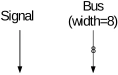
Signals are displayed in block diagrams as arrows, and signal busses are displayed in block diagrams as arrows with a number superimposed on the arrow, which represents the bus width, as shown in Figure 1.

[image:14.612.258.376.437.512.2]

8

Signal

(width=8)

Bus

(15)

Chapter 1

Introduction

With the advent of neural network processing, computer systems have been able to

replace, and in some cases improve upon human operators. One such system would be

auditory processing. Auditory processing is being developed to solve problems such as

voice recognition, speaker recognition, multimedia indexing, SONAR analysis, and many

others [1]. In order to present audio samples to a neural network, the important features

of the sample must first be extracted. Discreet wavelet transform processing combined

with feature extraction techniques have been shown to be effective in this task [2]. The

proposed system incorporates a discreet wavelet transform processor, which employs a

novel hierarchical filtering architecture, as well as a novel data control system for loading

and propagating audio samples and wavelet coefficients, a feature extraction processor,

and a neural network, which was trained with a novel algorithm, to classify audio

samples as belonging to either a voice class or music class. The system was modeled in a

(16)

Part

I Review

of

Literature

Chapter 2

Wavelet

Transform

Theory

Signal analysis has benefited from mathematical tools, such as the Fourier transform and

more recently, wavelet transforms, which manipulates the signal into a more usable form

for analysis. The principal of superposition has been used to approximate functions since

the early 1800’s, when Joseph Fourier discovered that any periodic function could be

represented by superimposing sine and cosine functions. Since Fourier’s transform relies

on the use of non-local periodic functions to approximate target functions, attempting to

represent local non-periodic functions with discontinuities and sharp spikes results in a

less accurate approximation. The wavelet transform is effective in approximating such

functions, as it uses local non-periodic basis functions in its analysis [3].

Another key component of the wavelet transform is its multi-resolution analysis. If

examining a function using a small “window”, small details of that function within that

window would be readily apparent. If examining the same function with a large window,

the gross features of the function would be revealed. The multi-resolution analysis of the

wavelet transform approximates the function in such a way that both the small details are

represented, as well as the gross features, and all scales in between [3].

Wavelet analysis is accomplished by first choosing a representative prototype function,

called the mother wavelet, or analyzing wavelet. The target function is then

approximated by using contracted and dilated versions of the prototype function. The

(17)

analysis, and decreased frequency analysis. The dilated, lower frequency versions of the

prototype result in an increased capacity for frequency analysis, and decreased temporal

analysis. Together, these contracted and dilated prototypes perform an analysis that gives

a complete representation of the target function, both in the time and frequency domains

[3].

2.1

History of Wavelets

Joseph Fourier, the father of Harmonic Analysis, began a field of mathematics, which

eventually lead future mathematicians to Wavelet Analysis. Fourier, in 1807, postulated

that any periodic function f(x) can be expressed as the sum

∑

∞

=

+ +

1

0 ( cos sin )

k

k kx b kx

a

a (1)

of its Fourier series. The coefficients, a0, ak, and bk, are calculated by

∫

= =

= π π π

π π π 2 0 2 0 2 0

0 ( )sin( )

1 , ) cos( ) ( 1 , ) ( 2 1 dx kx x f b dx kx x f a dx x f

a _k _k

For the remainder of the 19th century, researchers investigated the meanings and

applications of Fourier’s frequency analysis, which led those of the early 20th century to

explore the concept of scale analysis. Scale analysis involves constructing a function,

and then scaling and shifting it, and then applying it to a target function to obtain an

approximation. This process is then repeated by shifting and scaling until a complete

(18)

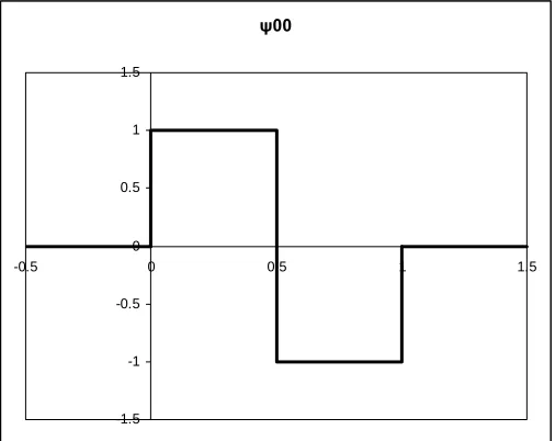
Wavelets were first mentioned in the appendix of Alfred Haar’s thesis in 1909. Haar

showed that any continuous function f(x) on the unit interval [0,1], could be

approximated by a series of step functions. The Haar wavelet is the simplest possible

wavelet which is a step function with the definition

⎪ ⎩ ⎪ ⎨ ⎧ < ≤ − < ≤ = otherwise x x x f 0 , 1 1 , 0 1 )

( 12

2 1

(2)

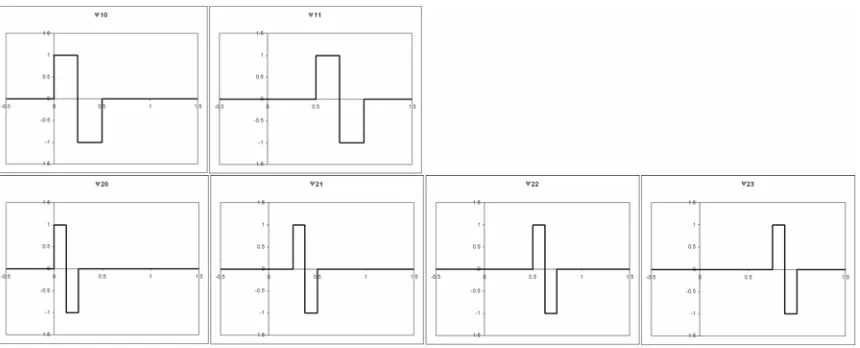
and shown in Figure 2. Figure 3 shows how the Haar mother wavelet ψ00 is dialated by

narrowing its support, and shifted along the unit interval. The individual elements are

linearly independent and can represent step functions of increased thinness.

ψ00 -1.5 -1 -0.5 0 0.5 1 1.5

[image:18.612.180.433.379.580.2]

-0.5 0 0.5 1 1.5

(19)

[image:19.612.93.523.70.244.2]

Figure 3 - Haar Wavelet dilation and shift

The Haar wavelet has compact support, because it disappears beyond a finite interval, but

because it is not continuous, it is also not differentiable, which limits some of this

wavelet’s application [3].

Wavelet research continued since the 1930’s to include an application of Haar’s wavelet

in the study of Brownian motion by Paul Levy, who found it superior to Fourier functions

in studying the small details of the motion. In the latter half of the twentieth century,

Guido Weiss and Ronald R. Coifman analyzed a function space by reducing it to its

“atoms”, and defined assembly rules for these most primitive elements. Jean Morlet and

Alex Grossman [3], whom originally worked windowed Fourier analysis, further

developed wavelet theory by discovering that a wavelet transform could be reversed

losslessly to restore the original function, and that any changes to the wavelet coefficients

resulted in very small changes to the reverse transformed signal. Stephane Mallat [3]

(20)

and orthonormal wavelet bases. He further developed an iterative approach to the

wavelet transform with a filter which employs a pyramid algorithm, laying the foundation

for the Fast Wavelet Transform (FWT), the wavelet correspondent to the Fast Fourier

Transform (FFT). Yves Meyer [3] created the first non-trivial wavelet, which was

continuously differentiable, but lacked compact support. Ingrid Daubechies has the

honor of having created the most elegant wavelet function that has become the

cornerstone of wavelet applications today. The Daubechies families of wavelets are both

continuously differentiable, and have compact support [3,5].

2.2

Fourier Analysis

Fourier’s concept of the superposition of sine and cosine to approximate functions has

had relevant application ranging from the pure mathematical of solving differential

equations to the applied engineering of analyzing communication signals [3].

The Fourier transform’s value is in its ability to allow a periodic function in the time

domain to be analyzed for its frequency content. This is accomplished by first

transforming the time domain function into a function in the frequency domain. The

Fourier coefficients generated in this process directly correspond to the contribution of

the associated sines and cosines at each frequency. The inverse Fourier transform

converts a function from the frequency domain, back into the time domain [3].

The Discrete Fourier Transform (DFT) approximates the Fourier transform of a function

from a finite number of discrete samples, which are representative of the remainder of the

function. The discrete Fourier transform shares many of the symmetry properties of the

(21)

calculation to compute the discrete Fourier transform as the Inverse Discrete Fourier

Transform (IDFT).

DFT: 1 0,..., 1

0 2 − = =

∑

− = − N k e x X N n kn N i n k π (3)

IDFT: 1 1 0,..., 1

0 2 − = =

∑

− = N n e X N x N k kn N i k n π (4)

The Fourier transform does an excellent job of representing periodic continuous functions

with sines and consines. It struggles, however, to represent non periodic or discontinuous

functions. One approach would be to extend the function to attempt to make it periodic,

but one would also need to make the endpoints continuous. For this reason, the

Windowed Fourier Transform (WFT) was created to address this problem. The WFT

chops up a signal into time slices, and then analyze the frequency content of the function

bounded by its window. The endpoints of the function at the window boundaries could

still present a problem to the Fourier transform however, so a weighting system is used to

bias the endpoints toward a value of zero. The WFT also has the added benefit of

localizing the frequency analysis in time [3].

In the case of using the discrete Fourier transform to approximate the Fourier integral of

the sampled function, the DFT equation (3) requires a calculation of the order O(n2) for a

function of n samples. The problem quickly grows in complexity as the sample size

increases. For this reason, it is important to discuss the valuable contributions of J. W.

Cooley and J. W. Tukey in 1965, who proposed a solution to the DFT which only

(22)

recursively dividing the calculation from a DFT of size N = N1N2into separate DFT

calculations each of size N1 and N2 respectively. Their work resulted in the so called fast

Fourier transform (FFT) [3].

2.3

Comparison of Wavelet Analysis to Fourier Analysis

The wavelet transform shares many similarities to the Fourier transform. For example

both the Discreet Wavelet Transform (DWT) and the Fast Fourier Transform (FFT) are

linear operations which generate log2 n vectors of varying lengths, which when combined

form a vector of 2n total length. The similarities also extend to the matrices involved in

these calculations. The inverse transforms for both the DWT and FFT use the transpose

of the matrix from the forward transform. Therefore, each transform can be considered a

rotation of function space to a different domain. Both transforms are also dependent on

the use of basis functions; the FFT uses sine and cosine basis functions, and the DWT

uses a more complicated basis function called a wavelet, a mother wavelet, or an

analyzing wavelet. These basis functions are localized in frequency, both for the FFT

and the DWT, which makes them useful for such calculations as power spectra [3].

The dissimilarities between the wavelet transform and the Fourier transform give the

wavelet transform advantages in many types of time series analysis. The most significant

dissimilarity is that wavelet functions are localized in space, whereas the sines and

cosines of the Fourier transform are not. Wavelet function’s time localization combined

with its frequency localization give functions transformed into the wavelet domain a

sparse nature, which makes them particularly useful for feature detection, removing noise

(23)

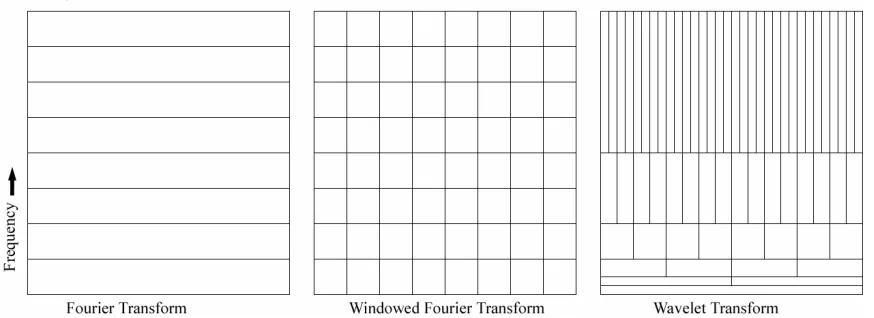
One way to visualize the difference between the time-frequency resolution of the Fourier

transform and the wavelet transform is to examine the basis function coverage of the

time-frequency plane. In Figure 4, the time-frequency coverage is compared between the

[image:23.612.89.526.204.363.2]

Fourier transform, the windowed Fourier transform, and the wavelet transform.

Figure 4 - Comparison of Time and

Frequency Resolution

It can easily be seen from Figure 4, that the Fourier transform has no time resolution, and

only frequency resolution. This is because the sine and cosine basis functions are infinite

in length, and only change in frequency. The windowed Fourier transform shows the

same time resolution at all frequencies, because the size of the window in the WFT is the

same at all frequencies, and truncates the sines and cosines [3].

With the wavelet transform, the time resolution changes at each frequency analyzed. For

analysis of small discontinuities, it would be beneficial to have some very short basis

function, but for detailed frequency analysis, very long basis functions would be required.

(24)

functions as well as very long low frequency basis functions, as shown in Figure 4. An

important quality of the wavelet transform is that there is an infinite set of different basis

functions to choose from, where as Fourier transforms utilize only the sine and cosine

basis functions. Wavelet analysis provides direct access to information that might

otherwise be obscured by other time-series analysis methods such as the Fourier

transform [3].

2.4

Wavelets in Audio Processing

In the case of digital audio processing, a discreet transform can be used in the analysis of

a digital signal. Discreet Wavelet Transform (DWT) analysis is of greater benefit to audio

processing than Discreet Fourier Transform (DFT) analysis, because DWT analysis is a

multi-resolution representation that includes both time and frequency localization,

whereas DFT analysis only provides frequency localization [7]. Features generated, from

time and frequency information, are of greater value to audio analysis than are features

generated from frequency information alone, because this closely approximates human

auditory processing [8].

A wavelet is a mathematical function, which, when applied to a signal, generates a

multi-resolution time-frequency representation of that signal. This is similar to a sub-band

encoding, in which each successive sub-band has incrementally more time representation,

and incrementally less frequency representation. The time-frequency components are

generated by sets of scaling functions and wavelet functions, which are associated with

low-pass and high-pass filters, respectively. The time domain signal is successively

(25)

down-sampled. After each stage of low- and high-pass filtering, the resulting half bands

contain the same number of samples as the input, but half the frequency. According to

the Nyquist Criterion, half of the resulting samples can be discarded without loss of

information. The down-sampled outputs of the high-pass filter of each stage become

wavelet detail coefficients, and the down-sampled outputs of the low-pass filter are again

processed by the low- and high-pass filters of the next stage, with the final stage outputs

of the low-pass filter being the wavelet approximation coefficients. The combination of

the approximation coefficients and the detail coefficients from each stage becomes the

DWT coefficients, or wavelet coefficients [9, 10].

Since the low-pass filter effectively removes half of the frequencies, the resulting signal

has twice the frequency resolution of the input signal. However, since half of the

resulting samples are discarded due to down-sampling, the time resolution is halved.

Therefore, the successive filtering and down-sampling produces coefficients with a

greater frequency resolution, and a lesser time resolution after each stage of the process.

Therefore, the generated detail coefficients of each stage have increased frequency

resolution, but reduced time resolution. Unlike DFT, the time localization of the signal is

maintained as well as the frequency localization, however it localized within a resolution.

Signal analysis often requires a multi-resolution approach, which makes this scheme an

(26)

Chapter 3

Feature

Extraction

Theory

3.1

Time Series Similarity

The problem of data comparison is often fairly trivial for most data domains. One must

merely determine the similarity or equality of one or more attributes for a datum to

compare against another in the same given domain. This procedure is not inherently

extensible to comparing one time series to another, because there are no inherent

attributes of a time series with which to compare [12]. The problem of generating

attributes for a time series with which to compare has been a topic of recent interest, and

several approaches have been proposed. This chapter covers two such approaches, the

latter of which was implemented in this thesis. The Struzik and Siebes approach [13] to

generating attributes for a time series results in features that can be directly compared via

a quadratic distance measure. The Pittner and Kamarthi approach [2] to generating

attributes for a time series results in features that are designed to be directly processed by

a neural network.

3.2

The Struzik and Siebes Approach

When comparing time series, one would want to choose a comparison that ignores bias,

both constant and linear, and also ignores scale, both in time and amplitude. Subjective,

qualitative judgments of similarity (by humans) are based on non-stationary behavior,

rapid transients that indicate beginnings of trends, large fluctuations, and rare events.

Whereas a statistical estimation of a time series would be thwarted by such fluctuations,

these statistical deviations can be measured and transformed into features for time series

(27)

Struzik and Siebes found that by applying the wavelet transform to the time series the

local behavior of the function is revealed, as well as the above mentioned biases are

suppressed. They also found the wavelet transform to be excellent at characterizing

non-stationarities, as well as to reveal the hierarchy of singular features including their scale

free behavior. Using Mallat’s [14] representation of the wavelet transform, the Wavelet

Transform Modulus Maxima (WTMM), they could characterize local singular behavior

of time series. The WTMM can also be used for the evaluation of the Hölder exponent of

the singularity:

, )

,

( ₀ ( )

)

(n _f _s _x _sh x0

W ≈ (5)

if h(x0) < n + 1, where n indicates the number of vanishing moments of the wavelet. The

Hölder exponent can be used as a representation of the roughness or smoothness of the

time series, where larger values of the Hölder exponent relate to smoother, more regular

time series [13].

Struzik and Siebes’ approach to generating attributes for a time series involves including

a certain number of predefined features. These features are obtained by taking the

predefined number of strongest maxima, and then tracing them below the representation

scale from which they appear. This method allows for better localization of singularities

in the time domain, as well as to gain a more stable estimation of the Hölder exponent.

For a given maxima, the datum recorded has the following attributes: the x-coordinate xi,

the Hölder exponent h(xi), and the corresponding sign of the wavelet transform Wf(xi).

These features can then be compared by means of a quadratic distance measure, with

(28)

), (

1 ) ,

( _x _x2 _h _h2

s x h f f

dist = − Δ + Δ (6)

where Δ_x =x−x_i and Δ_h =h−h_i and xi,hi belong to s, the representation of the time

series [13].

3.3

The Pittner and Kamarthi approach

The data provided by the wavelet decomposition process, though multi-resolution and

time- and frequency-localized, is not of an acceptable form for neural network

processing. The wavelet coefficient data set is overly large, and includes data that could

be not meaningful or could be misleading to the training or classifying process of neural

networks. A feature extractor processor, to generate meaningful features from the

wavelet coefficients, is required. The feature extraction process described by Stefan

Pittner and Sagar V. Kamarthi [2] was chosen for this thesis.

The feature extraction process requires initial setup steps that involve processing a

training set of data. This training set is the same data set that will be used to train the

neural network. The use of the training set allows the feature extraction process to be

customized for the data space of interest. The feature extraction process depends on the

use of clusters to identify groups of wavelet coefficients. The determination of the

number of clusters and the size of each cluster is accomplished by the following

procedure. First, the coefficients are placed in a matrix, B, such that each row vector

contains all of the detail coefficients for a given level of decomposition, and the last row

vector contains the approximation coefficient. All empty spaces in the matrix are filled

(29)

an array of matrices, BK, where K is the length of the training set. Let I be the matrix of

the same size as B but containing only 1’s as its elements. Let R be the operation that

reduces a matrix by its last row. A matrix, G, is calculated by the following equation.

⎟ ⎟ ⎠ ⎞ ⎜ ⎜ ⎝ ⎛ ⋅ ⎟⎟ ⎠ ⎞ ⎜⎜ ⎝ ⎛ ⎟ ⎠ ⎞ ⎜ ⎝ ⎛ − ⎟⎟ ⎠ ⎞ ⎜⎜ ⎝ ⎛ ⎟ ⎠ ⎞ ⎜ ⎝ ⎛ = =

∑

= = = I B R B B R g G K k k K k k K k k ij 1 1 1 1 : ) ( μ σ

. (7)

By applying a threshold of the form T := 2

(

lnL−lnγ

)

with _γ _≥_e2_{to the elements of the}

matrix G, with L being the number of computed detail coefficients, the binary matrix,

(

)

(

g T

)

G_b := Θ _ij − , (8)

is obtained, where the Heavyside function Θ

( )

x =1 for x≥0 and Θ

( )

x =0 for x<0 [7].

The binary matrix, Gb, contains 1’s at the center of the proposed clusters. If a row vector

of Gb contains no 1’s, the entire row vector is treated as a cluster. This ensures that

clusters do not overlap across different scales.

Extracting the features of the wavelet coefficients involves using the clusters that were

generated. For each cluster, U, the feature, u, is calculated by taking the square root of

the sum of the squares of each coefficient, v, in the cluster, also known as the Euclidean

norm [2].

∑

∈ = = i U v i

i r v

u 2

2

(30)

Chapter 4

Neural

Network

Theory

4.1

Perceptron Theory

Neural networks can be applied to solve classification problems by means of a learning

process. Using the learning process, the solution to the classification problem can be

found without the need for complex, often slow and inaccurate, algorithms. There are

varieties of different types of neural networks that have been proposed by researchers.

One of which, is the multi-layer perceptron, which has its basis in neural biology [15].

The multi-layer perceptron has been found to be the classic solution in the task of

classifying signal based problems [16, 17].

The basic building block of the multi-layer perceptron is the artificial neuron, also known

as the perceptron. The McCulloch-Pitts model of a neuron [15] is represented by

synapses, an adder, and an activation function. The synapses are the inputs to the neuron,

each with its own weight in order to adjust the strength of the input. The adder

component combines the inputs of the neuron, and multiplies each by its respective

weight. This weighted sum is called the activation potential. The activation function

then applies a “squashing function” to the activation potential. This limits the

permissible amplitude range of the output signal [15]. For linearly separable classes, a

simple threshold function would suffice for the activation function, such as

⎩ ⎨ ⎧

< −

≥ =

0 ,

1 0 ,

1 ) (

x x x

(31)

The model of a perceptron, considered for this thesis, is based on the McCulloch-Pitts

model of a neuron. The goal of the perceptron is to correctly classify a set of inputs. In

the simplest form of the perceptron, there are two decision regions separated by a

hyper-plane. Therefore, these classes must be linearly separable. The perceptron is trained with

a known training set, which must be limited to two linearly separable classes. The

perceptron converges using an error back propagation learning algorithm [15].

4.2

Multi-Layer Perceptron Neural Network Theory

The model of the multi-layer perceptron, considered for this thesis, is based on the single

perceptron. The goal of the multi-layer perceptron is to correctly classify a set of inputs

within an input space that is defined by more than two decision regions, and is therefore

non-linear.

The activation function must be a non-linear function, in order that the perceptron can

classify patterns that are not linearly separable. For non-linearly separable classes, a

sigmoid function is traditionally chosen because of its simple derivative. Examples of

sigmoid functions include the special case of the logistic function, where

x

e

x ₋

+ =

1 1 ) (

φ , (11)

and the hyperbolic tangent, where

) tanh( )

(x = x

φ [18]. (12)

This thesis employs the following theoretical model of the neuron. The neuron function

(32)

∑

=

⋅ = m

j

j kj

k w x

v

0 ₍₁₃₎

The activation function for each neuron is defined to be

(

v_k(n)

)

a tanh

(

b v_k(n)

)

k = ⋅ ⋅

φ _. ₍₁₄₎

Values for a are chosen to allow for adequate buffering between the desired response and

the actual response. Values for b are chosen to allow for a larger range of vk values, in

order to avoid railing the actual response.

The number of layers and the number of neurons in each layer determine the number of

decision regions that a multi-layer perceptron can define. A typical multi-layer

perceptron consists of an output layer, and one or more hidden layers, one of which is

also known as the input layer. The multi-layer perceptron is first trained with a known

training set. This is accomplished by applying the known input to the input layer, and

then forward propagating the results through the other layers. During this phase, the

weights remain constant. The results from the output layer are then collected, and

compared to the desired response, which is determined from the known input. An error

signal is calculated from the difference of the actual response and the desired response.

This error signal is then back propagated through the neural network, against the

direction of the synaptic connections. The multi-layer perceptron converges using a

back-propagation error-correction learning algorithm [15].

After each training iteration, the weights in the neural network are modified according to

(33)

( )

n y

( )

n

w_ji = ⋅ _j⋅ _i

Δ η δ , (15)

where η is the learning rate, and yi is the neuron output value.

If j is in the output layer,

( )

(

( )

)

(

a y

( )

n

)

(

a y

( )

n

)

a b n y n d

n _j _j _j _j

j = − ⋅ ⋅ − +

δ , (16)

or if j is in a hidden layer,

( )

= ⋅

(

−

( )

)

(

+

( )

)

⋅

∑

( )

⋅

( )

k kj k j j

j a y n a y n n w n

a b

n δ

δ , (17)

where dj is the desired response, and a and b are the scaling values from the neuron

activation function. Training continues until the weights of the neural network produce

outputs that converge. Convergence is defined by an average error signal, εav reaching a

threshold.

( )

n d

( )

n y

( )

n

e_j = _j − _j (18)

( )

∑

( )

∈ ⋅ = c j j n e n 2 2 1

ε , (19)

where c is the set of all neurons in the output layer.

( )

∑

= ⋅ = N n av n N 1 1 _ε

(34)

Chapter 5

Wavelet Neural Network Theory

5.1

Overview of Wavelet Neural Networks

Applications of Wavelet Neural Networks (WNN) are nearly as varied as their possible

configurations. Two popular applications of WNNs are their use as function

approximators, and as signal classifiers, the latter of which is the focus of this thesis. In

the domain of time series analysis, Wavelet Neural Networks improve upon the classic

Artificial Neural Network (ANN). ANNs have limited ability to characterize local

features of a time series, which are generally critical to accurately classifying or modeling

the series. Since these features are often localized in time and/or frequency, employing

wavelets enables the Neural Network to take advantage of the multi-resolution analysis

offered by wavelets to focus the network on these local features [19]. Generally speaking,

a wavelet function is used to condition the inputs to the neural network, such that only

vital information about the signal is processed by the network. When designing a

Wavelet Neural Network, the possible configurations of wavelet functions, neural

network architectures, and their integrations, are nearly limitless.

5.2

Wavelet Neural Networks as Function Approximators

The use of Wavelet Neural Networks as function approximators lends to applications

involving process modeling, non-linear function approximation, non-parametric

estimation, control tasks, time series forcasting, and many others [19]. As opposed to

classical ANNs which use sigmoidal-based activation functions, WNNs of this type

(35)

function for the hidden layer neurons, and a linear output layer which represents the

weighted sum of the hidden layer.

Each neuron in the hidden layer represents a wavelet coefficient, such that its

corresponding IDWT is localized in time and frequency with a given dilation and

translation [20]. Since the wavelet transform results in a sparse representation, not all of

the wavelet coefficients are necessary for an accurate reconstruction of the original signal

[21]. In fact, the inclusion of all of the coefficients would likely cause over training of

the neural network, and result in poor convergence. For this reason, wavelet coefficients

that do not contribute to the local features of the signal are identified during the iterative

training of the WNN, and their corresponding neurons are pruned from the network [22].

As an application of this technology, Geva discusses a modification to this architecture

called ScaleNet [23]. ScaleNet is a multiscale Neural Network architecture for time

series prediction. For history based prediction to succeed, information must be present in

the history of the time series that indicates the future of the time series. Geva’s approach

to this problem results in a three stage architecture consisting of a wavelet analysis of the

history of the time series, which feeds into several independent feed-forward neural

networks, each responsible for one scale of the wavelet decomposition. The results of

each neural network, wavelet coefficients of the predicted time series increment, are then

propagated to a final stage perceptron which combines each weighted contribution to the

(36)

5.3

Wavelet Neural Networks as Classifiers

The use of Wavelet Neural Networks as classifiers lends to applications involving

machine failure mode analysis, and auditory processing tasks, including voice

recognition, speaker recognition, multimedia indexing, SONAR analysis, and many

others. WNNs of this type are typically found in one of two main configurations. One of

these configurations involves a neural network which uses wavelets as activation

functions, such that each neuron implements the DWT at a different dilation and

translation.

Wang, Yu, and Lee [24] discuss the application and implementation of a WNN of this

configuration. The application of their WNN involves machine failure mode analysis,

such that sensors on the machine provide the WNN a steady time series of information.

An analysis of the time series can reveal the health of the machine, from normal, to

degraded, to failure. The neural network was trained with widowed samples of each of

these states, resulting in a WNN capable of indicating to an operator when the machine is

in the degraded state, before it fails [24].

The other configuration of WNNs used for classification, such as the one modeled in this

thesis, involves a wavelet preprocessor, feature extractor, and a classic sigmoidal-based

ANN to classify the time series. A window of the time series is converted to wavelet

coefficients by the wavelet preprocessor, and then features are generated from the

wavelet coefficients, which are then fed to the input (hidden) layer of the ANN. This

configuration of WNN can be trained to classify the windowed time series through

(37)

Part II

Design Implementation of a Wavelet Neural

Network

Chapter 6

Design Implementation of a Wavelet Transform

The Haar wavelet transform was chosen as the DWT for this thesis because it lends well

to a digital design, and it is the simplest of the wavelet transforms, yet has been proven

effective in signal analysis. The Haar transform can be implemented rather easily, it

requires minimal intermediate storage, and it’s computation is bounded by order O(n),

which allows for a pipelined digital design [7]. Conceptually, the Haar wavelet transform

is a recursive filtering, beginning first with the original sample vector, which is processed

by both a low-pass and a high-pass filter. The output of the high-pass filter is collected to

the result vector as detail coefficients, and the output of the low-pass filter is successively

filtered as previously described. This repeats until each filter generates only one

coefficient. The output of the final low-pass filter is the approximation coefficient. This

(38)

[image:38.612.97.505.71.472.2]

Figure 5 - Haar DWT Processing [9]

The low-pass filter produces outputs that are the sum of adjacent inputs divided by two,

and the high-pass filter produces outputs that are the difference of adjacent inputs divided

by two. The outputs of each filter are of the same number as the inputs, but have half the

frequency band. Therefore, half of the outputs can be discarded, according to the Nyquist

Criterion. Thus, the transform process can be performed in log2(n). stages, where n is the

(39)

approximation coefficient. If the process were performed in reverse, the original signal

could be reconstructed; therefore, there is no loss of information in this procedure [9]. A

frame size of 256 input samples was chosen for this thesis, which has been determined to

be an effective, yet minimal size [16].

6.1

Software Simulation

The design of the wavelet transform processor for the software simulation was fairly

straightforward. The Wavelet class accepts a 256-entry array of 16-bit audio samples as

inputs, and generates a 256-entry array of 4-bit wavelet coefficients. The Wavelet class

consists of a process function which calls a filter function on the input samples and then

successively on the resulting filtered outputs. The filter function in turn calls both a high-

and a low-pass function. For each of the adjacent pairs of the input set, the high-pass

function computes the difference of the pair, and divides the difference by two. For each

of the adjacent pairs of the input set, the low-pass function computes the sum of the pair,

and divides the sum by two. The outputs of the high-pass filter, the detail coefficients,

are collected in a result array, and the outputs of the low-pass filter are propagated to the

filter function of the next processing stage. This procedure continues until the high- and

low-pass filters produce a single output. The final output of the high-pass filter is stored

in second position of the result array, and the final output of the low-pass filter, the

approximation coefficient, is stored in the first position of the result array. Following the

filtering operations, the coefficients are converted to 4-bit values by means of shifting

(40)

6.2

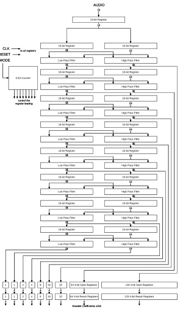
Digital Design Implementation

A novel approach was taken in the design of the wavelet transform processor for this

thesis. The wavelet transform processor was designed to accept uncompressed digital

audio, sampled at 11.025 kHz at 16 bits per sample. The digital audio is processed in

blocks of 256 samples or approximately 23 milliseconds. This requires log2(256) = 8

levels of filters to transform the audio data into wavelet coefficients. Instead of designing

an expansive tree of filters and intermediate registers to simultaneously perform the

transform operation on the entire block of 256 samples, a novel approach was used in the

design to pipeline the samples through 8 levels of low- and high-pass filters and

intermediate capture registers. An intricate control system was designed to control the

loading and propagating of the data at the intermediate capture registers and the result

registers. Due to synchronization issues, the process takes more than 256 cycles to

complete. Therefore, an additional pipeline stage of temporary save-registers were used

to prevent the overwriting of the results by the processing of the next block of samples.

The wavelet transform processor’s outputs are 256 4-bit wavelet coefficients. A block

diagram of this system is shown in Figure 6. A block diagram of the high and low pass

(41)

AUDIO

CLK RESET MODE

16-bit Register 16-bit Register

16 16

16 Low Pass Filter High Pass Filter

16

16 16

16

16 16

16

16 16

16

16 16

16

16 16

16

16 16

16

16 16

Low Pass Filter High Pass Filter

128 4-bit Save Registers 64 4-bit Save Registers

32 16 8 4 2 1 1 16 16 8-bit Counter to all registers

control the register loading

4 4 4 4 4 4 4 4 4

16-bit Register 16

128 4-bit Result Registers 64 4-bit Result Registers

32 16 8 4 2 1 1

Wavelet Coefficients x256

4 4 4 4 4 4 4 4 4

16

AUDIO

CLK RESET MODE

16 16

16

16 16

16

16 16

16

16 16

16

16 16

16

16 16

16

16 16

16

16 16

4 4 4 4 4 4 4 4 4

16-bit Register 16

32 16 8 4 2 1 1

4 4 4 4 4 4 4 4 4

16

AUDIO

CLK RESET MODE

16 16

16

16 16

16

16 16

16

16 16

16

16 16

16

16 16

16

16 16

16

16 16

4 4 4 4 4 4 4 4 4

16-bit Register 16

32 16 8 4 2 1 1

4 4 4 4 4 4 4 4 4

[image:41.612.130.485.66.684.2]

16

(42)

Carry Look-Ahead Adder

16 16

Low Pass Unit

0 Ci

16

High Pass Unit

1 Ci 16

0 _Ci 1 16

16

bit 15

bit 15 bits 15-1 Mux

0 _Ci 1 16

16

bit 15

[image:42.612.92.524.68.343.2]

bit 15 bits 15-1 Mux

(43)

Chapter 7

Design Implementation of a Feature

Extraction

The design of the feature extractor processor closely follows the feature extraction

process described previously. In a software development environment, the training set of

audio samples was transformed by the wavelet process into wavelet coefficients. The

feature cluster analyzer software, as described above, then processed these wavelet

coefficients. This resulted in discovering 34 clusters for the data space considered in this

thesis.

7.1

Software Simulation

The feature cluster analyzer software was designed to take the training set of wavelet

coefficients, and calculate the boundaries of the feature clusters. This was accomplished

by means of software to calculate the G matrix, and a spreadsheet to calculate the Gb

matrix.

The software to calculate the G matrix, read files containing the stored voice and music

wavelet coefficients from the training set, and constructed a B matrix for each set of 256

coefficients. These B matrices were placed in an array Bk, which was then used to

calculate the G matrix, in a process, described in equation (7). The G matrix was then

(44)

The spreadsheet used to calculate the Gb matrix was created from the stored G matrix file.

The threshold T was then subtracted from each element of the G matrix. The threshold T

was calculated to be 2.6613, by using the equation, T:= 2

(

lnL−lnγ

)

, where L is the

number of detail coefficients, which is 255, and γ is greater than or equal to e2_{, which was}

chosen to be e2. The Heavyside function was then applied to each element of the

intermediary matrix, as described in equation (8), which resulted in the Gb matrix. For

illustrative purposes, the resulting Gb matrix is depicted graphically in Figure 8. Black

squares represent 1’s in the binary matrix, and white squares represent 0’s. Gray squares

represent areas of the matrix that have no corresponding wavelet coefficient. The bottom

left square represents the approximation coefficient, and the remaining non-gray squares

represent the eight levels of detail coefficients.

Figure 8 -

G

b

Matrix for Feature Cluster Detection

The feature clusters were determined by using each “1” in the matrix as the approximate

center of the cluster. If a matrix row had no 1’s, the entire row was designated as a

cluster. This ensured that clusters did not overlap across different scales. The resulting

(45)

{d1(0),…,d1(5)} {d1(6),…,d1(9)} {d1(10),..,d1(15)} {d1(16),…,d1(24)} {d1(25),…,d1(35)} {d1(36),…,d1(44)} {d1(45),…,d1(49)} {d1(50),…,d1(57)} {d1(58),…,d1(74)} {d1(75),…,d1(94)} {d1(95),…,d1(108)} {d1(109),…,d1(127)} {d2(0),…,d2(8)} {d2(9),…,d2(15)} {d2(16),…,d2(19)} {d2(20),…,d2(22)} {d2(23),…,d2(33)} {d2(34),…,d2(44)} {d2(45),d2(46)} {d2(47),…,d2(52)} {d2(53),…,d2(58)} {d2(59),…,d2(63)} {d3(0),…,d3(12)} {d3(13),…,d3(16)} {d3(17),…,d3(25)} {d3(26),…,d3(31)} {d4(0),…,d4(9)} {d4(10),…,d4(13)} {d4(14),d4(15)}

{d5(0),…,d5(7)}

{d6(0),...,d6(3)}

{d7(0),d7(1)}

{d8(0)}

[image:45.612.69.718.88.226.2]

{a8(0)}

(46)

The design of the feature extractor processor for the software simulation was

straightforward. The FeatureExtractor class accepts a 256-entry array of 4-bit wavelet

coefficients as inputs, and generates a 34-entry array of 4-bit wavelet features. The

FeatureExtractor class consists of a process function that computes the square root of the

sum of the squares of each wavelet coefficient within the predefined boundaries of each

feature cluster, as described in equation (9).

7.2

Digital Design Implementation

The digital design of the feature extractor processor consists of a feature extractor

module, which contains 34 cluster processors. Each cluster processor performs the

operations described in equation (9). The feature extractor module accepts wavelet

coefficients as inputs, which it allocates to the cluster processors according to the cluster

boundaries. The feature extractor processor outputs 34 4-bit wavelet features. Block

diagrams of this system are shown in Figures 9 and 10.

CLK RESET

MODE

Wavelet Coefficients x256 4

Wavelet Features x34 ₄ ₄ Feature Cluster

Unit

Feature Cluster Unit

Feature Cluster Unit ... 34 Feature

Cluster Units ...

4 4

20 inputs 20 inputs 20 inputs 20 inputs 20 inputs

4 4 4 4 4

(47)

CLK

RESET

MODE 4 4 4 4 4 4 ... 4 4 4 4 4 4 4 4

4x4 multiplier 5

8-bit Register 8-bit Register 8

8 8 0 Ci

8-bit Register Done?

5

8

8-bit Square

Root 8

4 Wavelet Feature 20 Input Mux

5-bit Counter

4

Bit 3

Carry Look-Ahead Adder 0 _Ci=1

Mux

4

4 4

4

8

(48)

Chapter 8

Design Implementation of a Neural Network

The neural network considered for this thesis was a 2-layer multi-layer perceptron

consisting of 34 input neurons, and 2 output neurons. The 34 wavelet-features were fully

connected to the 34 input neurons, which were in turn, fully connected to the output

neurons. Each output neuron corresponds to each of the two result classes, voice and

music.

8.1

Software Simulation

The design of the neural network processor for the software simulation consists of a

NeuralNetwork class and a Neuron class. The NeuralNetwork class accepts a 34-entry

array of 4-bit wavelet features as inputs, and generates a result classification of “voice”,

“music”, or “other”. The NeuralNetwork class primarily consists of 34 input Neuron

objects, 2 output Neuron objects, a training function, and a testing function. The Neuron

class primarily consists of an input array, a weights array, an Activate function, and an

output. The Neuron Activate function performs the operations in Equations (13) and (14)

on the input array to generate the output.

The NeuralNetwork training function is called to determine the best values of the weights

in each of the neurons for a given training data set. The neural network parameters were

determined experimentally beginning with typical values [15]. Given the 8-bit weight

limitation imposed on the system, a novel approach was taken in the design of the

training algorithm. The training algorithm performs the operations in Equations (15)

(49)

calculating the desired response. The training algorithm then updates the weights in each

neuron according to the difference between the response from the neurons, and the

desired response. If during the training process, the weights of a neuron exceed the

bounds of an 8-bit value (-128 to 127) before convergence is reached, all of the weights

for that neuron, and for each neuron in its layer are reduced by half. By applying this

reduction across the entire layer, the relative strengths of each weight for each neuron is

maintained, while allowing for further fine tuning of the weights, resulting in eventual

convergence. This reduction by half algorithm generated far better results than when the

weights were allowed to grow unbounded and then scaled to 8-bit resolution after

convergence. After training, the weights from each neuron can be downloaded to a file.

The NeuralNetwork testing function classifies inputs once each neuron’s weights have

been established by training. The weights can also be uploaded from a file. The testing

function is called with a test data set of wavelet features. The test data set is processed by

the input neurons, whose results are propagated to the output neurons. The results of the

output neurons determine the final classification for the input set. If the first output

neuron has the largest output, then the classification is “voice”. If the second output

neuron has the largest output, then the classification is “music”. If both output neurons

have an output of zero, then the classification is “other”.

8.2

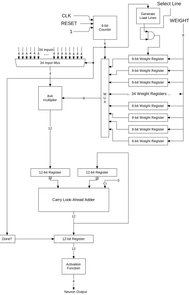
Digital Design Implementation

The digital design of the neural network was inspired by the design in [25]. The weights

(50)

hardware in the design. The training was instead performed in a software simulation

model. To restrict the hardware design to a reasonable size, the neural network data

paths were limited to 4-bit wide busses, and the weights were limited to 8-bit values. The

neural network processor consists of a main neural network module, which contains 34

input neuron modules, 2 output neuron modules, synchronization hardware to ensure

proper data flow through the model, and a result generator module. The result generator

observes the outputs of the output neurons, and generates VALID, VOICE, MUSIC, and

OTHER signals. If the first output neuron’s output is greater than or equal to the

second’s, than the result is “voice”. If the second output neuron’s output is greater than

the first’s, the result is “music”. If both output neurons’ outputs are equal to zero, then

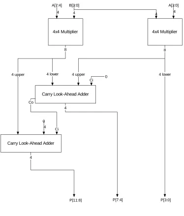
the result is “other”. The input and output neuron modules were similar in design. The

neuron modules contain 8-bit registers to store weights, muxes to select input and weight

combinations, and an 8x4 bit multiplier with an accumulator to implement the activation

potential calculation. The input and output neurons implement individual activation

functions, which are look-up based comparators. A block diagram of this system is

shown in Figures 11 and 12. A block diagram of the 8x4-bit multiplier is shown in

(51)

WEIGHTS

CLK

VALID VOICE MUSIC OTHER RESET

MODE

Wavelet Features x34

Neuron Neuron Neuron Neuron Neuron

Neuron

Neuron Neuron

... 34 Neurons ...

34 Inputs 34 Inputs 34 Inputs 34 Inputs 34 Inputs 34 Inputs

34 Inputs 34 Inputs

8

Determine Result

4 4

To all inputs of input layer neurons

4 4 4 4 4 4

To inputs of ouput layer neurons To inputs of ouput layer neurons

CLK RESET

MODE

6-bit Counter

Generate Select Lines 6

(52)

WEIGHTS CLK

RESET

1

8-bit Weight Register

8-bit Weight Register 8-bit Weight Register 8-bit Weight Register

8 6-bit Counter Generate Load Lines M U X 6 ...

4 4 4 4 4 4 4 4 4 4 4 4 4 4 34 Input Mux

34 Inputs

8x4 multiplier

12-bit Register 12

12 0 Ci 12-bit Register 12 4 8 Done? 12 Activation Function 4 Neuron Output Select Line

... 34 Weight Registers ...

8-bit Weight Register

[image:52.612.111.501.70.678.2]

12-bit Register 12

(53)

0 Ci

Ci

4x4 Multiplier

B[3:0] A[3:0]

4 ₄ 4

A[7:4]

4

Co

0

8 8

4 upper 4 lower 4 upper 4 lower

4

[image:53.612.94.468.66.505.2]

P[11:8] P[7:4] P[3:0]

(54)

Chapter 9

Design Implementation of a Wavelet Neural

Network

Wavelet Neural Networks are essentially neural structures with wavelet filters applied to

extract features of the input set in the time-frequency domain. Since wavelet filters and

neural networks can each take many forms, the combinations and configurations of

wavelet neural networks are practically unlimited. The domain of the problem of

consideration is the classification of digital audio into voice and music classes.

Therefore, a discreet Haar transform with a feature extraction mechanism was combined

with a multi-layer perceptron neural network to form a wavelet neural network.

The wavelet neural network considered for this thesis was a discreet Haar wavelet

processor with a feature extractor processor combined with a 2-layer multi-layer

perceptron consisting of 34 input neurons, and 2 output neurons. The 256 samples of

16-bit digital audio were first applied to the wavelet processor and thereby converted to 256

4-bit wavelet coefficients. The wavelet coefficients were then applied to the feature

extractor processor, resulting in 34 wavelet-features. These wavelet-features were fully

connected to the 34 input neurons, which were in turn, fully connected to the output

neurons. Each output neuron corresponds to each of the two result classes, voice and

(55)

9.1

Software Simulation

The design of the wavelet neural network for the software simulation was

straightforward. The software consisted of a Wavelet ob

An auditory classifier employing a wavelet neural network implemented in a digital design

Rochester Institute of Technology

RIT Scholar Works

AN AUDITORY CLASSIFIER

RELEASE PERMISSION FORM

Rochester Institute of Technology

Abstract

Acknowledgements

Contents

Abstract... iii

Chapter 3 Feature Extraction Theory... 12

Part II Design Implementation of a Wavelet Neural Network... 23

Chapter 10 Simulation Results Comparison between Ideal Software and Digital Design Implementation... 46

List of Figures

List of Tables

SONAR

Terms

Actel ProASICPlus

Digital Signal

Nyquist Criterion

Wavelet Transform

Conventions

Class Naming

Diagrams

Block Diagrams

Signal

I Review

History of Wavelets

Figure 3 - Haar Wavelet dilation and shift

Fourier Analysis

Comparison of Wavelet Analysis to Fourier Analysis

Figure 4 - Comparison of Time and

Wavelets in Audio Processing

Chapter 3

The Struzik and Siebes Approach

The Pittner and Kamarthi approach

Chapter 4

Multi-Layer Perceptron Neural Network Theory

Chapter 5

Wavelet Neural Networks as Function Approximators

Wavelet Neural Networks as Classifiers

Part II

Figure 5 - Haar DWT Processing [9]

Software Simulation

Digital Design Implementation

AUDIO

AUDIO

AUDIO

Chapter 7

Software Simulation

Figure 8 -

Digital Design Implementation

CLK RESET

Chapter 8

Software Simulation

Digital Design Implementation

WEIGHTS

WEIGHTS CLK

Chapter 9

Software Simulation